Magnetic black universes and wormholes
with a phantom scalar

S.V. Bolokhov^a,1, K.A. Bronnikov,^a,b,2 and M.V. Skvortsova^a,b,3

^a

Institute of Gravitation and Cosmology, PFUR, Miklukho-Maklaya St. 6, Moscow 117198, Russia

^b

Center of Gravitation and Fundamental Metrology, VNIIMS, Ozyornaya St. 46, Moscow 119361, Russia

We construct explicit examples of globally regular static, spherically symmetric solutions in general relativity with scalar and electromagnetic fields which describe traversable wormholes (with flat and AdS asymptotics) and regular black holes, in particular, black universes. A black universe is a nonsingular black hole where, beyond the horizon, instead of a singularity, there is an expanding, asymptotically isotropic universe. The scalar field in these solutions is phantom (i.e., its kinetic energy is negative), minimally coupled to gravity and has a nonzero self-interaction potential. The configurations obtained are quite diverse and contain different numbers of Killing horizons, from zero to four. This substantially widened the list of known structures of regular BH configurations. Such models can be of interest both as descriptions of local objects (black holes and wormholes) and as a basis for building nonsingular cosmological scenarios.

PACS numbers: 04.20.-q, 04.20.Jb, 04.40.-b, 04.70.Bw, 98.80.Jk
UDK: 530.12, 524.882, 524.834
Key words: black holes, wormholes, nonsingular cosmology, phantom matter, electromagnetic field

1 Introduction

One of the basic problems of black hole (BH) physics is the existence of curvature singularities beyond the event horizons in the well-known Schwarzschild, Reissner-Nordström, Kerr and other solutions of general relativity and their analogs in other metric theories of gravity. For full understanding of BH physics and geometry it is highly desirable to get rid of singularities, and this is usually connected with the hopes for a future quantum gravity. Still of great interest are attempts to construct non-singular BH models in the framework of classical gravity, and different classes of such models have been described in the literature. One of such classes, termed black universes [1, 2], is in our view of particular interest since it combines the properties of wormholes (no center, and a regular minimum of the area of coordinate spheres), BHs (a Killing horizon separating static and non-static space-time regions) and non-singular cosmological models (at large times the non-static region reaches a de Sitter mode of isotropic expansion). The black universe models make possible a cosmological scenario where a phantom-dominated gravitational collapse in some “mother” universe creates our Universe whose expansion begins from a horizon, and the next stages are isotropization and de Sitter inflationary expansion. Other kinds of regular BHs discussed in the literature are classified in [2]; see also the conclusion of the present paper.

In the models described in [1, 2], the material source of gravity is a phantom scalar field that differs from the canonical one by the sign of its kinetic energy. Such a field has been repeatedly discussed as a possible supporter of wormhole geometries ([3, 4] and a great number of later papers; see [5, 6] for recent reviews). The possible existence of phantom fields in the Nature is to a large extent favored by modern cosmological observations, indicating that the accelerated expansion of our Universe may be caused by a dominating dark energy density with the pressure to density ratio $w$ smaller than -1. One can note that values $w<-1$ seem to be not only admissible but even preferable for describing an increasing acceleration, as follows from the most recent estimates: $w=-1.10\pm 0.14$ ($1\,\sigma$) [7] (according to the 7-year WMAP data) and $w=-1.069^{+0.091}_{-0.092}$ [8] (mainly from data on type Ia supernovae from the SNLS3 sample). In this connection, cosmological models with phantom scalar fields, i.e., those with a negative kinetic term, have gained considerable attention in the recent years (see, e.g., [9, 10] and references therein). There are theoretical arguments both pro et contra phantom fields, and the latter seem somewhat stronger, see, for instance, a discussion in [11].

In this paper, accepting the existence of a phantom scalar as a working hypothesis, we would like to discuss new features of wormhole and black-universe configurations which appear if, in addition to a scalar field, an electromagnetic field is invoked as a source of gravity. As in [1, 2], we deal with static, spherically symmetric space-times, therefore the only kinds of electromagnetic fields are a radial electric (Coulomb) field and a radial magnetic (monopole) field. It should be stressed that in the latter case it is not necessary to assume the existence of magnetic charges (monopoles): in both wormholes and black universes a monopole magnetic field can exist without sources due to a specific space-time geometry. In the wormhole case it perfectly conforms to Wheeler’s idea of a “charge without charge” [13]: electric or magnetic lines of force simply thread the wormhole. In the case of a black universe, the picture is different on different sides: in the static region a possible observer sees a black hole with an electric or magnetic charge; in the cosmological region, this corresponds to a homogeneous primordial electric or magnetic field. For definiteness, we will speak of magnetic fields.

One of motivations for the present study was that modern observations testify to a possible existence of a global magnetic field up to $10^{-15}$ Gauss, causing correlated orientations of sources remote from each other [12], and some authors point out the possible primordial nature of such a magnetic field.

The paper is organized as follows. In Section 2 we present the basic equations and make some general observations. In Section 3 we obtain explicit examples of wormhole, black-universe and other regular black hole solutions using the inverse problem method. Section 4 contains a discussion and, in particular, some numerical estimates concerning the possible magnetic field strength at different stages of the cosmological evolution.

2 Basic equations

We consider the action

$$S={{\displaystyle\frac{1}{2}}}\int\sqrt{-g}d^{4}x\Big{[}R+2\varepsilon g^{\mu\nu}\partial_{\mu}\phi\partial_{\nu}\phi-2V(\phi)-F_{\mu\nu}F^{\mu\nu}\Big{]},$$ (1)

where $R$ is the scalar curvature, $g=\det(g_{\mu\nu})$, and $F_{\mu\nu}$ is the electromagnetic field tensor, $\varepsilon=+1$ corresponds to a normal scalar field $\phi$ and $\varepsilon=-1$ to a phantom one.

The general static, spherically symmetric metric can be written in the form

$$ds^{2}=A(u)dt^{2}-\frac{du^{2}}{A(u)}-r^{2}(u)d\Omega^{2},$$ (2)

where we are using the so-called quasiglobal gauge $g_{00}g_{11}=-1$; $A(u)$ is called the redshift function and $r(u)$ the area function; $d\Omega^{2}=(d\theta^{2}+\sin^{2}\theta\,d\varphi^{2})$ is the linear element on a unit sphere. The metric is only formally static: it is really static if $A>0$, but it describes a Kantowski-Sachs type cosmology if $A<0$, and $u$ is then a temporal coordinate. In cases where $A$ changes its sign, regions where $A>0$ and $A<0$ are called R- and T-regions, respectively.

Let us specify which kinds of functions $r(u)$ and $A(u)$ are required for the metric (2) to describe a wormhole or a black universe.

1. The range of $u$ should be $u\in{\mathbb{R}}$, where both $A(u)$ and $r(u)$ should be regular, $r>0$ everywhere, and $r\to\infty$ at both ends.

2. A flat, de Sitter or AdS asymptotic behavior as $u\to\pm\infty$.

3. In the wormhole case, absence of horizons (zeros of $A(u)$), and flat or AdS asymptotics at both ends.

4. In the black-universe case, a flat or AdS asymptotic at one end and a de Sitter asymptotic at the other.

The existence of two asymptotic regions with $r\sim|u|$ (by item 2) requires at least one regular minimum of $r(u)$ at some $u=u_{0}$, at which

$$r=r_{0}>0,\hskip 28.45274ptr^{\prime}=0,\hskip 28.45274ptr^{\prime\prime}>0,$$ (3)

where the prime stands for $d/du$. (In special cases where $r^{\prime\prime}=0$ at the minimum, we inevitably have $r^{\prime\prime}>0$ in its neighborhood.)

The necessity of violating the weak and null energy conditions at such minima follows from the Einstein equations. Indeed, one of them reads

$$2A\,r^{\prime\prime}/r=-(T^{t}_{t}-T^{u}_{u}),$$ (4)

where $T_{\mu}^{\nu}$ are components of the total stress-energy tensor (SET).

In an R-region ($A>0$), the condition $r^{\prime\prime}>0$ implies $T^{t}_{t}-T^{u}_{u}<0$; in the usual notations $T^{t}_{t}=\rho$ (density) and $-T^{u}_{u}=p_{r}$ (radial pressure) it is rewritten as $\rho+p_{r}<0$, which manifests violation of the weak and null energy conditions. It is the simplest proof of this well-known violation near a throat of a static, spherically symmetric wormhole ([14]; see also [6]).

However, a minimum of $r(u)$ can occur in a T-region, and it is then not a throat but a bounce in the evolution of one of the Kantowski-Sachs scale factors (the other scale factor is $[-A(u)]^{1/2}$). Since in a T-region $t$ is a spatial coordinate and $u$ temporal, the meaning of the SET components is $-T^{t}_{t}=p_{t}$ (pressure in the $t$ direction) and $T^{u}_{u}=\rho$; nevertheless, the condition $r^{\prime\prime}>0$ applied to (4) again leads to $\rho+p_{t}<0$, violating the energy conditions. In the intermediate case where a minimum of $r(u)$ coincides with a horizon ($A=0$), the condition $r^{\prime\prime}>0$ holds in its vicinity, along with all its consequences. Thus the energy conditions are violated near a minimum of $r$ in all cases.

In what follows, we will assume that the space-time is asymptotically flat as $u\to\infty$ and consider different behaviors of the metric as $u\to-\infty$.

The scalar field $\phi(u)$ involved in the action (1) in a space-time with the metric (2) has the SET

$${}T_{\mu}^{\nu}[s]=\varepsilon A(u)\phi^{\prime}(u)^{2}\mathop{\rm diag}\nolimits(1,\ -1,\ 1,\ 1)+\delta_{\mu}^{\nu}V(u).$$ (5)

The solutions of interest for us correspond to $\varepsilon=-1$ but we preserve both values of $\varepsilon$ in the equations for generality.

The electromagnetic field compatible with the metric (2) can have the following nonzero components:

$$F_{01}=-F_{10}\ {\rm(electric),\ and}\quad F_{23}=-F_{32}\ {\rm(magnetic),}$$

such that

$$F_{01}F^{01}=-q_{e}^{2}/r^{4}(u),\hskip 28.45274ptF_{23}F^{23}=q_{m}^{2}/r^{4}(u),$$ (6)

where the constants $q_{e}$ and $q_{m}$ have the meaning of electric and magnetic charges, respectively. The corresponding SET is

$$T_{\mu}^{\nu}[e]=\frac{q^{2}}{r^{4}(u)}\mathop{\rm diag}\nolimits(1,\ 1,\ -1,\ -1),\qquad q^{2}=q_{e}^{2}+q_{m}^{2}.$$ (7)

Thus the electromagnetic field equations have already been solved in a general form, and we are left with the set of Einstein and scalar field equations. It can be written as follows:

$$2(Ar^{2}\phi^{\prime})^{\prime} = \varepsilon r^{2}dV/d\phi,$$ (8)

$${}(A^{\prime}r^{2})^{\prime} = -2r^{2}V+2q^{2}/r^{2},$$ (9)

$${}r^{\prime\prime}/r = -\varepsilon{\phi^{\prime}}^{2},$$ (10)

$${}A(r^{2})^{\prime\prime}-r^{2}A^{\prime\prime} = 2-4q^{2}/r^{2},$$ (11)

$${}-1+A^{\prime}rr^{\prime}+Ar^{\prime 2} = r^{2}(\varepsilon A\phi^{\prime 2}-V)-q^{2}/r^{2},$$ (12)

The scalar field equation (8) follows from (9)–(11), which, given the potential $V(\phi)$, form a determined set of equations for the unknowns $r(u)$, $A(u)$, $\phi(u)$. Eq. (12) (the ${1\choose 1}$ component of the Einstein equations), free from second-order derivatives, is a first integral of (8)–(11) and can be obtained from (9)–(11) by excluding second-order derivatives. Moreover, Eq. (11) can be integrated giving

$$r^{4}B^{\prime}(u)\equiv r^{4}\biggl{(}\frac{A}{r^{2}}\biggr{)}^{\prime}=-2u+4q^{2}\int\frac{du}{r^{2}(u)}.$$ (13)

where $B(u)\equiv A/r^{2}$.

Let us note that Eqs. (8)–(12) in the case of a massless scalar field $\phi$ have been solved long ago, in [15] for $\varepsilon=+1$ and in [3] for $\varepsilon=-1$. At $\varepsilon=+1$ all such solutions possess a central singularity; with a phantom scalar ($\varepsilon=-1$), there are both singular solutions and twice asymptotically flat wormholes [3] but nothing like black universes.

We here seek solutions with a nonzero potential $V(\phi)$. It is known [16] that Eqs. (8)–(12) lead to a very narrow choice of possible global space-time structures in the case $q=0$. Indeed, due to (11), if $q=0$, the function $B(u)$ cannot have a regular minimum, therefore it can have at most two zeros (which coincide with zeros of $A(u)$ and hence correspond to horizons), and if the model is asymptotically flat, say, at large $u$, only a single simple horizon is possible. We shall see how a nonzero charge $q$ changes the situation.

3 Some particular models

3.1 Solutions

If one specifies the potential $V(\phi)$, it is, in general, very hard to solve the field equations. Alternatively, to find examples of solutions possessing particular properties, one may employ the inverse problem method, choosing some of the functions $r(u)$, $A(u)$ or $\phi(u)$ and then reconstructing the form of $V(\phi)$. We will do so, choosing a function $r(u)$ that can provide wormhole and black-universe solutions. Given $r(u)$ and the charge $q$, the function $A(u)$ is found from (13) and $V(u)$ from (9). Furthermore, $\phi(u)$ is found from (10), and, as long as $r^{\prime\prime}/r\neq 0$, we obtain a monotonic function $\phi(u)$ which then yields an unambiguous function $V(\phi)$.

A simple example of the function $r(u)$ compatible with the requirements 1–4 is [1]

$$r(u)=\sqrt{u^{2}+b^{2}}=b\sqrt{x^{2}+1}$$ (14)

where $x=u/b$, and $b>0$ is an arbitrary constant (the length scale). Evidently, $r^{\prime\prime}(x)>0$, as required, and thus we automatically fix $\varepsilon=-1$; we also have $r\approx b|x|$ at large $|x|$.

Let us formally put $b=1$, which will actually mean that the length scale is arbitrary but the quantities $r$, $q$, $m$ (the Schwarzschild mass in our geometrized units) etc., with the dimension of length, are expressed in units of $b$, the quantities $B$, $V$ and others with the dimension ${\rm(length)^{-2}}$ in units of $b^{-2}$, etc.; the quantities $A$ and $\phi$ are dimensionless.

Now, the expression for $B^{\prime}=B^{\prime}(x)$ can be written as

$$B^{\prime}(x)=\frac{2}{(1+x^{2})^{2}}(p-x+2q^{2}\arctan x),$$ (15)

where $p$ is an integration constant. Further integration gives

$${}B(x)=B_{0}+\frac{1+q^{2}+px}{1+x^{2}}+\left(p+\frac{2q^{2}x}{1+x^{2}}\right)\arctan x+q^{2}\arctan^{2}x,$$ (16)

where $B_{0}$ is one more integration constant.

Now suppose that our system is asymptotically flat at $x\to+\infty$. Since $B=A/r^{2}$ and $A\to 1$ at infinity, we require $B\to 0$ as $x\to\infty$ and thus fix $B_{0}$ as

$$B_{0}=-\pi p/2-\pi^{2}q^{2}/4.$$ (17)

Furthermore, comparing the asymptotic expression $A=1-2m/x+o(x)$ for $A(x)$ with what is obtained from our expression for $A=Br^{2}$, we find a relation between the Schwarzschild mass $m$ and our parameters $p$ and $q$:

$$p=3m-\pi q^{2}.$$ (18)

Thus $B$ is a function of $x$ and two parameters, the mass $m$ and the charge $q$.

Now we know the metric completely, while the remaining quantities $\phi(x)$ and $V(\phi(x))$ are easily found from Eqs. (10) and (9), respectively:

$$\phi(x) = \pm\arctan x+\phi_{0},\hskip 28.45274pt\phi_{0}={\rm const};$$ (19)

$${}V(x) = \frac{q^{2}}{(1+x^{2})^{2}}-\frac{1}{2(1+x^{2})}\biggl{[}2q^{2}(3x^{2}+1)\arctan^{2}x$$ (20)

$${}\ \ \ +(18x^{2}m-6\pi x^{2}q^{2}+12xq^{2}-2\pi q^{2}+6m)\arctan x$$

$${}\ \ \ +q^{2}\biggl{(}\frac{3}{2}\pi^{2}x^{2}-6\pi x+\frac{1}{2}\pi^{2}+6\biggr{)}-m(9\pi x^{2}-18x+3\pi)\biggr{]}.$$

Thus $\phi$ has a finite range: $\phi\in(-\pi/2,\pi/2)$ (putting $\phi_{0}=0$ without loss of generality), which is common to kink configurations. We also have $x=u/b=\tan\phi$, whose substitution into the expression for $V(x)$ gives $V(\phi)$ defined in this finite range.

It is easy to verify that asymptotic values of the function $B(x)$ at $x\to-\infty$ are directly related to those of the potential $V$ which in this case plays the role of an effective cosmological constant:

$$V(-\infty)=-3B(-\infty),$$ (21)

so that negative $B(-\infty)$ correspond to a de Sitter (dS) asymptotic, with $B(-\infty)=0$ it is flat and with $B(-\infty)>0$ it is anti-de Sitter (AdS). The solutions obtained may be classified by this asymptotic behavior and by the number and nature of horizons appearing there. The latter correspond to regular zeros of the function $B(x)$. It turns out that inclusion of the electromagnetic field makes the solutions much more diverse than it was found previously for purely scalar-vacuum configurations [1, 2, 17, 18].

3.2 Symmetric configurations

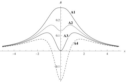
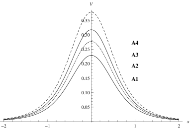
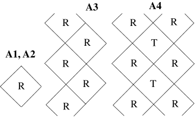
Figure 1: Plots of $B(x)$ (left) and $V(x)$ (right) for symmetric configurations. Curves A1, A2, A3, A4 correspond to $q=0.7,\ 0.77,\ 0.82461,\ 0.9$, respectively. The lower panel shows the Carter-Penrose diagrams of the corresponding space-times.

To begin with, from (16) it follows that $B(x)$ is an even function if and only if $p=0$, hence $m=(2/3)\pi q^{2}$. Then $V(x)$ is also an even function. Such symmetric configurations are asymptotically flat at both ends, $x\to\pm\infty$, and can be classified as follows (see the corresponding curves in Fig. 1):

A1, A2:

Twice asymptotically flat (M-M) wormholes. The curve A2 contains a minimum of $B(x)$ at $x=0$.

A3:

Extremal regular black holes (M-M), with a double horizon (curve A2).

A4:

Non-extremal regular black holes (M-M), with two simple horizons (curve A3).

The abbreviation (M-M) stands here for two flat (Minkowski) asymptotic regions; we will also use similar notations for de Sitter (dS) and anti-de Sitter (AdS) asymptotic behaviors.

The symmetric models form a one-parameter family, depending on $q$; clearly, at $q$ smaller than those appearing in Fig. 1 we also obtain wormholes (the simplest of them is with $q=m=0$ and $V\equiv 0$, it is the Ellis massless wormhole [4, 3]), while at larger $q$ there are non-extremal regular black holes. The critical value of $q$ that separates them is $q\approx 0.825$ (and $m\approx 0.713$), at which there emerges a double horizon corresponding to a double root of $B(x)$, hence a regular extremal BH.

  

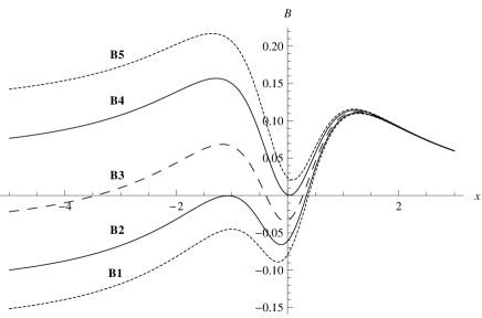
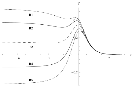
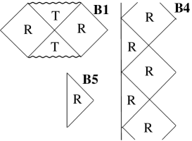
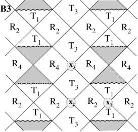
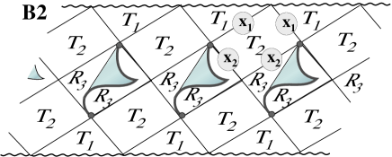
Figure 2: Plots of $B(x)$ (top, left) and $V(x)$ (top, right) for asymmetric configurations at parameter values close to critical ones. The parameters are: $m=0.725$ and $q=0.821,\ 0.8242,\ 0.829,\ 0.835,\ 0.839$ for curves B1–B5, respectively. In the corresponding Carter-Penrose diagrams, the letters R and T label R- and T-regions, respectively, while indices near R and T enumerate ranges with a certain sign of $B(x)$ along the $x$ axis from left to right. The symbols $x_{n}$ enumerate horizons (zeros of $B(x)$) from left to right: $x_{1}<x_{2}<\ldots$. The diagram for B3 occupies the whole plane except the dashed triangles. The diagram for B2 cannot be placed in a plane since there are overlapping regions, as shown in the picture: the $R_{3}$ region drawn below has a flat infinity ($x\to\infty$) on the right, while in another $R_{3}$ region, drawn turned up, such an infinity is on the left.

It is of interest that in the narrow range of $q$ in which the behavior of $B(x)$ drastically changes, the potential $V(x)$ changes very little. We also notice that at large $|x|$ the potential takes small positive values. It is not by chance since in the general case (20) $V(x)$ behaves at large $x$ as follows:

$$V(x)=\frac{4m}{5x^{5}}-\frac{2q^{2}}{3x^{6}}+O(x^{-7}).$$ (22)

3.3 Asymmetric configurations

Concerning asymmetric configurations, it is natural to expect a critical behavior, i.e., transitions between different types of models, at values of $m$ and $q$ close to those appearing in Fig. 2 (but certainly with $p\neq 0$). This idea is confirmed by a direct inspection, and Fig. 2 (left) shows the corresponding five modes of the behavior of $B(x)$ at $m=0.725$:

B1:

A black universe (M-dS) with a single simple horizon.

B2:

A black universe (M-dS) with two horizons (simple and double).

B3:

A black universe (M-dS) with three simple horizons.

B4:

A regular extremal black hole (M-AdS) with a double horizon, asymptotically AdS at the far end ($x\to-\infty$).

B5:

A wormhole (M-AdS), asymptotically AdS at the far end ($x\to-\infty$).

The shape of the potential $V(x)$ (Fig. 3, right) corresponds to Eq. (21): it is certainly zero at the flat asymptotic and is of the opposite sign to that of $B$ at the other end.

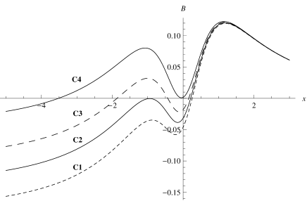
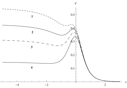
Figure 3: Plots of $B(x)$ (top, left) and $V(x)$ (top, right) for asymmetric configurations with the parameter values $m=0.7$ and $q=0.806,\ 0.8086,\ 0.811,\ 0.8148$ for curves C1–C4, respectively. In the Carter-Penrose diagram for C4 shown below, the notations are the same as in Fig. 2.

A somewhat different picture is observed if we slightly move down the mass and charge values, see Fig. 3 corresponding to $m=0.7$. A qualitatively new feature as compared to Fig. 2 is that the function $B(x)$ corresponding to a double horizon between two R-regions (curve C4) has a negative limit as $x\to-\infty$. As a result, it is a black universe model instead of an M-AdS regular BH. Accordingly, the global causal structure characterized by the Carter-Penrose diagram is quite different (Fig. 3, bottom).

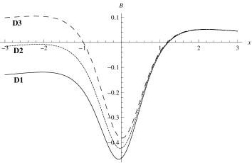
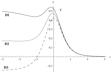
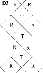
Figure 4: Plots of $B(x)$ (left) and $V(x)$ (middle) for asymmetric configurations with the parameter values $m=1$ and $q=0.968$ (curve D1), $q=0.974$ (curve D2) and $q=0.98$ (curve D3). The right panel shows the Carter-Penrose diagram for D3.

Less diverse is the solution behavior at larger values of the parameters, as exemplified in Fig. 5:

D1, D2:

Black universes (M-dS) with a single simple horizon,

D3:

Regular black holes (M-AdS) with two simple horizons.

The curve D3 corresponds to one more type of global causal structure: the Carter-Penrose diagram (Fig. 4, right) is the same as for a non-extremal Reissner-Nordström BH, but instead of a Reissner-Nordström central singularity we have an AdS infinity.

Figure 5: A symmetric configuration (dS-dS) with four simple horizons, $m=0.739$, $q=0.84$, $B_{0}=-3\pi m/2+\pi^{2}q^{2}/4-0.05$. Plots of $B(x)$ (top, left) and $V(x)$ (top, right) and the Carter-Penrose diagram (bottom), with the same notations as before. The diagram occupies the whole plane except the segments shown by wavy lines (de Sitter infinities).

So far we have been assuming that the space-time is asymptotically flat as $x\to\infty$. It is clear that if we abandon this assumption, then the number of possible qualitatively different globally regular configurations in the scalar-electrovacuum system under consideration will be still larger. To see how they can look, let us note that in Eq. (16) the constant $B_{0}$ is additive. Therefore, changing $B_{0}$, we simply move up or down the plot of $B(x)$, thus changing the asymptotic behavior and the number and nature of horizons in our model. For instance, if we slightly move down the curve A3 in Fig. 2, we obtain a configuration with two de Sitter asymptotics (dS-dS), separated by four simple horizons, see Fig. 5.

In the same way it is easy to obtain a number of other configurations with dS and AdS asymptotic behaviors.

4 Discussion

Scalar-vacuum configurations with a self-interacting phantom scalar field have been considered in [1, 2] (see also references therein); they included M-M and M-AdS wormholes and black universes. In the present paper, we have obtained similar models with an electromagnetic field added and found that its inclusion leads to a greater diversity of qualitatively different configurations. More specifically, even being restricted to solutions which are asymptotically flat as $x\to\infty$ and have $m\geq 0$, we have found as many as 10 types of models, classified by the types of asymptotic behavior and the number and nature of horizons. At zero charge $q$ we return to the situation discussed in [1, 2], with only two configuration types: M-M wormholes with $m=0$ (its analogue is represented here by the curve A1) and black universes with a single simple horizon (a similar behavior of $B(x)$ is shown here, e.g., by the curves B1 and C1); also, M-AdS wormholes were obtained there but only for $m<0$. As already mentioned, the reason for such a narrow choice is that in a pure scalar-vacuum system the field equations forbid the function $B(u)$ to have a regular minimum [16].

Different types of regular configurations obtained here, which are asymptotically flat as $x\to\infty$ and have a nonnegative Schwarzschild mass, are summarized in the table.

Table 1: Types of asymptotically flat solutions with $m>0$

Solution type	Configuration type, asymptotics	Horizons: number, order $n$
(curve number)	($x\to+\infty$) — ($x\to-\infty$)	[disposition of R- and T-regions]
A1,A2	M - M wormhole	none [R]
A3	M - M extremal black hole	1 hor., $n=2$ [RR]
A4	M - M black hole	2 hor., $n=1$ (both) [RTR]
B1, C1, C4, D1, D2	M - dS black universe	1 hor., $n=1$ [TR]
B2, C2	M - dS black universe	2 hor., $n=2$ and $n=1$ [TTR]
C4	M - dS black universe	2 hor., $n=1$ and $n=2$ [TRR]
B3, C3	M - dS black universe	3 hor., $n=1$ (for all), [TRTR]
D3	M - AdS black hole	2 hor., $n=1$ [RTR]
B4	M - AdS extremal black hole	1 hor., $n=2$ [RR]
B5	M - AdS wormhole	none [R]

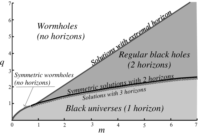
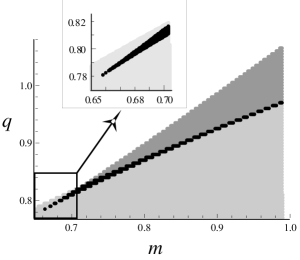
Figure 6: Map of asymptotically flat solutions with $m>0$. Right panel: a domain of interest enlarged

The general landscape of our solutions with a flat infinity on the right end and a positive Schwarzschild mass can be characterized by a map drawn in the $(m,q)$ plane (Fig. 6). It can be seen that the most generic are M-AdS wormhole solutions and black universes with a single simple horizon: they exist for all values of $m$ and are actually the same types of solutions that have been obtained before with $q=0$ [1]. One more generic type of models is formed by regular BHs with two horizons, which appear only with sufficiently large charges. Solutions with extremal horizons appear on separatrices between the main domains on the plane, while solutions with three simple horizons are also generic since they occupy a certain area on the plane, but this area is actually a very narrow band, it is almost invisible if we do not specially adjust the scale, see the right panel in Fig. 6.

We conclude that the present field system creates quite a number of diverse models, making us substantially widen the list of possible regular BH configurations as compared, e.g., with [2]. Such models can be of interest both as descriptions of local objects (black holes, wormholes) and as a basis for building singularity-free cosmological scenarios. An important feature of such cosmologies, different from the great majority of nonsingular models described in the literature, is that the cosmological expansion starts from a Killing horizon (this phenomenon can be termed a Null Big Bang [19, 20]) beyond which, in the absolute past, there is an asymptotically flat static region. There is another kind of configurations with a Null Big Bang where a static region, instead, contains a regular center [19, 21]; as in the present paper, the models described there can possess multiple horizons and have a de Sitter asymptotic behavior at late times.

An important point concerns the value of the global magnetic field that exists in our Universe if it can be described by a model more or less like ours. Let us use the (probably) most conservative estimate, according to which a lower limit on the magnetic field strength is $B\gtrsim 10^{-18}$ G [22]. On the other hand, the present scale factor $a_{0}\approx 10^{28}$ cm approximately coincides with the quantity $r(u)$ in the metric (2). Therefore, since $B\propto r^{-2}$ [see (6)], we can roughly estimate the field values at earlier stages of the evolution. For instance, at recombination ($a/a_{0}\sim 10^{-3}$), when the electromagnetic radiation decoupled from matter, the magnetic field was still weak enough, $B\sim 10^{-12}$ G, but at the stage of baryogenesis ($a/a_{0}\sim 10^{-12}$) it was of the order of $10^{6}$ G.

Observations of the cosmic microwave background (CNB) show that our Universe is highly isotropic: at recombination, the degree of anisotropy did not exceed $10^{-6}$. If this condition holds, spherically symmetric models like ours (belonging to the Kantowski-Sachs class), being anisotropic by construction, can still conform to observations [23].

The above condition constrains the global magnetic field strength allowed by the observed CMB isotropy. The CMB energy density $\rho_{\rm CMB}$ and that of the the magnetic field, $\rho_{\rm magn}$, are both proportional to $r^{-4}$ as long as the Universe is approximately isotropic, hence their ratio is constant and is the same at recombination and at present. But at present $\rho_{\rm CMB}\sim 10^{-33}$ ${\rm g/cm^{3}}$, hence we should require $\rho_{\rm magn}\lesssim 10^{-39}$ ${\rm g/cm^{3}}$, which in turn means $|B|\lesssim 10^{-8}$ G. We see that this condition is easily satisfied by the fields under consideration.

An upper limit on the classical magnetic field description seems to follow from the work of Ambjorn and Olesen [24] who pointed out that the Weinberg-Salam model of electroweak interactions shows an instability at $B\gtrsim 10^{24}$ G, connected with emergence of a tachyonic mode. If at present $|B|\sim 10^{-18}$ G, then the maximum admissible value of $B$ corresponds to $r\approx 10^{7}$ cm $=100$ km — it is the minimum admissible value of $b=\min r(u)$ in our models.

The possible viability of models like those considered in this paper depends on their stability under various kinds of perturbations. Most of the known scalar-vacuum wormhole and black-universe solutions proved to be unstable under radial perturbations [25, 26, 27], and it is of interest to find out whether or not they can be stabilized by electric or magnetic fields. We hope to consider this problem in the near future.

Acknowledgments

This work was supported in part by NPK MU grant at PFUR and by FTsP “Nauchnye i nauchno-pedagogicheskie kadry innovatsionnoy Rossii” for the years 2009-2013.

References

- [1] K.A. Bronnikov and J.C. Fabris, Phys. Rev. Lett. 96, 251101 (2006); gr-qc/0511109.
- [2] K.A. Bronnikov, V.N. Melnikov and H. Dehnen, Gen. Rel. Grav. 39, 973 (2007); gr-qc/0611022.
- [3] K.A. Bronnikov, Acta Phys. Pol. B4, 251 (1973).
- [4] H. Ellis, J. Math. Phys. 14, 104 (1973).
- [5] F.S.N. Lobo, in: Classical and Quantum Gravity Research ed. C.N. Mikkel and T.K. Rasmussen (Hauppauge, NY: Nova Science, 2008), pp. 1–78; ArXiv: 0710.4474.
- [6] K.A. Bronnikov and S.G. Rubin, Lectures on Gravitation and Cosmology (MIFI press, Moscow, 2008, in Russian).
- [7] E. Komatsu, Astrophys. J. Suppl. 192, 18 (2011).
- [8] M. Sullivan at al., Astrophys. J. 737, 102 (2011); Arxiv: 1104.1444.
- [9] R. Gannouji, D. Polarski, A. Ranquet and A.A. Starobinsky, JCAP 0609, 016 (2006); astro-ph/0606287.
- [10] R.R. Caldwell, M. Kamionkowski and N.N. Weinberg, Phys. Rev. Lett. 91, 071301 (2003); astro-ph/0302506.
- [11] K.A. Bronnikov and E.V. Donskoy, Grav. Cosmol. 16, 42 (2010); ArXiv: 0910.4930.
- [12] R. Poltis and D. Stojkovic, Phys. Rev. Lett. 105, 161301 (2010); arXiv: 1004.2704.
- [13] J.A. Wheeler, Phys. Rev. 97, 511 (1955).
- [14] M.S. Morris and K.S. Thorne, Am. J. Phys. 56, 395 (1988).
- [15] R. Penney, Phys. Rev. 182, 1383 (1969).
- [16] K.A. Bronnikov, Phys. Rev. D 64, 064013 (2001); gr-qc/0104092.
- [17] K.A. Bronnikov and S.V. Sushkov, Class. Quantum Grav. 27, 095022 (2010); ArXiv: 1001.3511.
- [18] K.A. Bronnikov and E.V. Donskoy, Grav. Cosmol. 17, 176 (2011); arXiv: 1110.6030.
- [19] K.A. Bronnikov and I.G. Dymnikova, Class. Quantum Grav. 24, 5803–5816 (2007); Arxiv: 0705.2368.
- [20] K.A. Bronnikov and O.B. Zaslavskii, Class. Quantum Grav. 25, 105015 (2008); ArXiv: 0710.5618.
- [21] K.A. Bronnikov, I.G. Dymnikova and E. Galaktionov, Class. Quantum Grav. 29, 095025 (2012); ArXiv: 1204.0534.
- [22] C.D. Dermer et al., ArXiv: 1011.6660.
- [23] P. Aguiar and P. Crawford, Phys. Rev. D 62, 123511 (2000).
- [24] J. Ambjorn and P. Olesen, Nucl. Phys. B 315, 606 (1989); Int. J. Mod. Phys.A 5, 4525 (1990).
- [25] J.A. Gonzalez, F.S. Guzman, and O. Sarbach, Class. Quantum Grav. 26, 015010 (2009); Arxiv: 0806.0608.
- [26] K.A. Bronnikov, J.C. Fabris, and A. Zhidenko, Eur. Phys. J. C 71, 1791 (2011).
- [27] K.A. Bronnikov, R.A. Konoplya, and A. Zhidenko, Phys. Rev. D 86, 024028 (2012).