Modeling a falling slinky

Abstract

A slinky is an example of a tension spring: in an unstretched state a slinky is collapsed, with turns touching, and a finite tension is required to separate the turns from this state. If a slinky is suspended from its top and stretched under gravity and then released, the bottom of the slinky does not begin to fall until the top section of the slinky, which collapses turn by turn from the top, collides with the bottom. The total collapse time $t_{c}$ (typically $\sim 0.3$ s for real slinkies) corresponds to the time required for a wave front to propagate down the slinky to communicate the release of the top end. We present a modification to an existing model for a falling tension spring calkin93 and apply it to data from filmed drops of two real slinkies. The modification of the model is the inclusion of a finite time for collapse of the turns of the slinky behind the collapse front propagating down the slinky during the fall. The new finite-collapse time model achieves a good qualitative fit to the observed positions of the top of the real slinkies during the measured drops. The spring constant $k$ for each slinky is taken to be a free parameter in the model. The best-fit model values for $k$ for each slinky are approximately consistent with values obtained from measured periods of oscillation of the slinkies.

I Introduction

The physics of slinkies has attracted attention since their invention in 1943. Topics of studies include the hanging configuration of the slinky, mak87 ; sawicki2002 the ability of a slinky to walk down stairs, hu2010 the modes of oscillation of a vertically suspended slinky, bowen82 ; young93 the dispersion of waves propagating along slinkies,blake79 ; crawford87 ; vandegrift89 and the behavior of a vertically stretched slinky when it is dropped. calkin93 ; aguirregabiria2007 ; unruh2011

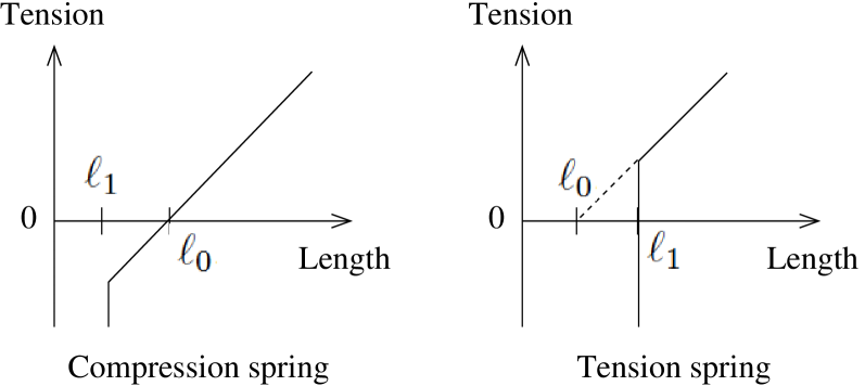
Fig. 1: Tension versus length diagrams for a compression spring (left) and a tension spring (right). The tension in each spring is zero for spring length $\ell_{0}$ assuming Hooke’s law applies (this length is not achieved for the tension spring). The turns of the spring touch for length $\ell_{1}$.

Slinkies are examples of tension springs, i.e. springs which may be under tension according to Hooke’s law, but not compression. Unstretched slinkies have a length $\ell_{1}$ at which the turns are in contact, and a finite tension $f_{1}$ is needed to separate the turns from this state. They collapse to this state if not stretched by an external force. This may be contrasted with a “compression spring,” which can be under tension or compression according to Hooke’s law. Compression springs have an unstretched length $\ell_{0}$ at which the turns are not in contact, and the tension is zero. They may be compressed to a length $\ell_{1}$ at which the turns are in contact, and obey Hooke’s law during this compression. Fig. 1 shows tension versus length diagrams for uniform extensions of the two types of springs.

The vertically falling slinky, mentioned above, exhibits interesting dynamics which depend on the slinky being a tension spring. calkin93 A falling compression spring exhibits periodic compressions and rarefactions, as longitudinal waves propagate along the spring length. A falling tension spring collapses to the length $\ell_{1}$ during a fall, assuming the spring is released in an initially stretched state (with length $>\ell_{1}$).

If a slinky is hanging vertically under gravity from its top (at rest) and then released, the bottom of the slinky does not start to move downwards until the collapsing top section collides with the bottom. Figure 2 illustrates this peculiar effect for a plastic rainbow-colored slinky; this figure shows a succession of frames extracted from a high-speed video of the fall of the slinky. wheatland_cross12 The continued suspension of the bottom of the slinky after release is somewhat counter-intuitive and very intriguing—a recent YouTube video showing the effect with a falling slinky has received more than 800,000 views. muller_cross10 The physical explanation is straightforward: the collapse of tension in the slinky occurs from the top down, and a finite time is required for a wave front to propagate down the slinky communicating the release of the top.

The basic wave physics behind this behavior follows from the equation of motion for a falling (or suspended) compression springedwards72

$$m\frac{\partial^{2}x}{\partial t^{2}}=k\frac{\partial^{2}x}{\partial\xi^{2}}+mg,$$ (1)

which applies to a tension spring when the turns are separated. In this equation $x(\xi,t)$ is the vertical location of a point along the spring at time $t$, $m$ is the total spring mass, and $k$ is the spring constant. The (dimensionless) coordinate $\xi$ describes the mass distribution along the spring, such that $dm=m\,d\xi$ is the increment in mass associated with an increment in $\xi$, with $0\leq\xi\leq 1$. Thus, for a spring with $N$ turns, the end of turn $i$ corresponds to $\xi_{i}=i/N$ and is located at position $x_{i}=x(\xi_{i},t)=x(i/N,t)$ at time $t$. Equation (1) is an inhomogenous wave equation. If the spring is falling under gravity, then in a coordinate system falling with the center of mass of the spring ($x^{\prime}=x-\frac{1}{2}gt^{2}$), the equation of motion is the usual wave equation

$$m\frac{\partial^{2}x^{\prime}}{\partial t^{2}}=k\frac{\partial^{2}x^{\prime}}{\partial\xi^{2}}.$$ (2)

Equation (2) implies that waves in the mass distribution (turn spacing) propagate along the length of the spring in a characteristic time $t_{p}=\sqrt{m/k}$. This accounts for the periodic rarefactions and compressions of a compression spring during a fall, and for the propagation of the wave front ahead of the collapsing turns in a falling tension spring.

In this paper we present a new detailed model for the fall of a slinky, which improves on past models by taking into account the finite time for collapse of the turns of the slinky behind the wave front. In Sec. II we explain the need for this refinement in the modeling, and we present the details of the new model in Sec. III. The new model is compared with the behavior of two real falling slinkies in Sec. IV, and we discuss our conclusions in Sec. V.

II The collapse of the turns at the top of the slinky

A detailed description of the dynamical behavior of a falling tension spring requires solution of the equations of motion for mass elements along the slinky that are subject to gravity and local spring forces, taking into account the departure from Hooke’s law encountered when slinky turns come into contact. Because of the complexity of this modeling, past efforts involve specific approximations. calkin93 ; aguirregabiria2007 ; unruh2011

For a mass element $m\Delta\xi$ at a location $\xi_{i}$ on the slinky, the equation of motion isedwards72

$$\begin{split}m\Delta\xi\left.\frac{\partial^{2}x}{\partial t^{2}}\right|_{\xi_{i},t}&=f(\xi_{i}+\Delta\xi,t)-f(\xi_{i},t)+m\Delta\xi g\\ &=\Delta\xi\left.\frac{\partial f}{\partial\xi}\right|_{\xi_{i},t}+m\Delta\xi g,\end{split}$$ (3)

where $f(\xi,t)$ is the tension force at $\xi$. Equation (3) applies to all points except the top and bottom of the slinky, where the tension is one sided. When slinky turns are separated at a point along the slinky, the tension is given by Hooke’s law in the formcalkin93

$$f(\xi,t)=k\left(\frac{\partial x}{\partial\xi}-\ell_{0}\right),$$ (4)

where $\partial x/\partial\xi$ describes the local extension of the slinky, and $\ell_{0}$ corresponds to a slinky length at which the tension would be zero, assuming a Hooke’s law relation for all values of the local extension. Substituting Eq. (4) into Eq. (3) leads to the inhomogenous wave equation (1).

For a tension spring the length $\ell_{0}$ cannot be reached because there is a minimum length

$$\frac{\partial x}{\partial\xi}=\ell_{1}>\ell_{0}$$ (5)

that corresponds to the spring coils being in contact with each other. At this point, the minimum tension

$$f_{1}=k(\ell_{1}-\ell_{0})$$ (6)

is achieved and the tension is replaced by a large (infinite) compression force as the collapsed turns resist further contraction of the slinky (see Fig. 1). This non-Hooke’s law behavior is met when turns collapse at the top of the falling slinky and the description of this process complicates the modeling.

A simpler, approximate description of the dynamical collapse of the top of the slinky is to assume a functional form for the position-mass distribution $x(\xi,t)$ during the collapse, and then impose conservation of momentum to ensure physical time evolution. Calkin calkin93 introduced this semi-analytic approach and specifically assumed a distribution corresponding to slinky turns collapsing instantly behind a downward propagating wave front located a mass fraction $\xi_{c}=\xi_{c}(t)$ along the slinky at time $t$ after the release. The turns of the slinky at the front instantly assume a configuration with a minimum tension, so that Eq. (5) applies for all points behind the front at a given time

$$f(\xi<\xi_{c},t)=f_{1}.$$ (7)

For points ahead of the front ($\xi>\xi_{c}$) the tension is the same as in the hanging slinky. The location of the front at time $t$ is obtained by requiring that the total momentum of the collapsing slinky matches the impulse imparted by gravity up to that time. (The modeling is presented in detail in Sec. III.2.) The Calkin model has also been derived in solving the inhomogenous wave equation (1) subject to the boundary condition given by Eq. (7). aguirregabiria2007 ; unruh2011

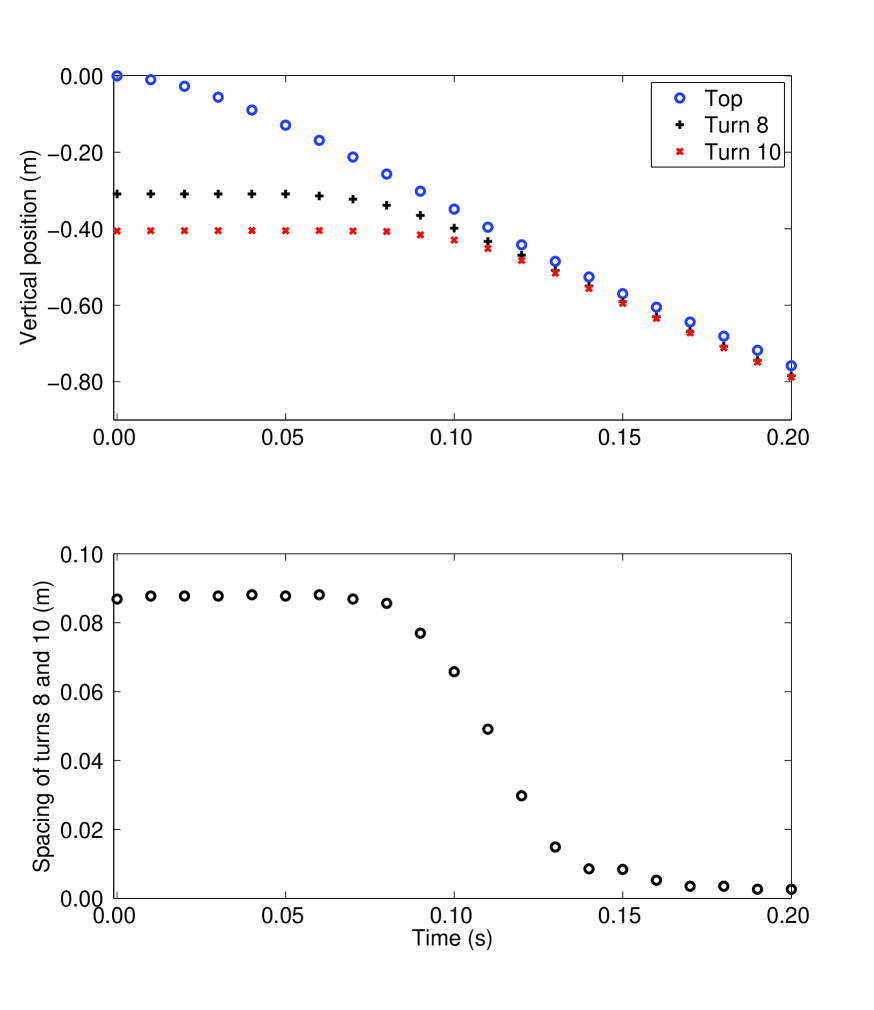
Fig. 3: Data extracted from the video shown in Fig. 2, illustrating the finite time for collapse of the turns of the slinky. Upper panel: position versus time of the top of the slinky (circles, blue online), turn eight of the slinky ($+$ symbols, black online) and turn ten of the slinky ($\times$ symbols, red online). Position is negative downwards in this panel. Lower panel: The spacing of turns eight and ten versus time.

With real falling slinkies the collapse of turns behind the front takes a finite time. Figure 3 illustrates the process of collapse of a real slinky using data extracted from a high-speed video of a fall (this data is discussed in more detail in Sec. IV.1.) The upper panel of Fig. 3 shows the position of the top (blue circles), of turn eight (black $+$ symbols), and of turn ten (red $\times$ symbols) versus time, for the first $0.2$ s of the fall. The vertical position is shown as negative in the downward direction measured from the initial position of the top [which corresponds to $-x$ in terms of the notation of Eq. (2)]. The upper panel shows that turns 8 and 10 of the slinky remain at rest until the top has fallen some distance, and then turn eight begins to fall before turn ten. The lower panel shows the spacing of turns eight and ten versus time. The two turns change from the initial stretched configuration to the final collapsed configuration in $\sim 0.1$ s.

This paper presents a method of solution of Eq. (1) which adopts the approximate approach of Calkin, but includes a finite time for collapse of the turns. We assume a linear profile for the decay in tension behind the wave front propagating down the slinky, which provides a more realistic description of the slinky collapse.

III Modeling the fall of a slinky

In Secs. III.1 and III.2 we reiterate the Calkin calkin93 model for a hanging slinky as a tension spring, and for the fall of the tension spring. In Sec. III.3 the new model for the fall of the slinky is presented.

III.1 The hanging slinky

For hanging slinkies it is generally observed that the top section of the slinky has stretched turns, and a small part at the bottom has collapsed turns. mak87 Assuming mass fractions $\xi_{1}$ and $1-\xi_{1}$ of the slinky with stretched and collapsed turns, respectively, the number of collapsed turns $N_{c}$ is related to the total number of turns $N$ by

$$N_{c}=(1-\xi_{1})N.$$ (8)

A hanging slinky such that the turns just touch at the bottom would have $\xi_{1}=1$.

The position $X=X(\xi)$ of points along the stretched part of the stationary hanging slinky is described by setting $\partial^{2}x/\partial t^{2}=0$ in Eq. (1) and integrating from $\xi=0$ to $\xi=\xi_{1}$ with the boundary conditions

$$X(\xi=0)=0\quad\mbox{and}\quad\left.\frac{\partial X}{\partial\xi}\right|_{\xi=\xi_{1}}=\ell_{1},$$ (9)

corresponding to the fixed location of the top of the slinky, and the spacing of collapsed turns at the bottom of the slinky, respectively. The position of points in the collapsed section at the bottom is obtained by integrating Eq. (5) from $\xi=\xi_{1}$ to $\xi=1$, with the boundary value $X(\xi_{1})$ matching the result obtained by the first integration. Carrying out these calculations gives

$$X(\xi)=\begin{cases}\ell_{1}\xi+\displaystyle{\frac{mg}{k}}\left(\xi_{1}-\frac{1}{2}\xi\right)\xi,&\mbox{for }0\leq\xi\leq\xi_{1}\\ \ell_{1}\xi+\displaystyle{\frac{mg}{2k}}\xi_{1}^{2},&\mbox{for }\xi_{1}\leq\xi\leq 1.\end{cases}$$ (10)

The total length of the slinky in this configuration is

$$X_{\mathrm{B}}=X(1)=\ell_{1}+\frac{mg}{2k}\xi_{1}^{2},$$ (11)

where B refers to the bottom of the slinky, and the center of mass is at

$$X_{\mathrm{com}}=\int_{0}^{1}X(\xi)\,d\xi=\frac{1}{2}\ell_{1}+\frac{mg}{2k}\left(1-\frac{1}{3}\xi_{1}\right)\xi_{1}^{2}.$$ (12)

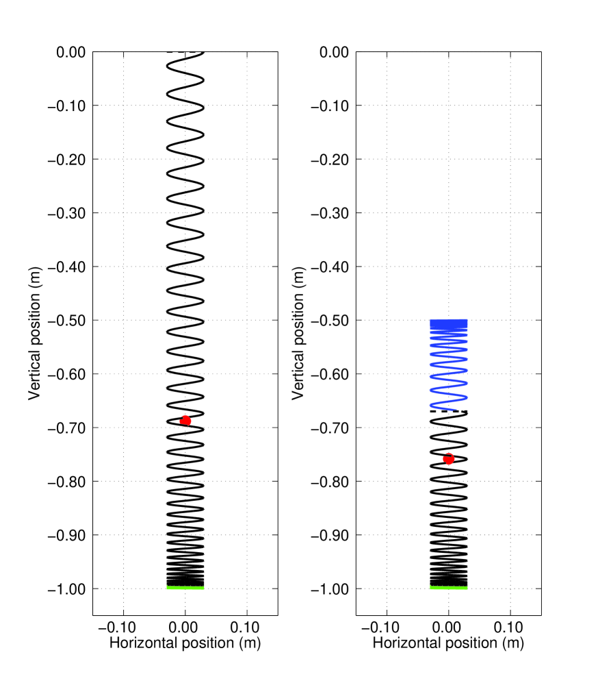
Fig. 4: Left panel: the model for a hanging slinky, with the slinky represented as a helix with turn spacing matching $X(\xi)$. Typical slinky parameters are used. The dot in each panel indicates the location of the center of mass, and the light gray (green online) part of the slinky at the bottom is the collapsed section. Right panel: the finite-collapse-time model for the slinky during the fall at time $t=t_{c}/2$. The top dark gray (blue online) section of the slinky is the section undergoing collapse, above the downward-propagating collapse front indicated by a dashed horizontal line.

The left panel of Fig. 4 illustrates the model slinky in the hanging configuration. The slinky is drawn as a helix with a turn spacing matching $X(\xi)$, for model parameter values typical of real slinkies (detailed modeling of real slinkies is presented in Sec. IV). The chosen parameters are: $80$ total turns ($N=80$), slinky mass $m=200$ g, hanging length $X_{\mathrm{B}}=1$ m, collapsed length $\ell_{1}=60$ mm, slinky radius $30$ mm, and $10\%$ of the slinky mass collapsed at the bottom when hanging ($\xi_{1}=0.9$). The light gray (green online) section of the slinky at the bottom is the collapsed section, and the dot (red online) is the location of the center-of-mass of the slinkey (given by Eq. (12) in the left panel).

III.2 The falling slinky with instant collapse of turns

We assume the slinky is released at $t=0$ and the turns collapse from the top down behind a propagating wave front. In the model with instant collapse calkin93 the process is completely described by the location $\xi_{c}=\xi_{c}(t)$ of the front at time $t$. The slinky is collapsed where $0\leq\xi<\xi_{c}$ but is still in the initial state where $\xi_{c}<\xi\leq 1$. The position of points in the collapsed section of the slinky, behind the front, is obtained by integrating Eq. (5) and matching to the boundary condition

$$x(\xi=\xi_{c},t)=X(\xi_{c}),$$ (13)

to get

$$x(\xi,t)=\ell_{1}\xi+\frac{mg}{k}\xi_{c}\left(\xi_{1}-\frac{1}{2}\xi_{c}\right)$$ (14)

for $0\leq\xi\leq\xi_{c}$. The lower part of the slinky ($\xi_{c}\leq\xi\leq 1$) has positions described by Eq. (10).

The motion of the slinky after release follows from Newton’s second law. The collapsed top section has a velocity given by the derivative of Eq. (14)

$$\frac{\partial x(\xi,t)}{\partial t}=\frac{mg}{k}\left(\xi_{1}-\xi_{c}\right)\frac{d\xi_{c}}{dt},$$ (15)

and the mass of this section is $m\xi_{c}$. The rest of the slinky is stationary so the total momentum of the slinky is obtained by multiplying Eq. (15) by the mass $m\xi_{c}$. Setting the momentum equal to the net impulse $mgt$ due to gravity on the slinky at time $t$ gives

$$\xi_{c}\left(\xi_{1}-\xi_{c}\right)\frac{d\xi_{c}}{dt}=\frac{k}{m}t,$$ (16)

which can be directly integrated to give

$$\xi_{c}^{2}\left(\xi_{1}-\frac{2}{3}\xi_{c}\right)=\frac{k}{m}t^{2}.$$ (17)

At a given time Eq. (17) is a cubic in $\xi_{c}$; the first positive root to the cubic defines the location of the collapse front at that time. The total collapse time $t_{c}$—the time for the collapse front to reach the bottom, collapsed section—is defined by $\xi_{c}(t_{c})=\xi_{1}$, and from Eq. (17) it follows that

$$t_{c}=\sqrt{\frac{m}{3k}\xi_{1}^{3}}\,.$$ (18)

Equation (17), together with Eqs. (10) and (14), defines the location $x(\xi,t)$ of all points on the slinky for $t<t_{c}$. The center of mass falls from rest with acceleration $g$ and so has location

$$x_{\mathrm{com}}(t)=X_{\mathrm{com}}+\frac{1}{2}gt^{2},$$ (19)

where $X_{\mathrm{com}}$ is given by Eq. (12).

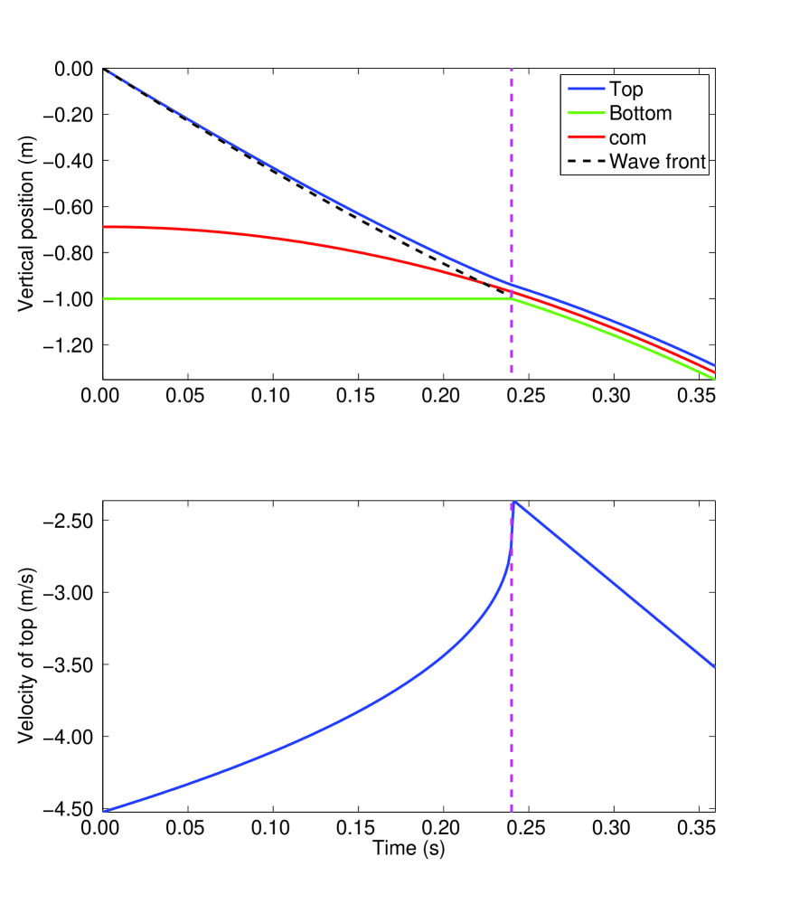
Fig. 5: The instant-collapse model calkin93 for a falling slinky using parameters typical of a real slinky. Upper panel: position versus time of the slinky top (upper solid curve), center-of-mass (middle solid curve), bottom (lower solid curve), and wave front initiating collapse (dashed curve). Position is negative downwards in this figure. Lower panel: velocity of the slinky top versus time. The total collapse time $t_{c}$ is shown as the vertical dashed line in both panels.

Figure 5 shows solution of the instant-collapse model with the typical slinky parameters used in Fig. 4. wheatland_cross12 The upper panel shows the positions of the top (upper solid curve, blue online), center-of-mass (middle solid curve, red online), and bottom (lower solid curve, red online) of the slinky versus time. Position is negative in the downward direction so the upper (blue) curve corresponds to the model expression $-x(0,t)$. The position of the front versus time is indicated by the dashed (black) curve. The lower panel shows the velocity of the top of the slinky versus time (solid curve, blue online) and in both panels the total collapse time $t_{c}$ is indicated by the vertical dashed (pink) line. For the typical slinky parameters used, the spring constant is $k=0.84$ N/m and the collapse time is $t_{c}\approx 0.24$ s.

Figure 5 illustrates a number of unusual features of the model. For example, the initial velocity of the top is non-zero—a consequence of the assumption of instant collapse at the wave front. From Eqs. (15) and (17) the initial velocity of the top is

$$v_{T}^{0}=-\left.\frac{\partial x}{\partial t}\right|_{\xi=0}=-g\sqrt{\frac{m\xi_{1}}{k}}\approx-4.5\,\mathrm{m/s}.$$ (20)

The acceleration of the top at time $t=0$ must be infinite to produce a finite initial velocity. The acceleration of the top of the slinky just after $t=0$ is positive, i.e. in the upwards direction, so the top of the slinky falls more slowly with time. From Eqs. (15) and (17) the limiting value of the acceleration as $t\rightarrow 0$ is

$$a_{T}^{0}=-\left.\frac{\partial^{2}x}{\partial t^{2}}\right|_{\xi=0}=\frac{g}{3\xi_{1}}\approx 3.6\,\mathrm{m/s}^{2}.$$ (21)

The acceleration of the top becomes negative (downwards) after the collision of the top and bottom sections, when the whole slinky falls with acceleration $-g$. At the collapse time when the top section impacts the bottom section there is an impulsive collision causing a discontinuous jump in the velocity.

III.3 The falling slinky with a finite time for collapse of turns

The instant-collapse model requires an unphysical instant change in the angle of the slinky turns behind the collapse front, as discussed in Secs. II and III.2. This affects the positions of all turns of the slinky as a function of time behind the front. To model the positions of the turns of a real collapsing slinky it is necessary to modify the model.

The lower panel of Fig. 3 indicates that the spacing between the turns of the slinky decreases approximately linearly with time during the collapse. Hence we modify the model in Sec. III.3 to include a linear profile for the decay in tension behind the collapse front propagating down the slinky, as a function of mass fraction $\xi$. The tension is assumed to be given by Eq. (4) with

$$\frac{\partial x}{\partial\xi}=\left[X^{\prime}(\xi_{c})-\ell_{1}\right]\left(1+\frac{\xi-\xi_{c}}{\Delta}\right)+\ell_{1}\quad\mathrm{for}~{}\mathrm{max}(0,\xi_{c}-\Delta)\leq\xi\leq\xi_{c},$$ (22)

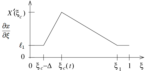
Fig. 6: The gradient $\partial x/\partial\xi$, which describes the local slinky extension, versus mass density $\xi$ in the finite-collapse-time model. The tension defined by this profile declines linearly behind the wave front [located at $\xi_{c}(t)$] from a value matching the tension in the hanging slinky at the front, to the minimum tension value $f_{1}=k(\ell_{1}-\ell_{0})$ at $\xi=\xi_{c}-\Delta$. Ahead of the front the tension is unchanged from that in the hanging slinky.

where $X=X(\xi)$ is given by Eq. (10), and the prime denotes differentiation with respect to the parameter $\xi$. In this equation, $\Delta$ is a parameter that governs the distance over which the tension decays back to its minimum value $f_{1}$. Figure 6 illustrates the local slinky extension at time $t$ as described by Eq. (22). Behind the front at $\xi_{c}(t)$ the extension decreases linearly as a function of $\xi$, returning to the minimum value $\ell_{1}$ over the fixed mass fraction $\Delta$. Ahead of the front the extension is the same as for the hanging slinky.

Equation (22) replaces Eq. (5) for the section of the slinky behind the collapse front and provides a simple, approximate description of a finite collapse time for the turns behind the front. The limit $\Delta\rightarrow 0$ in the new model recovers the instant-collapse model.

Using Eq. (10) to evaluate the gradient in Eq. (22) gives

$$\frac{\partial x}{\partial\xi}=\frac{mg}{k}\left(\xi_{1}-\xi_{c}\right)\left(1+\frac{\xi-\xi_{c}}{\Delta}\right)+\ell_{1}\quad\mathrm{for}~{}\mathrm{max}(0,\xi_{c}-\Delta)\leq\xi\leq\xi_{c}.$$ (23)

Integrating Eq. (23) and imposing the boundary condition $x(\xi_{c})=X(\xi_{c})$ using Eq. (10) gives

$$x=\frac{mg}{k}\left[\left(\xi_{1}-\xi_{c}\right)\left(1-\frac{1}{\Delta}\xi_{c}+\frac{1}{2\Delta}\xi\right)\right]\xi+\ell_{1}\xi+\frac{mg}{2k}\xi_{c}^{2}\left(1+\frac{\xi_{1}-\xi_{c}}{\Delta}\right)$$ (24)

for $\mathrm{max}(0,\xi_{c}-\Delta)\leq\xi\leq\xi_{c}$. If $\xi_{c}>\Delta$, there is a completely collapsed section at the top of the slinky. The mass density in this section is obtained by integrating Eq. (5) and matching to the value $x(\xi_{c}-\Delta)$ given by Eq. (24), leading to

$$x=\ell_{1}\xi+\frac{mg}{k}\left[\xi_{c}\left(\xi_{1}-\frac{1}{2}\xi_{c}\right)-\frac{1}{2}\Delta\left(\xi_{1}-\xi_{c}\right)\right]\quad\mathrm{for}~{}0\leq\xi\leq\mathrm{max}(0,\xi_{c}-\Delta).$$ (25)

Equations (24) and (25) are the counterparts to Eq. (14) in the instant-collapse model. In the limit $\Delta\rightarrow 0$, Eq. (25) is the same as Eq. (14).

The motion of the slinky in the new model is determined in the same way as for the instant-collapse model. The velocity of the top section of the slinky prior to the complete collapse of the top is obtained by differentiating Eqs. (24) and (25) to get

$$\begin{split}\frac{\partial x}{\partial t}=\frac{mg}{k}&\left[\left(1+\frac{\xi_{1}-3\xi_{c}/2}{\Delta}\right)\xi_{c}-\left(1+\frac{\xi_{1}-2\xi_{c}+\xi/2}{\Delta}\right)\xi\right]\frac{d\xi_{c}}{dt},\\ &\quad\quad\mathrm{for}~{}\mathrm{max}(0,\xi_{c}-\Delta)\leq\xi\leq\xi_{c},\end{split}$$ (26)

and

$$\frac{\partial x}{\partial t}=\frac{mg}{k}\left(\xi_{1}-\xi_{c}+\frac{1}{2}\Delta\right)\frac{d\xi_{c}}{dt},\quad\mathrm{for}~{}0\leq\xi\leq\mathrm{max}(0,\xi_{c}-\Delta).$$ (27)

Equation (27) is the counterpart to Eq. (15). The total momentum of the slinky is given by

$$p=m\int_{0}^{\xi_{c}}\frac{\partial x}{\partial t}d\xi\,,$$ (28)

and using Eqs. (26) and (27) to evaluate the integral gives

$$p=\frac{m^{2}g}{2k}\xi_{c}^{2}\left(1+\frac{\xi_{1}-4\xi_{c}/3}{\Delta}\right)\frac{d\xi_{c}}{dt}\quad\mathrm{if}~{}\xi_{c}\leq\Delta,$$ (29)

and

$$p=\frac{m^{2}g}{k}\left[\xi_{c}\left(\xi_{1}-\xi_{c}\right)+\Delta\left(\xi_{c}-\frac{1}{2}\xi_{1}-\frac{1}{6}\Delta\right)\right]\frac{d\xi_{c}}{dt}\quad\mathrm{if}~{}\xi_{c}\geq\Delta.$$ (30)

Setting Eqs. (29) and (30) equal to the total impulse $mgt$ on the slinky up to time $t$ gives equations defining the location $\xi_{c}(t)$ of the front at time $t$:

$$\frac{1}{2}\xi_{c}^{2}\left(1+\frac{\xi_{1}-\frac{4}{3}\xi_{c}}{\Delta}\right)\frac{d\xi_{c}}{dt}=\frac{kt}{m}\quad\mathrm{if}~{}\xi_{c}\leq\Delta,$$ (31)

and

$$\left[\xi_{c}\left(\xi_{1}-\xi_{c}\right)+\Delta\left(\xi_{c}-\frac{1}{2}\xi_{1}-\frac{1}{6}\Delta\right)\right]\frac{d\xi_{c}}{dt}=\frac{kt}{m}\quad\mathrm{if}~{}\xi_{c}\geq\Delta,$$ (32)

which are the counterparts to Eq. (16) in the instant-collapse model. Equations (31) and (32) may be integrated with respect to $\xi_{c}$, leading to

$$\xi_{c}^{3}\frac{\Delta+\xi_{1}-\xi_{c}}{3\Delta}=\frac{kt^{2}}{m}\quad\mathrm{if}~{}\xi_{c}\leq\Delta,$$ (33)

and

$$\xi_{c}^{2}\left(\xi_{1}-\frac{2}{3}\xi_{c}\right)-\Delta\left(\xi_{1}-\xi_{c}\right)\left(\xi_{c}-\frac{1}{3}\Delta\right)=\frac{kt^{2}}{m}\quad\mathrm{if}~{}\xi_{c}\geq\Delta,$$ (34)

which are the counterparts to Eq. (17) that defines the location of the front in the instant-collapse model.

The total collapse time $t_{c}$ for the slinky (the time for the front to reach $\xi_{1}$) is obtained by setting $\xi_{c}=\xi_{1}$ in Eq. (34). Interestingly, the result is unchanged from the instant-collapse case and is given by Eq. (18). A second time scale relevant for the model is the time $t_{\mathrm{lin}}$ for the top of the slinky to undergo the initial linear collapse (for times $t>t_{\mathrm{lin}}$ there are completely collapsed turns at the top of the slinky). This is obtained by setting $\xi_{c}=\Delta$ in Eq. (33) to get

$$t_{\mathrm{lin}}=\sqrt{\frac{m\xi_{1}}{3k}}\Delta.$$ (35)

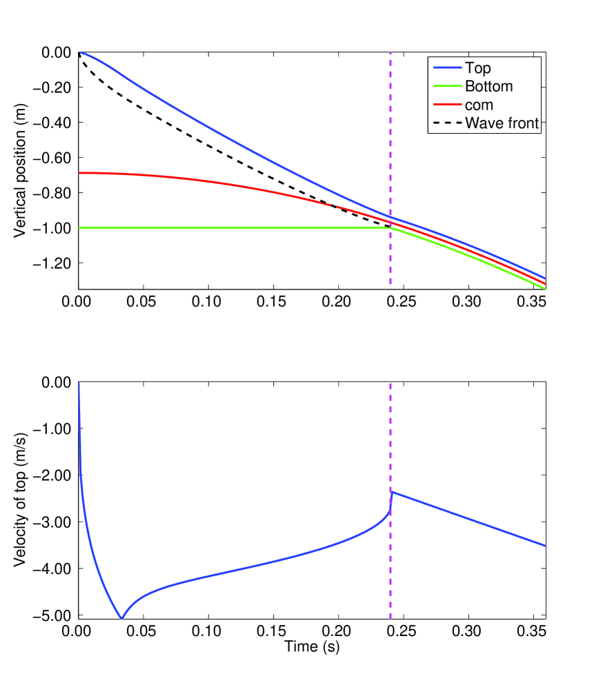
Fig. 7: The finite-collapse-time model for a falling slinky using the same slinky parameters as in Fig. 5. The collapse of the model slinky is assumed to occur via a linear decay in tension over ten turns of the slinky. Upper panel: position versus time of the slinky top (upper solid curve), center-of-mass (middle solid curve), bottom (lower solid curve), and wave front initiating collapse (dashed curve). Position is negative downwards in this figure. Lower panel: velocity of the slinky top versus time. The total collapse time $t_{c}$ is shown as the vertical dashed line in both panels.

Figure 7 shows solution of the finite-collapse time model for the typical parameters used in Figs. 4 and 5, and with a value of $\Delta$ chosen to match 10 turns of the 80-turn slinky ($\Delta=10/80=0.125$). The layout of the figure is the same as for Fig. 5. The position versus time of the top of the slinky (upper solid curve in the upper panel) is very similar to that in the instant-collapse model, but the top initially accelerates downwards from rest rather than having an initial non-zero velocity. The location of the front versus time (dashed curve in the upper panel) is significantly different to that shown in Fig. 5, and comparison of this curve and the position of the top of the slinky shows the effect of the finite time for turns to collapse behind the front. A specific feature of the motion of the front is that the initial velocity of the front is infinite (the dashed curve has a vertical slope at $t=0$). The lower panel of Fig. 7 plots the velocity versus time of the top of the slinky and shows that the top is initially at rest, then accelerates rapidly until time $t_{\mathrm{lin}}=0.03$ s during the initial linear collapse, which is marked by a sudden change in curvature of the velocity profile. The initial dynamics of the top differ from the instant-collapse model; in particular the velocity of the top of the slinky at time $t=0$ is zero, rather than having a finite value. However, after the initial acceleration of the top, the velocity variation of the top is similar to that in the instant-collapse model.

The right panel in Fig. 4 also illustrates the solution of the finite-collapse-time model with the typical parameters, showing a helix drawn to match $x(\xi,\frac{1}{2}t_{c})$—the model slinky at one half the total collapse time. The upper, dark-gray (blue online) section of the helix is the portion of the slinky above the collapse front, described by Eq. (23). The location of the collapse front is shown by a dashed horizontal line, while the dot (red online) shows the center of mass and the light-gray (green online) section at the bottom is the collapsed section in the hanging configuration.

IV Modeling real slinkies

IV.1 Data

The finite-collapse-time model from Section III.3 is compared with data obtained for two real slinkies, labeled A and B. The masses, lengths, and numbers of turns of the slinkies are listed in Table I. Slinky A is a typical metal slinky and slinky B is the light plastic rainbow-colored slinky shown in Fig. 2. These two slinkies were chosen because they have significantly different parameters.

Table 1: Measured data for two real slinkies.

	Slinky A	Slinky B
Mass $m$ (g)	215.5	48.7
Collapsed length $l_{1}$ (mm)	58	66
Stretched length $X_{\mathrm{B}}$ (m)	1.26	1.14
Number of turns $N$	86	39

The slinkies are suspended from a tripod and released, and the fall is captured with a Casio EX-F1 camera at 300 frames/s. The positions of the top and bottom of each slinky are determined from the movies at time steps of $\tau=0.01$ s in each case. Figure 2 shows frames from the movie used to obtain the data for slinky B.

IV.2 Fitting the data and model

The finite-collapse time model from Section III.3 is applied to the data for the two slinkies as follows. The observed positions for the top of each slinky during its fall are fitted to the model using least squares for all time steps. The free parameters in the model are taken to be the collapse mass fraction $\Delta$, the spring constant $k$, and an offset $t_{0}$ to time, which describes the time of release of the slinky compared to the time of the first observation. The parameter $t_{0}$ is needed because the precise time of release is difficult to determine accurately. The additional slinky parameters used are the measured values of the collapsed length $\ell_{1}$, the hanging length $X_{\mathrm{B}}$, and the mass $m$. (Given $\ell_{1}$, $X_{\mathrm{B}}$, $m$, and a chosen value of $k$, Eq. (11) determines the value of $\xi_{1}$, so equivalently, $\xi_{1}$ could be taken as a free parameter instead of $k$.)

The method of fitting is to fit the data values $x_{\mathrm{T}}(t_{n})$ for the positions of the top of a slinky ($T$ denotes top) at the observed times $t_{n}=(n-1)\tau$ (with $n=1,2,...$) to the model function for the positions evaluated at the offset time, i.e. the fit is made to $x(\xi,t)$ evaluated at $\xi=0$ and $t=t_{n}-t_{0}$. The model function $x(\xi,t)$ is defined by Eqs. (24), (25), (33), and (34) (and by the hanging configuration $X(\xi)$ for $t<t_{0}$). This procedure correctly identifies $t=t_{0}$ as the time of release.

Table II lists the best-fit parameters for the slinkies. The value of $\Delta$ is given both as a mass fraction and in terms of the corresponding number of turns of the slinky. For the plastic slinky $\xi_{1}=1$, implying that no turns are collapsed at the bottom of the slinky in the hanging configuration. Inspection of the top left frame in Fig. 2 suggests that this is correct.

Table 2: Best-fit model parameters for the slinkies.

	Slinky A	Slinky B
Spring constant $k$ (N/m)	0.69	0.22
$\xi_{1}$	0.89	1
$\xi_{1}$ (collapsed turns)	9.5	0
$\Delta$	0.045	0.45
$\Delta$ (turns)	3.9	18
$t_{0}$ (s)	0.022	0.01
Total collapse time $t_{c}$ (s)	0.27	0.27
Linear collapse time $t_{\mathrm{lin}}$ (s)	0.014	0.12

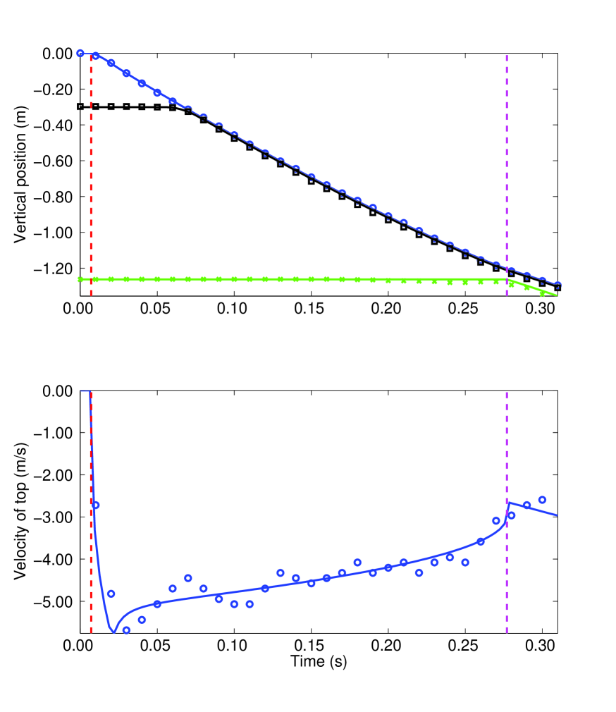
Fig. 8: The finite-collapse-time model applied to slinky A. The upper panel shows position versus time for the slinky top (upper), turn 10 (middle), and slinky bottom (lower), with the observed data represented by symbols and the best-fit model values by curves. The fitting is based on the observed positions of the slinky top. The lower panel shows the velocity of the slinky top versus time. The vertical dashed lines in both panels show the time of release of the slinky (left), which is a model parameter, and the model collapse time (right).

Figures 8 and 9 show the fits between the model and the observed data for Slinkies A and B, respectively. The upper panel in each figure shows positions versus time for the slinky top (model: upper solid curve, data: circles, blue online), turn 10 (model: middle solid curve, data: squares, black online), and the slinky bottom (model: lower solid curve, data: $\times$, green online). The lower panel in each figure shows the velocity of the top of the slinky versus time (model: solid curve, data: circles, blue online). The measured velocity of the top of the slinky is determined by centered differencing of the observed position values, i.e. the velocity at time $t_{n}$ is approximated by

$$v_{\mathrm{T}}(t_{n})=\frac{x_{\mathrm{T}}(t_{n+1})-x_{\mathrm{T}}(t_{n-1})}{2\tau}.$$ (36)

These values are estimated for illustrative comparison with the model, but they are not used in the fitting, which uses only the position data for the top shown in the upper panel. Note also that the lower panel shows downward values as negative, i.e. it shows $-v_{\mathrm{T}}(t_{n})$ versus $t_{n}$. Both panels in Figs. 8 and 9 also show the time offset $t_{0}$ for the model by the left vertical (red online) dashed line, and the total collapse time for the model by the right vertical (pink online) dashed line.

The results in Figs. 8 and 9 demonstrate that the model achieves a good qualitative fit to the observed positions of the top of each slinky. The quality of the fit is shown in the approximate reproduction of the values of the velocity of the top of each slinky obtained by differencing the position data for the top. In particular, the description of the finite time for collapse of the slinky top given by Eq. (22), with the best-fit model values, approximately reproduces the observed initial variation in the velocity of the top of each slinky shown in the lower panels of the figures. Although we do not attempt a detailed error analysis, it is useful to consider the expected size of uncertainties in the data values. If the observed position values are accurate to $\sigma_{x}\approx 0.5$ cm, the uncertainty in velocity implied by the centered differencing formula Eq. (36) is

$$\sigma_{v}=\frac{\sigma_{x}}{\sqrt{2}\tau}\approx 0.4\,\mathrm{m/s}.$$ (37)

The detailed differences between the observed and best-fit model velocity values are approximately consistent with Eq. (37).

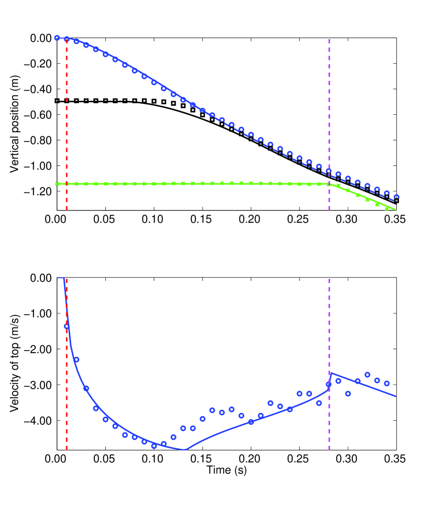
Fig. 9: The finite-collapse-time model applied to slinky B. The presentation is the same as in Fig. 8.

The fit is better for slinky A than slinky B, as shown by specific discrepancies between the model and observed data for the position of turn 10 (upper panel of Fig. 9), and the velocity of the top (lower panel of Fig. 9). This may be due to the technique used to hang the slinky: the top turns are tied together to allow the slinky to be hung vertically (see the first frame in Fig. 2). About a turn and a half of the slinky was joined at the top, and as a result the top of the slinky is heavier than in the model, and there is approximately one fewer turn. The same technique was used for both slinkies, but the effect may be more important for slinky B, which is significantly lighter and has fewer turns, than slinky A. We make no attempt to incorporate this in our model.

The best-fit values for the model parameter $\xi_{1}$ may be checked by comparison with the observed number of collapsed turns $N_{c}$ at the bottom of each slinky in the hanging configuration, which is given by Eq. (8). Alternatively, the model values for the spring constant $k$ may be checked by comparison with the period of the fundamental mode of oscillation of the slinky when it is hanging young93

$$T_{0}=4\sqrt{\frac{m}{k}}.$$ (38)

Table 3 lists the predictions for $N_{c}$ and $T_{0}$ based on the model values of $\xi_{1}$ and $k$, and the observed values for each slinky.

Table 3: Predictions (for best-fit model parameters) and observations for the number of collapsed turns when hanging, and for the fundamental mode frequency.

	Slinky A	Slinky B
Model fundamental period $T_{0}$ (s)	2.23	1.88
Observed fundamental period (s)	2.18	1.77
Model number of collapsed turns $N_{c}$	9.5	0
Observed number of collapsed turns	10	0

Table 3 shows that the slinky model with best-fit parameters approximately reproduces the observed fundamental mode periods and numbers of collapsed turns for the two slinkies. (Note that the two model values $N_{c}$ and $T_{0}$ are not independent.) The discrepancies between the model and observed values for the fundamental periods are $\sim 5$%, with the model values being too large in both cases. It is useful to consider the expected size of discrepancies in the period produced by observational uncertainties. From Eqs. (11), (18), and (38) it follows that

$$t_{c}=\frac{4}{3}\left[\frac{2(X_{\mathrm{B}}-\ell_{1})}{g}\right]^{3/4}\frac{1}{\sqrt{T_{0}}}.$$ (39)

Assuming the distances $X_{\mathrm{B}}$ and $\ell_{1}$ are well-determined, Eq. (39) implies

$$\frac{\sigma_{T_{0}}}{T_{0}}=2\frac{\sigma_{t_{c}}}{t_{c}},$$ (40)

where $\sigma_{T_{0}}$ and $\sigma_{t_{c}}$ are the uncertainties in $T_{0}$ and $t_{c}$ respectively. Taking the value of the time step $\tau=0.01$ s as a representative value for $\sigma_{t_{c}}$ in Eq. (40) gives $\sigma_{T_{0}}/T_{0}=0.08$, i.e. an 8% error in the model value for the fundamental mode period. This suggests that the model values for $T_{0}$ are as accurate as might be expected from observational uncertainties, and indicates that it is difficult to determine the mode period for a real slinky based on measuring the fall of the slinky.

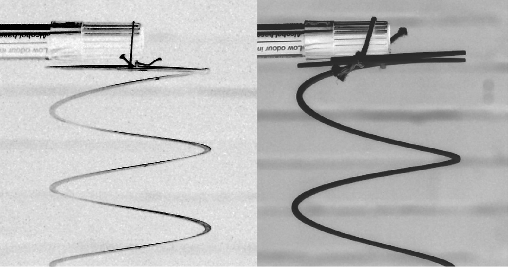
Fig. 10: An experiment with different methods of suspension of the top of slinky B. In the left-hand image the top is suspended from a string tied across a diameter of the first turn of the slinky. In the right-hand image the string is tied around the first two turns.

The technique of suspension of the top of the slinky, involving tying about a turn and a half of the slinky together to ensure that it hangs vertically, introduces some uncertainty into the modeling. It is interesting to investigate the effect of this step on the initial dynamics of the slinky during the fall. For this purpose the slinky is suspended in two additional ways, with a string tied across both sides of just the top turn, and with a string tied across both sides of the top two turns, linked together. These methods of suspension involve fewer, and greater numbers of turns tied together at the top, respectively, compared with the original method (which had about a turn and a half tied together at the top). Figure 10 illustrates the two methods of suspension, showing images (in inverted grayscale for clarity) of the top few turns of the slinky in the two cases. The left-hand image shows the case with one turn tied together at the top while the right-hand image shows the case with two turns tied together.

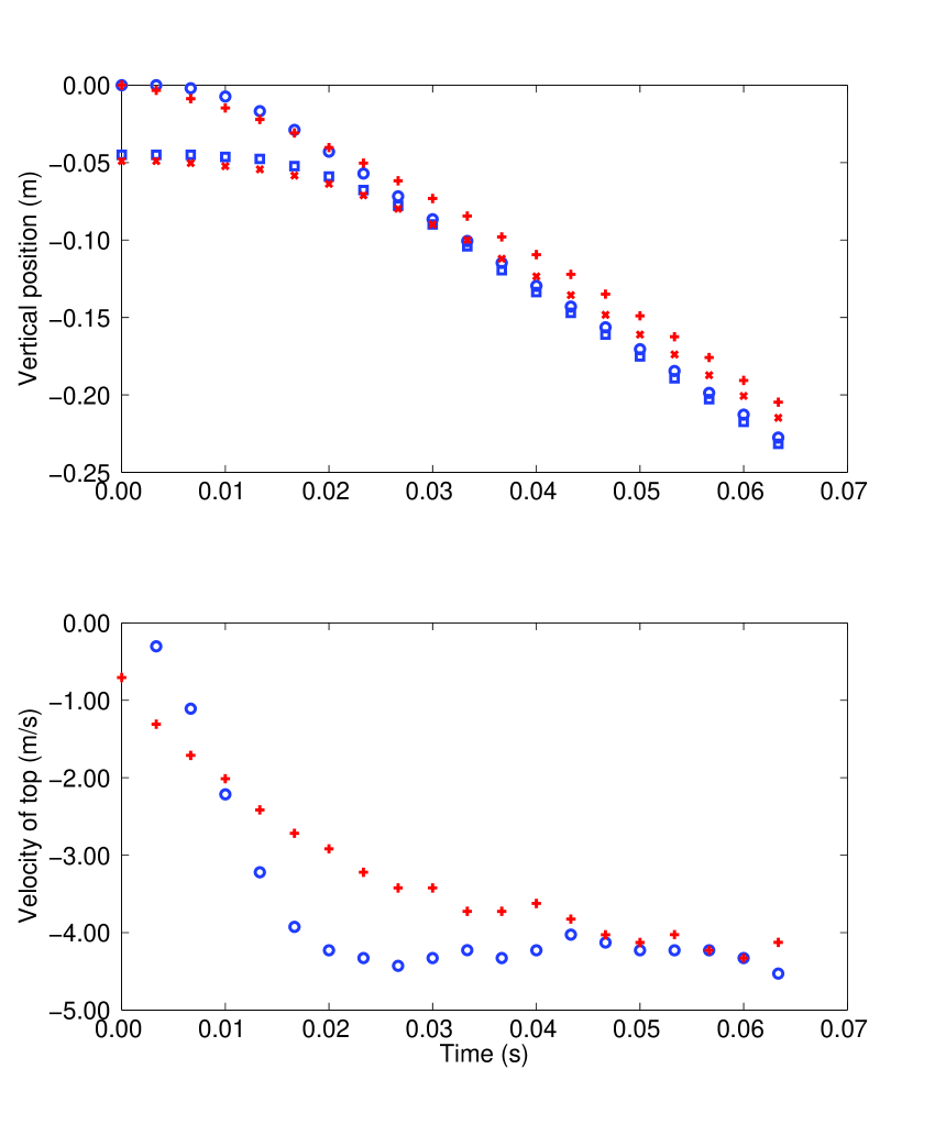
Fig. 11: Data extracted for the initial fall of slinky B following suspension using the two methods shown in Fig. 10. The circles and squares show results for suspension by one turn and the $+$ and $\times$ symbols for suspension by two turns. The upper panel shows the position versus time of the top and of the first turn below the initially tied top section. The lower panel shows the velocities of the top in each case, obtained by differencing the position data (circles for suspension by one turn and $+$ symbols for suspension by two).

With these methods of suspension the slinky is filmed being dropped, and data are extracted for the first 0.06 s of the fall in each case; the results are shown in Fig. 11. The upper panel shows the positions versus time for the top of the slinky and for the first turn below the turns tied at the top, for each case: circles and squares, respectively for suspension by one turn, and $+$ and $\times$ symbols, respectively for suspension by two. The lower panel shows the velocities of the top in each case, obtained by differencing the position data using Eq. (36) (circles for suspension by one turn and $+$ symbols for suspension by two). These results show that the top of the slinky accelerates from rest more rapidly when fewer turns are tied together at the top, which is expected because the inertia of the top is reduced. However, in both cases the top achieves a very similar velocity after $\sim 0.05$ s. It is expected that the subsequent dynamics of the collapse of turns will be similar in the two cases. The dependence of the initial dynamics of the top on the method of suspension will influence the estimates of model parameters, in particular the collapse mass fraction $\Delta$. However, it is expected that the estimate of the spring constant $k$ will be less influenced because this parameter is determined largely by the identification from the data of the total collapse time $t_{c}$. The dependence of the fitting on the method of suspension of the top of the slinky could perhaps be reduced by fitting to the positions of turns other than the top turn during the fall.

V Conclusions

The fall of a slinky illustrates the physics of a tension spring, and more generally wave propagation in a spring. This paper investigates the dynamics of an initially stretched slinky that is dropped. During the fall the slinky turns collapse from the top down as a wave front propagates along the slinky. The bottom of the slinky does not begin to fall until the top collides with it. A modification to an existing model calkin93 for the fall is presented, providing an improved description of the collapse of the slinky turns. The modification is the inclusion of a finite time for collapse of turns behind the downward propagating wave front. The new model is fitted to data obtained from videos of the falls of two real slinkies having different properties.

The model is shown to account for the observed positions of the top of each slinky in the experiments, and in particular reproduces the initial time-profile for the velocity of the top after release. The spring constant of the slinky is assumed as a free parameter in the model, and the best-fit model values are tested by comparison with independent determinations of the fundamental mode periods for the two slinkies, which depend on the spring constants. The model values appear consistent with the observations taking into account the observational uncertainties.

The new model for the slinky dynamics during the fall developed here is semi-analytic, and allows treatment of a tension spring including approximate description of the dynamics of the collapse of the spring. During the collapse of the top of the slinky the turns collide, but the model does not describe this process in detail. Instead, the collapse is approximately described by the assumption of a linear decrease in tension as a function of mass density along the spring behind the front initiating the collapse. The linear approximation is motivated by the experimental data from the slinky videos, which shows that the spacing between slinky turns during the collapse decreases approximately linearly with time.

The behavior of a falling slinky is likely to be counter-intuitive to students and provides a useful (and very simple) undergraduate physics lecture demonstration. The explanation of the behavior may be supplemented by showing high-speed videos of the fall. The modeling of the process presented here is also relatively simple, and should be accessible to undergraduate students.

Fig. 2: Frames extracted from a high-speed video of the fall of a rainbow-colored slinky, illustrating the collapse of the top of the slinky, and the continued suspension of the bottom after release of the top. The top end of the slinky takes $\sim 0.25$ s to reach the bottom.

References

- (1) S. Y. Mak, “The static effective mass of a slinkyTM,” Am. J. Phys. 61, 261–264 (1993).
- (2) M. Sawicki, “Static elongation of a suspended slinkyTM,” Phys. Teacher 40, 276–278 (2002).
- (3) A.-P. Hu, “A simple model of a Slinky walking down stairs,” Am. J. Phys. 78, 35–39 (2010).
- (4) J. M. Bowen, “Slinky oscillations and the notion of effective mass,” Am. J. Phys. 50, 1145–1148 (1982).
- (5) R. A. Young, “Longitudinal standing waves on a vertically suspended slinky,” Am. J. Phys. 61, 353–360 (1993). Young’s expressions for mode periods and frequencies refer to the mass per turn , and spring constant per turn , of the slinky. These are related to the values for the whole slinky, used in this paper, by and , respectively.
- (6) J. Blake and L. N. Smith, “The Slinky® as a model for transverse waves in a tenuous plasma,” Am. J. Phys. 47, 807–808 (1979).
- (7) F. S. Crawford, “Slinky whistlers,” Am. J. Phys. 55, 130–134 (1987).
- (8) G. Vandegrift, T. Baker, J. DiGrazio, A. Dohne, A. Flori, R. Loomis, C. Steel, and D. Velat, “Wave cutoff in a suspended slinky,” Am. J. Phys. 57, 949–951 (1989).
- (9) M. G. Calkin, “Motion of a falling spring,” Am. J. Phys. 61, 261–264 (1993).
- (10) J. M. Aguirregabiria, A. Hernandez, and M. Rivas, “Falling elastic bars and springs,” Am. J. Phys. 78, 583–587 (2007).
- (11) W. G. Unruh, “The Falling slinky,” arXiv:1110.4368v1 (19 Oct 2011): <http://arxiv.org/abs/1110.4368>.
- (12) The high-speed videos used to obtain data in this paper are available (as reduced, compressed versions) as supplementary material from [AIP to insert URL] and also at <http://www.physics.usyd.edu.au/~wheat/slinky/>. Also provided are animations of the solutions to the instant-collapse and finite-collapse-time model, and an animation of the fundamental mode of oscillation of the hanging slinky.
- (13) The YouTube video is at <http://www.youtube.com/watch?v=eCMmmEEyOO0>.
- (14) T. W. Edwards and R. A. Hultsch, “Mass distribution and frequencies of a vertical spring,” Am. J. Phys. 40, 445–449 (1972).