A Temporal Map in Geostationary Orbit: The Cover Etching on the EchoStar XVI Artifact

Abstract

Geostationary satellites are unique among orbital spacecraft in that they experience no appreciable atmospheric drag. After concluding their respective missions, geostationary spacecraft remain in orbit virtually in perpetuity. As such, they represent some of human civilization’s longest lasting artifacts.

With this in mind, the EchoStar XVI satellite, to be launched in fall 2012, will play host to a time capsule intended as a message for the deep future. Inspired in part by the Pioneer Plaque and Voyager Golden Records, the EchoStar XVI Artifact is a pair of gold-plated aluminum jackets housing a small silicon disc containing one hundred photographs. The Cover Etching, the subject of this paper, is etched onto one of the two jackets. It is a temporal map consisting of a star chart, pulsar timings, and other information describing the epoch from which EchoStar XVI came. The pulsar sample consists of 13 rapidly rotating objects, 5 of which are especially stable, having spin periods $<10$ ms and extremely small spindown rates.

In this paper, we discuss our approach to the time map etched onto the cover and the scientific data shown on it; and we speculate on the uses that future scientists may have for its data. The other portions of the EchoStar XVI Artifact will be discussed elsewhere.

1. Introduction

In the early 1970s, a group of scientists and artists led by Carl Sagan and Frank Drake designed several artifacts and messages intended for extraterrestrial audiences. The first was the Pioneer Plaque placed on the Pioneer 10 and 11 spacecraft, launched in 1972 and 1973, respectively (Sagan et al 1972). In 1974, Frank Drake composed the “Arecibo Message,” a 1679-bit digital transmission beamed toward star cluster M13 to celebrate the renovation of the Arecibo Observatory. More detailed messages, including images and sounds, were encoded onto the phonographic Golden Records and placed on the Voyager 1 and 2 spacecraft, launched in 1977 toward deep space (Sagan et al 1978).

While geostationary spacecraft do not leave the solar system or even the Earth’s environs, they inhabit time in a way that is similar to deep space probes. Located in the so-called “Clarke Belt,” some 36,000 km above the equator, geostationary communications satellites experience no appreciable atmospheric drag. These spacecraft have one of two fates. International regulations stipulate that satellite operators conduct end-of-life maneuvers to place derelict satellites into supersynchronous “graveyard” orbits (Collis 2009). In practice, however, operators regularly leave their spent satellites in loosely geosynchronous orbits. In both cases, these spacecraft remain orbiting virtually in perpetuity (Walker & King-Hele 1986; Flohrer et al 2011). As such, geostationary satellites are undoubtedly some of contemporary civilization’s longest-lasting objects. As a scientific and cultural exercise, we can imagine scientists in the distant future looking in this zone for relics from past civilizations (Freitas & Valdes 1983, 1985). The EchoStar XVI Artifact represents an effort to communicate with these future scientists.

The full Artifact is composed of two interlocking gold-plated aluminum jackets housing a silicon disc called “The Last Pictures,” on which 100 photographs are nano-etched. The Artifact Cover Etching is located on the exterior of one of the two jackets.

In this paper, we focus on the Artifact Cover Etching, wherein we endeavored to create a map explaining when the spacecraft originated, to whomever may find it in the future. Specifically, we detail the several scientific and mathematical messages we developed for the Artifact Cover. The photographic contents of the Artifact’s silicon disc are detailed elsewhere (Paglen 2012).

2. Artifact Cover Theory and Design

Some of the basic ideas that informed our time-map were developed by Sagan et al (1972, 1978) for the Pioneer and Voyager missions, which we took as a starting point. Scientific developments since the 1970s have provided some interesting new possibilities described below. Another essential difference between this and earlier plaques is that ours is locked in perpetual Earth orbit, and therefore obviously associated with our planet. Consequently, we made no effort to communicate the Artifact’s place of origin. Instead, our temporal map seeks to indicate the spacecraft’s Epoch of Origin using currently measured quantities such as the South Celestial Pole location, Earth’s stellar rotation period, location of tectonic plates, orbital period of the Moon, locations of stars and extragalactic radio sources, and positions and periods of pulsars. The map, as etched onto the Artifact Cover, is shown in Fig. 1, and its various elements are discussed below.

2.1. Fundamental Unit of Frequency, Time, and Epoch of Origin

We use the hyperfine ground-state transition of neutral atomic hydrogen as the fundamental unit of frequency $f_{0}$ and time $t_{0}=1/f_{0}$ on the Artifact Cover. This transition is illustrated by a sketch of neutral atomic hydrogen in each of the two possible hyperfine states (see Fig. 1). The sketch is identical to the one on the Pioneer Plaques, which used the same transition as their fundamental temporal unit (Sagan et al 1972). Although the International Committee for Weights and Measurements pegs the duration of one second to the ground-state cesium-133 hyperfine transition (Conference Generale des Poids et Mesures 1968), we chose to continue using the hydrogen transition both as a nod to the work of Sagan et al (1972), in addition to the following practical reasons: Hydrogen is the most abundant element in the universe; and, as the simplest element, it is far easier to sketch than cesium. Equally important, the currently accepted value of the hydrogen hyperfine transition, with $f_{0}=(1,420,405,751.768\pm 0.001)$ s^-1 (Kramida 2010), is adequately defined and sufficiently accurate and precise for our purposes.

The Epoch of Origin is nominally 2011 Oct 4.0 UT (MJD 55838.0). However, some of the items on the Artifact Cover were plotted using a slightly different epoch for ease of calculation, if the results are not noticeably affected. The actual epochs are given below.

2.2. Fundamental Spatial Reference System

The Artifact Cover requires a spatial reference system against which to measure various quantities. A plot of the locations of the brighter stars and pulsars (see §2.3.4) centered on the South Celestial Pole (SCP), with the current location of the SCP also marked, serves adequately on a timescale of $\lesssim 10^{3}$ yr. On longer timescales, the SCP and many of the stars and pulsars will move in various directions across the sky, rendering their patterns on the Artifact Cover increasingly hard to decipher. (See §2.3.1 for discussion of the future motions of the SCP.)

Consequently, we require longer-lived, relatively fixed objects or phenomena to delineate the reference frame on the longest timescales. Therefore we also plotted the brightest point-like radio sources (NRAO 2011). These objects, mostly Active Galactic Nuclei (AGN) in deep space, will exhibit very small angular motions over cosmic timescales, although their intense radio emissions will fade within $10^{7-8}$ yr (Porciani et al 2004).

2.3. Epoch of Origin Markers

In this subsection, we detail each of the Epoch of Origin markers located on the Artifact Cover. As we shall later show, the redundant nature of the information on these Markers enables them to be used for other purposes as well.

2.3.1 Terrestrial Spin Axis Precession

The precession of the Earth’s spin axis provides one means of identifying the Epoch of Origin of this Artifact. The intersection of the two lines crossing the sky map in Fig. 1 marks the current location of the SCP. Note however that the approximately cyclical nature of the precession (with $23\fdg 3\pm 1\fdg 3$ obliquity) brings the SCP close to this location at $\sim 26$-kyr intervals, rendering precession unusable as an Epoch of Origin Marker on timescales of this order or longer. On very long timescales, however, Earth’s spin axis obliquity may undergo major chaotic changes due to solar system resonances (Tomasella et al 1996, Neron de Surgy & Laskar 1997), at which time the marked location and hence the obliquity of today’s pole would again serve as an Epoch of Origin marker, albeit crude.

2.3.2 The Earth’s Stellar Day and the Moon’s Sidereal Month

According to Lunar Laser Ranging, our Moon’s orbital radius is expanding by 38 mm/yr (Chapront et al 2002), at the expense of a lengthening of the Earth’s spin period. Hence, by specifying on Fig. 1 the Earth’s stellar rotation period to be 86,164.101 s, and the Moon’s sidereal orbital period [1 sidereal month = 27.321661 mean solar days = 27.396462 stellar days (Kay & Laby 1995) ], we implicitly specify the epoch at which these constantly-changing quantities were measured (approximately 1990 CE)

2.3.3 Tectonic Plate Motions

The map of the Earth itself provides a much cruder estimate of the Epoch of Origin of the Artifact, since motion of the tectonic plates will slowly distort the shape and location of the continents over time.

2.3.4 Millisecond Pulsars

By far the most precise Epoch of Origin markers are provided by the inscribed pulse periods of millisecond pulsars (MSPs). Since all pulsars’ intrinsic spin periods are lengthening with time, the choice of a particular value of the period specifies the epoch at which it was determined. Pulsars, having been discovered only a few years before the Pioneer launches (Hewish et al 1968), were also used as Epoch (and Location) of Origin Markers on those spacecraft plaques. However, although the pulsars known at that time were remarkably stable clocks, they can not compare with the stunning stability (Shannon & Cordes 2010, Hartnett & Luiten 2011) of the subsequently discovered (Backer et al 1982) MSPs. We determined $P(T)$, the MSP period at our Epoch of Origin $T$, using its measured period $P_{0}$ at a given epoch $T_{0}$, and period derivative or “spindown rate” $\dot{P}$ (Manchester et al 2005):

$$P(T)=P_{0}+\dot{P}(T-T_{0}).$$ (1)

The period uncertainty $\Delta P$ and Epoch of Origin uncertainty $\Delta T$ were calculated by propagating the uncertainties (Manchester et al 2005) in the quantities used in Eq. 1:

$$\Delta T=\frac{\Delta P(T)}{\dot{P}}=\frac{\sqrt{[\Delta P_{0}]^{2}+[\Delta\dot{P}(T-T_{0})]^{2}}}{\dot{P}}.$$ (2)

While normal pulsars are thought to stop shining after $10^{6-7}$ yr, MSPs, which have been spun up by accretion of matter from a companion, appear to have much longer radio-emitting lifetimes (possibly comparable to the age of the universe). Table 1 and Fig. 1 give the locations and periods of 13 MSPs at Epoch of Origin $T=$ 2011 Oct 4.0. (Figure 1 gives the pulsar periods in units of $t_{0}$, using base-2 numbers.) The Table also lists $\Delta T$, the remarkably small uncertainty in $T$, calculated via Eq. 2. The final set of 13 MSPs was winnowed from the list of all pulsars in the ATNF catalogue (Manchester et al 2005) as follows: First, we eliminated pulsars with periods $P>0.100$ s. All pulsars in globular clusters were also eliminated because their circumcluster orbits lead to complicated, temporally-varying changes in their apparent periods. Next, we removed those with measured angular velocities across the sky, since such motions, if measurable, are also large enough to render the objects invisible or unidentifiable on long timescales. Then, short orbital-period binary pulsars were eliminated because radio beams may precess away from Earth due to the pulsars’ relativistic interactions with the companion (Weisberg & Taylor 2002), or to pulsars’ demise because of gravitational radiation-induced orbital decay (Weisberg et al 2010) and coalescence. Some of the final 13 MSPs as selected above are actually young pulsars with rather large spindown rates and short lifetimes. The periods that are written on the Cover Etching are truncated just beyond the last significant (base-2) digit as indicated by Eq. 2, in accord with standard scientific practice. Additional MSPs, though meeting the above criteria, are plotted without written periods simply because the string of binary digits would not fit comfortably on the Artifact Cover.

3. Future Fate of the Artifact and its Cover

At the end of its active life approximately 15 years after launch, EchoStar XVI is scheduled to boost into a slightly higher “graveyard” orbit in order to free up valuable space in the geostationary zone. Interestingly, as the Earth’s spin gradually slows, the altitude of the geostationary zone will migrate outwards, eventually to coincide with today’s graveyard. The spacecraft and its Artifact should orbit indefinitely in the graveyard, since its altitude places it well above the last wisps of atmosphere. They will occasionally encounter space debris (both natural and human-made) in this zone, but the Artifact’s hardened nature should shield it from all but the most extreme collisions. According to recent modeling (Schröder & Connon Smith 2008), the Sun’s luminosity will slowly increase over the next 5 billion yr to almost double its current value, thereby also doubling the solar flux delivered to the Artifact, which is designed easily to survive the enhanced flux. At around the same time, fusion in the Sun’s core will cease due to hydrogen depletion, and over the next 2 billion years its outer layers will expand approximately to the radius of the Earth’s orbit, thereby enveloping (or nearly so) our planet and its surroundings. (Earth’s orbit will also migrate outwards as the Sun loses significant mass due to winds at these late stages, which may prevent our direct immersion.) At that time, the Sun will also radiate almost three thousand times its current luminosity. The Artifact, even if it has survived to this point, will likely not outlive these events.

4. Discussion

A comparison of the messages and the technologies on the current Artifact with those on the Pioneer and Voyager spacecraft indicates the rapid pace of technological advance over even just a few decades. While we have endeavored to use putatively universal symbols, the question of whether our temporal map would be decipherable by deep-future humans or extra-terrestrial spacefaring civilizations is a deeply controversial one that intersects fields from philosophy of science to anthropology, semiotics, and cognitive science. As such, the question of its future intelligibility is outside the scope of our discussion here. To illustrate how future scientists and archaeologists may use the data provided in our time-map, however, we will assume that it will be intelligible by any spacefaring civilization; i.e., any civilization with the means to examine it.

4.1. Determining the Time Elapsed between Origin and Discovery

Our Etching’s temporal map contains a mixture of “clocks,” some of which are expected to run at constant rates over cosmological times (e.g., the hydrogen hyperfine transition frequency), while others’ rates will vary (e.g., the Earth’s spin period). Depending on the level of their scientific knowledge, the discoverers may be able to determine the Epoch of Origin of the Artifact by comparing Epoch of Origin clock rates with Epoch of Discovery clock rates. For example, they could measure at the Epoch of Discovery, the periods $P$ and spindown rates $\dot{P}$ of some of the 13 MSPs whose Epoch of Origin periods are written on the etching. Then they could use Eq. 1 to determine $(T-T_{0}),$ the time elapsed between the two epochs.

If the elapsed time is sufficiently long, higher derivatives must be added to Eq. 1. While current pulsar theory gives an expected value of the next derivative $\ddot{P}$ under the assumption of rotational energy loss to magnetic dipole radiation (Lyne & Graham-Smith 2012, p. 72),

$$\ddot{P}=-\frac{\dot{P}^{2}}{P},$$ (3)

this expression has been shown to be a poor approximation to reality in the few cases where the next derivative has actually been measured (Gradari et al 2011). Similar arguments apply to the other clocks such as the Earth’s spin period and the Moon’s orbital period. Nevertheless, the discoverers should be able to ascertain the true elapsed time by checking the consistency of their multiple results from an ensemble of such “clocks.”

4.2. Testing and Refining Scientific Theories

Once the discoverers establish $(T-T_{0}),$ the time elapsed since the origin of the Artifact, they will also have the opportunity to test and refine some of their scientific theories over deep time. For example, they could combine our inscribed data with their measurements, thereby directly determining higher order derivatives as discussed above. The assumptions underlying the theories could then be tested via comparison of these measured higher derivatives with the theoretically predicted ones, as shown in the above pulsar spindown example.

Some of our current clocks may “break” over cosmic timescales, in which case the discoverers will derive totally unique information by decoding our measurements. For example, the pacing of resonances causing major changes in our spin axis obliquity is dictated by changes in tidal dissipation in the Earth-Moon system, which is dependent on tectonic plate motions and other geophysical processes whose details are poorly known over long timescales, but which could be constrained by data from our era.

The discoverers might further be able to apply our currently recorded measurements for uses that we cannot foresee, much as we now use ancient solar eclipse records to provide unique data on the evolution of the Earth’s spin period over historic times (Stephenson 1997). In addition, the mere discovery of the Artifact and spacecraft in geostationary space could provide the discoverers with a wealth of information on us, much as the discovery of the “Antikythera Mechanism” astronomical computer (Freeth et al 2006) in a shipwreck has done for our knowledge of ancient Mediterranean scientific and technological expertise. Further, we can hope that any collisions suffered by the Artifact before its discovery will not prevent its decoding, much as erosion of the Antikythera Mechanism slowed but did not stop current researchers from deciphering much of it.

Table 1Table 1: Parameters of the millisecond pulsars whose periods are inscribed on the Cover Etching.

Pulsar Name	Period $P$ at $T=$	$\dot{P}$	$\Delta T$
	2011 Oct 4.0 UT (s)	s/s	(d)
J1016-5819	0.0878344385(2)	$6.980(4)\times 10^{-16}$	2.7
J1629-6902	0.0060006034468(1)	$1.00(3)\times 10^{-20}$	127
J1454-5846	0 .045248773318(4)	$8.17(9)\times 10^{-19}$	50
J1435-6100	0.0093479722199(2)	$2.45(5)\times 10^{-20}$	93
J1420-6048	0.068210329(1)	$8.3167(3)\times 10^{-14}$	0.15
J1232-6501	0.08828190855(1)	$8.1(3)\times 10^{-19}$	169
J1216-6410	0.00353937565876(4)	$1.6(2)\times 10^{-21}$	288
J1125-6014	0.00263038074072(2)	$4.01(9)\times 10^{-21}$	61
J1112-6103	0.0649748526(5)	$3.1460(1)\times 10^{-14}$	0.2
J1055-6028	0.09966459910(6	$2.95322(5)\times 10^{-14}$	0.03
J1103-5403	0.00339270965950(6)	$3.7(10)\times 10^{-21}$	192
J0940-5428	0.0875586849(4)	$3.2868(1)\times 10^{-14}$	0.14
J0855-4644	0.06468893573(1)	$7.26269(3)\times 10^{-15}$	0.02

Note. — Uncertainties in the last digit(s) of measured quantities are given in parentheses..

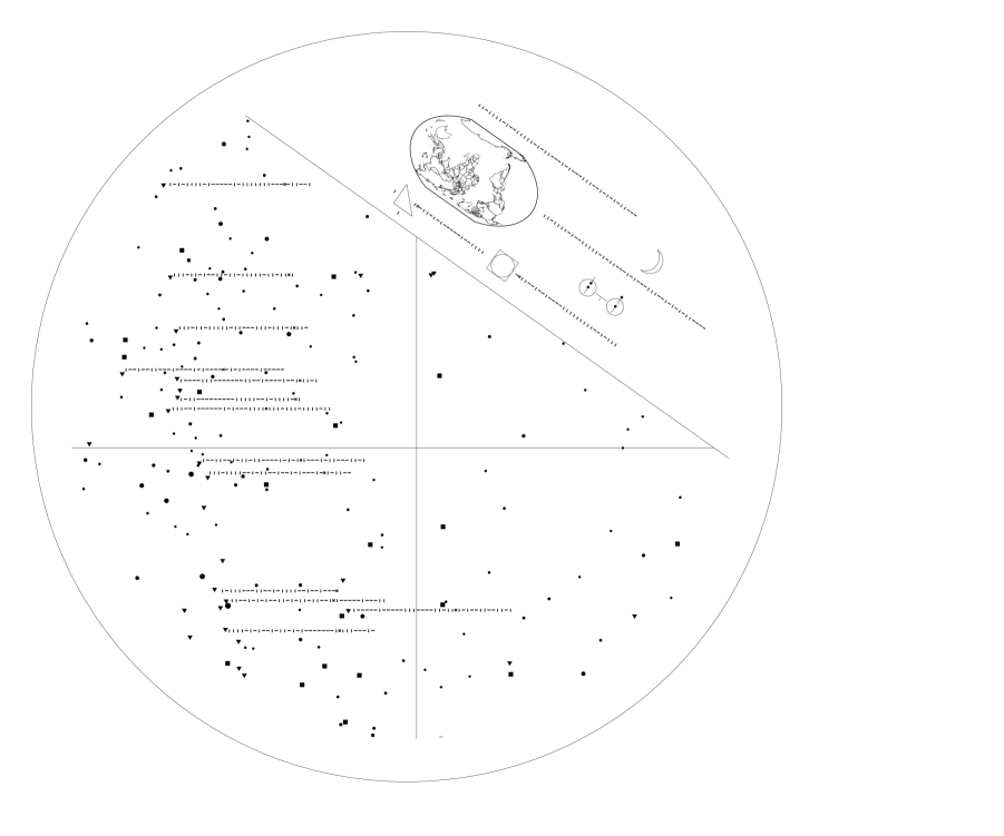
Figure 1.— The Cover Etching portion of the Artifact, to be launched on the exterior of the EchoStar XVI satellite. The image is dominated by a map of the southern sky. Stars are denoted by circles whose size is proportional to their apparent brightness at visual wavelengths. Point radio sources, mostly Active Galactic Nuclei, are represented by squares. Millisecond pulsars are symbolized by triangles; some of whose periods on Epoch of Origin Date 2011 Oct 4.0 UT are given in base-2 numbers, which utilize only zeros (“-”) and ones (“$|$”),and a placeholder (“$\times$”) to distinguish the whole and fractional parts. The two lines crossing the whole skymap denote RA = (0, 90, 180, and 270)$\arcdeg$, and their crossing point marks the South Celestial Pole at Epoch 2000.0 CE. Also shown are the current arrangement of continents on the Earth, the rotation period of the Earth and the revolution period of the Moon. All time intervals are given in units of the period of the ground-state hyperfine transition of atomic hydrogen, except for the lunar sidereal orbital period, which is denoted in units of the stellar day so as to avoid the need for 29 trailing zeros. Practice with our binary number system is given by presenting two values next to geometrical objects: the ratio of the hypotenuse and the side of a (displayed) $45\arcdeg$ right triangle; and the ratio of the areas of a circle to its circumscribed square (also displayed).

References

- Chapront et al. (2002) Chapront, J., Chapront-Touzé, M., & Francou, G. 2002, A&A, 387, 700
- Cocconi & Morrison (1959) Cocconi, G., & Morrison, P. 1959, Nature, 184, 844
-
Conference Generale des Poids et Mesures (1968)
Conference
Generale des Poids et Mesures. 1968, (13th Meeting, 1967/68, Resolution 1),
Metrologia, 4, 43, online at
http://www.bipm.org/en/CGPM/db/13/1/ - Flohrer et al (2011) Flohrer, T., Choc, R., & Bastida, B. 2011, Classification of Geosynchronous Objects, No. 13, Document GEN-DB-LOG-00074-OPS-GR, (Darmstadt, Germany: ESA ESOC)
- Freeth et al. (2006) Freeth, T., Bitsakis, Y., Moussas, X., Seiradakis, J. H., Tselikas, A., Mangou, H., Zafeiropoulou, M., Hadland, R., Bate, D., Ramsey, A., Allen, M., Crawley, A., Hockley, P., Malzbender, T., Gelb, D., Ambrisco, W., Edmunds, M. G. 2006, Nature, 444, 587
- Freitas & Valdes (1983) Freitas, R. A., Jr., & Valdes, F. 1983, Icarus, 53, 453
- Freitas & Valdes (1985) Freitas, R. A., Jr., & Valdes, F. 1985, Acta Astronautica, 12, 1027
- Gradari et al. (2011) Gradari, S., Barbieri, M., Barbieri, C., et al. 2011, MNRAS, 412, 2689
-
Groten (1999)
Groten, E. 1999, Current (1999) Best Estimates of the Parameters of
Common Relevance to Astronomy, Geodesy, and Geodynamics, (Copenhagen, Denmark:
Internat. Assoc.
Geodesy), online at
http://www.gfy.ku.dk/~iag/HB2000/part4/groten.htm. See also Internat. Earth Rot. Service, Earth Orientation Center, Useful Constants Updated March 29, 2010, (Paris, France: Observatoire de Paris), online athttp://hpiers.obspm.fr/eop-pc/models/constants.html - Hartnett & Luiten (2011) Harnett, J. G. , & Luiten, A. N. 2011, Rev. Mod. Phys., 83, 1
-
Kay & Laby (1995)
Kay, G. W. C., Laby, T. H. 1995, Tables of
Physical and Chemical
Constants, 16th ed., Sec 2.7.2, “Astronomical Units and Constants,” UK: Nat. Phys. Lab.,
online at
http://www.kayelaby.npl.co.uk/general_physics/2_7/2_7_2.html - Hewish et al. (1968) Hewish, A., Bell, S. J., Pilkington, J. D. H., Scott, P. F., & Collins, R. A. 1968, Nature, 217, 709
- Kramida (2010) Kramida, A., 2010, Atomic Data and Nuclear Data Tables 96, 586
- Lyne & Graham-Smith (2006) Lyne, A. G., & Graham-Smith, F. 2012, Pulsar Astronomy, 4th ed., Cambridge Astrophysics Series, 48. Cambridge, UK: Cambridge U. Press
-
Manchester et al. (2005)
Manchester, R. N.,
Hobbs, G. B., Teoh, A., & Hobbs, M. 2005, AJ, 129, 1993. A regularly updated version is online
at
http://www.atnf.csiro.au/research/pulsar/psrcat/. - Neron de Surgy & Laskar (1997) Neron de Surgy, O., & Laskar, J. 1997, A&A, 318, 975
-
NRAO (2011)
NRAO, 2011, Very Long Baseline Array (VLBA) Calibrator Source
List, Socorro, NM: Nat. Radio Astron. Observ., online at
http://www.vlba.nrao.edu/astro/calib/vlbaCalib.txt - Paglen (2012) Paglen, T. 2012, The Last Pictures, Berkeley: U. California Press
- Porciani et al. (2004) Porciani, C., Magliocchetti, M., & Norberg, P. 2004, MNRAS, 355, 1010
- Sagan et al. (1972) Sagan, C., Salzman Sagan, L., & Drake, F. 1972, Science, 175, 881
- Sagan et al. (1978) Sagan, C., Drake, F. D., Druyan, A., Ferris, T., Lomberg, J., Salzman Sagan, L. 1978, Murmurs of Earth: The Voyager Interstellar Record, New York, NY: Random House
- Schröder & Connon Smith (2008) Schröder, K.-P., & Connon Smith, R. 2008, MNRAS, 386, 155
- Shannon & Cordes (2010) Shannon, R. M., & Cordes, J. M. 2010, ApJ, 725, 1607
- Stephenson (1997) Stephenson, F. R. 1997, Historical Eclipses and Earth’s Rotation, Cambridge, UK: Cambridge University Press
- Tomasella et al. (1996) Tomasella, L., Marzari, F., & Vanzani, V. 1996, Planet. Space Sci., 44, 427
- Walker & King-Hele (1986) Walker, D. M. C., & King-Hele, D. G. 1986, ESA Special Publication, 246, Proc. Euro. Space Agency Workshop on Reentry of Space Debris, 29, Darmstadt, Germany: ESA SP
- Weisberg & Taylor (2002) Weisberg, J. M., & Taylor, J. H. 2002, ApJ, 576, 942
- Weisberg et al. (2010) Weisberg, J. M., Nice, D. J., & Taylor, J. H. 2010, ApJ, 722, 1030