Deconfined-critical behavior of the VBS- and nematic-order parameters for the spatially anisotropic $S=1$-spin model

Abstract

The phase transition between the valence-bond-solid (VBS) and nematic phases, the so-called deconfined criticality, was investigated for the quantum $S=1$-spin model on the spatially anisotropic triangular lattice with the biquadratic interaction by means of the numerical diagonalization method. We calculated both VBS- and nematic-order parameters, aiming to clarify the nature of this transition from complementary viewpoints. Simulating the clusters with $N\leq 20$ spins, we estimate the correlation-length critical exponent as $\nu=0.95(14)$. We also calculated Fisher’s exponent (anomalous dimension) for each order parameter.

1 Introduction

According to the deconfined-criticality scenario [1, 2, 3], in two dimensions, the phase transition separating the valence-bond-solid (VBS) and antiferromagnetic phases is continuous. (Naively [2], such a transition should be discontinuous, because the adjacent phases possess distinctive order parameters such as the VBS-coverage pattern and the sublattice magnetization, respectively.) Extensive computer simulations have been made to support this claim [4, 5]. However, still, one cannot exclude a possibility of a weak-first-order transition accompanied with an appreciable latent-heat release [6, 7, 8, 9, 10, 11, 12, 13, 14].

The magnetic frustration is a good clue to the realization of the VBS phase [14, 15, 16]. Alternatively, one is able to stabilize the VBS state with the spatial anisotropy and the biquadratic interaction [17, 18]. In our preceding paper [19], we investigated the quantum $S=1$-spin model on the spatially anisotropic triangular lattice with the biquadratic interaction, Eq. (1), and analyzed the singularity of the VBS-nematic phase transition; a schematic phase diagram is presented in Fig. 1, where the parameters $J$ and $j$ control the spatial anisotropy and the biquadratic interaction, respectively. Scrutinizing the scaling behavior of the excitation gap, we obtained the correlation-length critical exponent $\nu=0.92(10)$ [19]. In this paper, we calculate both VBS- and nematic-order parameters, and survey the criticality from complementary viewpoints.

To be specific, we present the Hamiltonian for the $S=1$-spin model on the spatially anisotropic triangular lattice with the biquadratic interaction

$${\cal H}=-J\sum_{\langle ij\rangle}[j{\bf S}_{i}\cdot{\bf S}_{j}+({\bf S}_{i}\cdot{\bf S}_{j})^{2}]-J^{\prime}\sum_{\langle\langle ij\rangle\rangle}({\bf S}_{i}\cdot{\bf S}_{j})^{2}.$$ (1)

Here, the quantum $S=1$ spins $\{{\bf S}_{i}\}$ are placed at each triangular-lattice point $i$; see Fig. 2 (a). The summation $\sum_{\langle ij\rangle}$ ($\sum_{\langle\langle ij\rangle\rangle}$) runs over all possible nearest-neighbor (skew-diagonal) pairs. The parameter $J(>0)$ ($J^{\prime}$) denotes the corresponding coupling constant. Hereafter, we consider $J^{\prime}$ as the unit of energy ($J^{\prime}=1$). Along the $J$ bond, both quadratic and biquadratic interactions exist, and the parameter $j(>0)$ controls a strength of the former component. The $J^{\prime}$-bond interaction is purely biquadratic. The interaction $J$ interpolates the one-dimensional ($J=0$) and square-lattice ($J\to\infty$) structures; correspondingly, there appear the VBS [20] and spin-nematic [21] phases (Fig. 1). In order to take into account such a geometrical character, we implement the screw-boundary condition [Fig. 2 (b)] through resorting to Novotny’s method [22, 23] (Section 2.1).

The critical indices for the deconfined criticality have been investigated thoroughly. We overview a number of related studies. First, the $S=1$-spin model on the spatially anisotropic square lattice with the biquadratic interaction [17] was simulated by means of the quantum Monte Carlo method; here, the spatial-anisotropy axis is set to be parallel to the primitive vector of the unit cell. At the VBS-nematic phase boundary, the authors estimated the (reciprocal) correlation-length critical exponent as $y_{V}[=(\nu^{V})^{-1}]=2.8(2)$ and $y_{Q}[=(\nu^{Q})^{-1}]=2.8(2)$ for the VBS- and nematic-order parameters, respectively. These indices coincide, as anticipated; namely, a relation $\nu=\nu_{V}=\nu_{Q}$ holds. Additionally, they obtained Fisher’s exponent for the nematic order $\eta_{Q}=1.25(20)-z$; postulating the dynamical critical exponent $z=1$ (see below), one arrives at $\eta_{Q}=0.25(20)$. (Its VBS-order counterpart $\eta_{V}$ was not given.) In our model, Eq. (1), we impose the spatial anisotropy along the skew-diagonal direction [Fig. 2 (a)], aiming to make an alternative approach to this problem. Second, the internal symmetry of each spin is extended from an ordinary SU$(2)$ to SU$(N)$ with an arbitrary integral number $N$ [24, 25, 26, 27] or even a continuously variable parameter $N$ [28]; note that the $S=1$-spin model with the (finely-tuned) biquadratic interaction can possess the SU$(3)$ symmetry, and this problem is quite relevant to ours. The latter model [28] demonstrates a clear evidence of a deconfined criticality with the critical indices, $0.75<\nu<1$, $z=1$, and $\eta=0.63(4)$ at $N_{c}=4.57(5)$; here, the index $\eta$ denotes the ordinary Fisher’s exponent for the constituent SU$(N)$ moment. It would be noteworthy that Fisher’s exponent acquires a considerable enhancement. Third, pioneering considerations [4, 5] on the deconfined criticality were set forward for the $S=1/2$ square-lattice model with the biquadratic (plaquette-four-spin) interaction. Sets of critical indices, $\nu=0.78(3)$, $\eta=\eta_{V}=0.26(3)$, and $z=1$ [4]; $\nu=0.68(4)$, $\eta=0.35(3)$, and $z=1$ [5], have been reported. A closely related model, the so-called $Q_{v}$ model [29], yields almost similar results, $\nu=0.78(3)$, $\beta=0.27(2)$, and $\beta_{V}=0.68(3)$; here, the indices, $\beta$ and $\beta_{V}$, are the magnetization critical exponents for the constituent moment and the VBS-order parameter, respectively. Last, we recollect a number of field-theoretical considerations. A formalism for the $S=1$-spin model is provided in Ref. [30], where a microscopic origin of an enhancement of Fisher’s exponent is argued. An extensive simulation on the hedgehog-suppressed O$(3)$ model [31] revealed a clear evidence for the novel critical indices, $\nu=1.0(2)$ and $\eta=0.6(1)$. As a reference, we quote the critical exponents for the three-dimensional Heisenberg universality class [32], $\nu=0.7112(5)$ and $\eta=0.0375(5)$.

The rest of this paper is organized as follows. In Section 2, we present the simulation results. Technical details are explained as well. In Section 3, we address the summary and discussions.

2 Numerical results

In this section, we present the simulation results. Before commencing detailed analyses of criticality, we explain the simulation algorithm in a self-contained manner. Throughout this section, we fix the parameter $j$ to an intermediate value, $j/J^{\prime}=0.5$, where the finite-size-scaling behavior improves [19]; see the phase diagram, Fig. 1. The number of spins (system size) ranges in $N=10,12,\dots,20$. The linear dimension $L$ of the cluster is given by

$$L=\sqrt{N},$$ (2)

because $N$ spins form a rectangular cluster.

The Hamiltonian (1) possesses a number of symmetries, with which one is able to reduce (block-diagonalize) the size of the Hamiltonian matrix. Here, aiming to eliminate the Hilbert-space dimensionality, we look into the subspace with the total longitudinal-spin moment $\sum_{i=1}^{N}S^{z}_{i}=0$, even parity, and the wave number $k=0$ with respect to the internal-spin-rotation-, spin-inversion- ($S^{z}_{i}\to-S^{z}_{i}$), and lattice-translation-symmetry groups, respectively. The ground state belongs to this subspace. The size of the reduced (block-diagonal) Hamiltonian is $9436203$ for $N=20$.

2.1 Simulation method

As mentioned in the Introduction, we impose the screw-boundary condition on a finite cluster with $N$ spins; see Fig. 2 (b). Basically, the spins, $\{{\bf S}_{i}\}$ ($i\leq N$), constitute a one-dimensional ($d=1$) structure, and the dimensionality is lifted to $d=2$ by the bridges over the long-range pairs. According to Novotny [22], the long-range interactions are introduced systematically by the use of the translation operator $P$; see Eq. (4), for instance. The operator $P$ satisfies the formula

$$P|S_{1},S_{2},\dots,S_{N}\rangle=|S_{N},S_{1},\dots,S_{N-1}\rangle.$$ (3)

Here, the base $|\{S_{i}\}\rangle$ diagonalizes each of $\{S^{z}_{i}\}$; namely, the relation $S^{z}_{k}|\{S_{i}\}\rangle=S_{k}|\{S_{i}\}\rangle$ holds. Novotny’s method was adapted to the quantum $S=1$ $XY$ model in $d=2$ dimensions [23]. Our simulation scheme is based on this formalism. In the following, we present the modifications explicitly for the sake of self-consistency. The $XY$ interaction $H_{XY}$, Eq. (4) of Ref. [23], has to be replaced with the Heisenberg interaction

$$H_{XXX}(v)=\sum_{i=1}^{N}(P^{v}S^{x}_{i}P^{-v}S^{x}_{i}+P^{v}S^{y}_{i}P^{-v}S^{y}_{i}+P^{v}S^{z}_{i}P^{-v}S^{z}_{i}).$$ (4)

Additionally, we introduce the biquadratic interaction

$$H_{4}(v)=-\frac{1}{2}H_{XXX}(v)+\frac{1}{2}\sum_{i=1}^{N}\sum_{\alpha=1}^{5}P^{v}Q^{\alpha}_{i}P^{-v}Q^{\alpha}_{i}.$$ (5)

Here, we utilized an equality

$$({\bf S}_{i}\cdot{\bf S}_{j})^{2}=-{\bf S}_{i}\cdot{\bf S}_{j}/2+\sum_{\alpha=1}^{5}Q_{i}^{\alpha}Q_{j}^{\alpha}/2+4/3,$$ (6)

with the quadrapole moments, $Q_{i}^{1}=(S_{i}^{x})^{2}-(S_{i}^{y})^{2}$, $Q_{i}^{2}=[2(S_{i}^{z})^{2}-(S_{i}^{x})^{2}-(S_{i}^{y})^{2}]/\sqrt{3}$, $Q_{i}^{3}=S_{i}^{x}S_{i}^{y}+S_{i}^{y}S_{i}^{x}$, $Q_{i}^{4}=S_{i}^{y}S_{i}^{z}+S_{i}^{z}S_{i}^{y}$, and $Q_{i}^{5}=S_{i}^{x}S_{i}^{z}+S_{i}^{z}S_{i}^{x}$. Based on these expressions, we replace Eq. (3) of Ref. [23] with

$${\cal H}=-J[jH_{XXX}(\sqrt{N})+jH_{XXX}(\sqrt{N}-1)+H_{4}(\sqrt{N})+H_{4}(\sqrt{N}-1)]-J^{\prime}H_{4}(1).$$ (7)

We diagonalize this matrix for $N\leq 20$ spins. The above formulae complete the formal basis of our simulation scheme. However, in order to evaluate the above Hamiltonian-matrix elements efficiently, one may refer to a number of techniques addressed in Refs. [22, 23].

2.2 Critical behavior of the VBS-order parameter

In this section, we investigate the critical behavior of the VBS-order parameter; in the VBS phase, along the $J^{\prime}$-bond direction, the staggered-dimer order develops [20].

In Fig. 3, we present the Binder parameter

$$U_{V}=1-\frac{\langle m_{V}^{4}\rangle}{3\langle m_{V}^{2}\rangle^{2}},$$ (8)

for various $J(/J^{\prime})$ and $N=10,12,\dots,20$. Here, the quadrature of the VBS-order parameter is given by

$$m_{V}^{2}=\frac{S^{z}_{1}S^{z}_{2}}{N}\sum_{i=2}^{N-1}(-1)^{i}S^{z}_{1+i}S^{z}_{2+i},$$ (9)

and the symbol $\langle\cdots\rangle$ denotes the ground-state average. The interaction parameter $j$ is set to an intermediate value $j=0.5$, as mentioned above. As the system size increases, the Binder parameter increases (decreases) in the long- (short-) range-order phase. Hence, in Fig. 3, we see that the VBS order develops in the small-$J$ regime; low-dimensionality promotes the formation of the VBS state. The intersection point of the curves indicates a location of the critical point.

In order to extrapolate the critical (intersection) point to the thermodynamic limit, in Fig. 4, we plot the approximate critical point $J^{V}_{c}(N_{1},N_{2})$ (pluses) for $[2/(N_{1}+N_{2})]^{2}$ with $10\leq N_{1}<N_{2}\leq 20$; the parameters are the same as those of Fig. 3. Here, the approximate transition point, $J_{c}^{V}(N_{1},N_{2})$, denotes a scale-invariant point with respect to a pair of system sizes $(N_{1},N_{2})$. Namely, the relation

$$U_{\alpha}(N_{1})|_{J=J^{\alpha}_{c}(N_{1},N_{2})}=U_{\alpha}(N_{2})|_{J=J^{\alpha}_{c}(N_{1},N_{2})},$$ (10)

with $\alpha=V$ holds. The least-squares fit to the data of Fig. 4 yields an estimate $J_{c}^{V}=0.236(18)$ in the thermodynamic limit, $N\to\infty$. A remark is in order. The wavy character in Fig. 4 is an artifact due to the screw-boundary condition. Actually, there appears a bump (drop) at $N\approx 4^{2}$ ($\approx 3^{2}$, $5^{2}$); in other words, an undulation comes out, depending on the condition whether the linear dimension of the cluster, $\sqrt{N}$, is close to an even number ($N\approx 4^{2}$) or an odd one ($N\approx 3^{2}$, $5^{2}$). Possible systematic error of $J_{c}^{V}$ is argued in Section 2.5.

We turn to the analysis of the correlation-length critical exponent $\nu$. In Fig. 5, we plot the approximate critical exponent (pluses)

$$\nu^{\alpha}(N_{1},N_{2})=\frac{\ln(L_{1}/L_{2})}{\ln[\partial_{J}U_{\alpha}(N_{1})/\partial_{J}U_{\alpha}(N_{2})]|_{J=J_{c}^{\alpha}(N_{1},N_{2})}},$$ (11)

for $[2/(N_{1}+N_{2})]^{2}$ with $\alpha=V$ and $10\leq N_{1}<N_{2}\leq 20$ ($L_{1,2}=\sqrt{N_{1,2}}$). The parameters are the same as those of Fig. 3. Again, there emerges a wavy character intrinsic to the screw-boundary condition; a notable bump at $N\approx 4^{2}$ would be an artifact, preventing us to access to the thermodynamic limit systematically. The least-squares fit to these data yields $\nu^{V}=1.001(93)$ in the thermodynamic limit. Uncertainty of this result is argued in Section 2.5.

2.3 Critical behavior of the nematic- (quadrupolar-) order parameter

In this section, we investigate the critical behavior of the nematic- (quadrupolar-) order parameter.

In Fig. 6, we present the Binder parameter

$$U_{Q}=1-\frac{\langle m_{Q}^{4}\rangle}{3\langle m_{Q}^{2}\rangle^{2}},$$ (12)

for various $J$ and $N=10,12,\dots,20$. Here, the nematic-order parameter is given by

$$m_{Q}^{2}=\sum_{i=N/2}^{N/2+1}Q^{1}_{1}Q^{1}_{1+i}.$$ (13)

The parameters are the same as those of Fig. 3. The nematic order appears to develop in the large-$J$ regime, offering a sharp contrast to the VBS order (Fig. 3). We amended the definition of $m^{2}_{Q}$, Eq. (13), so as to attain an intersection point of the $U_{Q}$ curves in Fig. 6; otherwise, the intersection point disappears. Namely, we discarded the short-distance contributions within the $m^{2}_{Q}$ correlator in order to get rid of corrections to scaling. As a byproduct, the location of intersection point drifts significantly with respect to $N$; a subtlety of $Q$-based result is reconsidered in Section 2.5.

In Fig. 4, we plot the approximate transition point $J^{Q}_{c}(N_{1},N_{2})$ (crosses), Eq. (10), for $[2/(N_{1}+N_{2})]^{2}$ with $10\leq N_{1}<N_{2}\leq 20$. The parameters are the same as those of Fig. 3. The finite-size errors seem to be larger than those of $J^{V}_{c}$. The least-squares fit to the data of Fig. 4 yields an estimate $J^{Q}_{c}=0.151(11)$ in the thermodynamic limit; the error margin is considered in Section 2.5

We turn to the analysis of the correlation-length critical exponent $\nu^{Q}(N_{1},N_{2})$, Eq. (11). In Fig. 5, we plot the approximate critical exponent $\nu^{Q}(N_{1},N_{2})$ (crosses) for $[2/(N_{1}+N_{2})]^{2}$ with $10\leq N_{1}<N_{2}\leq 20$. The parameters are the same as those of Fig. 3. The least-squares fit to these data yields $\nu^{Q}=0.902(45)$ in the thermodynamic limit; a possible systematic error is appreciated in Section 2.5.

2.4 Fisher’s critical exponent $\eta_{V,Q}$

At the critical point $J=J_{c}$, the quadratic moment $m_{V,Q}^{2}$ obeys the power law, $m^{2}_{V,Q}\sim 1/L^{1+\eta_{V,Q}}$, with Fisher’s exponent (anomalous dimension) $\eta_{V,Q}$ and system size $L$.

First, we consider the case of $m_{V}^{2}$. In Fig. 7, we plot the approximate critical exponent

$$\eta_{V}^{\alpha}(N_{1},N_{2})=-\frac{\ln[m^{2}_{V}(N_{1})/m^{2}_{V}(N_{2})]|_{J=J_{c}^{\alpha}(N_{1},N_{2})}}{\ln(L_{1}/L_{2})}-1,$$ (14)

for $[2/(N_{1}+N_{2})]^{2}$, $\alpha=V$ (plusses), and $\alpha=Q$ (crosses) with $10\leq N_{1}<N_{2}\leq 20$. The parameters are the same as those of Fig. 3. The least-squares fit to these data yields $\eta_{V}^{V}=0.786(38)$ and $\eta_{V}^{Q}=-0.12(16)$ in the thermodynamic limit.

Second, we consider Fisher’s exponent for the nematic order. In Fig. 8, we plot the approximate critical exponent

$$\eta_{Q}^{\alpha}(N_{1},N_{2})=-\frac{\ln[m^{2}_{Q}(N_{1})/m^{2}_{Q}(N_{2})]|_{J=J_{c}^{\alpha}(N_{1},N_{2})}}{\ln(L_{1}/L_{2})}-1,$$ (15)

for $[2/(N_{1}+N_{2})]^{2}$, $\alpha=V$ (plusses), and $\alpha=Q$ (crosses) with $10\leq N_{1}<N_{2}\leq 20$. The parameters are the same as those of Fig. 3. The least-squares fit to these data yields $\eta_{Q}^{V}=-0.141(94)$ and $\eta_{Q}^{Q}=-0.089(18)$ in the thermodynamic limit.

2.5 Extrapolation errors of $J_{c}$, $\nu$ and $\eta_{V,Q}$

In this section, we consider possible systematic errors of $J_{c}$, $\nu$, $\eta_{V}$, and $\eta_{Q}$ obtained in Figs. 4, 5, 7, and 8, respectively.

First, we consider the critical point $J_{c}(=J_{c}^{V,Q})$. In Fig. 4, we made independent extrapolations, which yield $J_{c}^{V}=0.236(18)$ and $J_{c}^{Q}=0.151(11)$. The discrepancy (systematic error) between these results, $\approx 0.09$, is larger than the insystematic (statistical) errors, O($10^{-2}$). Hence, we consider the former as the main source of the extrapolation error. Taking a mean value of $J_{c}^{V}$ and $J_{c}^{Q}$, we estimate $J_{c}=0.19(9)$. We address a number of remarks. First, this estimate is consistent with the preceding one $J_{c}=0.285(5)$ [19] within the error margin; note that the preceding estimate [19] was calculated through the scaling of the excitation gap. Second, the result $J_{c}^{V}$ would be more reliable than $J_{c}^{Q}$; actually, the slope of $J_{c}^{V}(N_{1},N_{2})$ in Fig. 4 appears to be smaller than that of $J_{c}^{Q}$, suggesting that the former extrapolation would be trustworthy. Last, the extrapolated critical point $J_{c}$ does not affect the subsequent analyses; rather, the approximate critical point $J_{c}^{\alpha}(N_{1},N_{2})$ was fed into the formulas for the critical indices, Eqs. (11), (14), and (15).

Second, we turn to the correlation-length critical exponent $\nu(=\nu^{V,Q})$. In Fig. 5, two independent extrapolations yield $\nu^{V}=1.001(93)$ and $\nu^{Q}=0.902(45)$. The discrepancy, $\sim 0.1$, is comparable with the statistical error, $\sim 0.1$. Taking a mean value, we obtain an estimate

$$\nu=0.95(14).$$ (16)

Here, the error margin comes from $0.14(\approx\sqrt{0.1^{2}+0.1^{2}})$ (propagation of uncertainty) with systematic ($\sim 0.1$) and insystematic ($\sim 0.1$) errors. The estimate, Eq. (16), agrees with the preceding one $\nu=0.92(10)$ [19]. Our result may support the deconfined-criticality scenario, suggesting that the exponent $\nu$ acquires an enhancement, as compared with that of the three-dimensional Heisenberg universality class, $\nu=0.7112(5)$ [32].

Last, we consider Fisher’s exponent $\eta_{V,Q}$. In Fig. 7, the results, $\eta_{V}^{V}=0.786(38)$ and $\eta_{V}^{Q}=-0.12(16)$, are obtained. The discrepancy between them, $\sim 0.9$, dominates the statistical error, $\sim 0.03$. Considering the former as a error margin, we obtain $\eta_{V}=0.3(9)$. On the one hand, in Fig. 8, the discrepancy between $\eta_{Q}^{V}=-0.141(94)$ and $\eta_{Q}^{Q}=-0.089(18)$ is negligible. Considering the statistical error $\sim 0.1$ as a main source of uncertainty, we arrive at $\eta_{Q}=-0.1(1)$.

This is a good position to address a remark. As mentioned above, the VBS-order-based results, $J^{V}_{c}$ and $\eta^{V}_{V,Q}$, are more reliable than the nematic-order-based ones, $J^{Q}_{c}$ and $\eta^{Q}_{V,Q}$. In general, the discrete symmetry, $m^{2}_{V}$, is more robust than the continuous one, $m^{2}_{Q}$, allowing us to make a systematic scaling analysis even for the system size tractable with the numerical diagonalization method. In fact, as claimed in Section III F 2 of Ref. [33], the numerical diagonalization method up to $N=4\times 4$ is incapable of providing a conclusive evidence for the spontaneous magnetization of the two-dimensional Heisenberg antiferromagnet. Hence, tentatively, we discard the nematic-order-based results, and refer to the VBS-order-based ones to obtain crude estimates, $\eta_{V}\approx 0.8$ and $\eta_{Q}\approx-0.1$. These conclusions are comparable with the large-scale-Monte-Carlo results [29], $\eta_{V}=0.74(10)$ and $\eta=-0.31(6)$, for the $Q_{v}$ model; here, we made use of the scaling relation, $1+\eta=2\beta/\nu$, to evaluate $\eta_{V}$ and $\eta$ from $(\beta_{V},\beta)=[0.68(3),0.27(2)]$ and $\nu=0.78(3)$ [29]. Possibly [29], the exponent $\eta$ suffers from “drift” (scaling corrections), and may restore $\eta>0$ through taking into account of yet unidentified scaling corrections. As mentioned in the Introduction, in the preceeding study of the $S=1$-spin model [17], an estimate $\eta_{Q}=0.25(20)$ was reported. It is suggested that the anomalous dimension for the nematic order $\eta_{Q}$ would be almost vanishing.

3 Summary and discussions

The phase transition separating the VBS and nematic phases (Fig. 1), the so-called deconfined criticality, was investigated for the $S=1$-spin model on the spatially anisotropic triangular lattice with the biquadratic interaction, Eq. (1). So far, the criticality has been analyzed via the scaling of the first excitation gap [19]. In this paper, evaluating both VBS- and nematic-order parameters, we made complementary approaches to this criticality. As a result, we estimate the correlation-length critical exponent $\nu=0.95(14)(\approx\nu^{V,Q})$; this estimate agrees with $\nu=0.92(10)$ [19], supporting the deconfined-criticality scenario.

Encouraged by this finding, we put forward the analysis of Fisher’s exponent $\eta_{V,Q}^{\alpha}$ for each order parameter. As overviewed in the Introduction, so far, the exponent $\eta_{Q}=0.25(20)$ [17] has been reported as to the $S=1$-spin model; corrections to scaling did not admit to the estimation of $\eta_{V}$. We obtained a set of indices $(\eta_{V},\eta_{Q})=[0.3(9),-0.1(1)]$; again, the exponent $\eta_{V}$ suffers from scaling corrections. Alternatively, setting $\alpha=V$ tentatively (Sec. 2.5), we arrive at crude results $(\eta_{V},\eta_{Q})\sim(0.8,-0.1)$. These results might be reminiscent of the large-scale-simulation results [29], $\nu=0.78(3)$, $\eta_{V}=0.74(10)$, and $\eta=-0.31(6)$, for the $Q_{v}$ model. We suspect that the exponent $\eta_{Q}$ would almost vanish through taking into account of corrections to scaling properly. In Ref. [34], Fisher’s exponent was estimated rather accurately through scrutinizing the local-moment distribution around a magnetic impurity; this idea has a potential applicability to a wide class of systems. This problem will be addressed in future study.

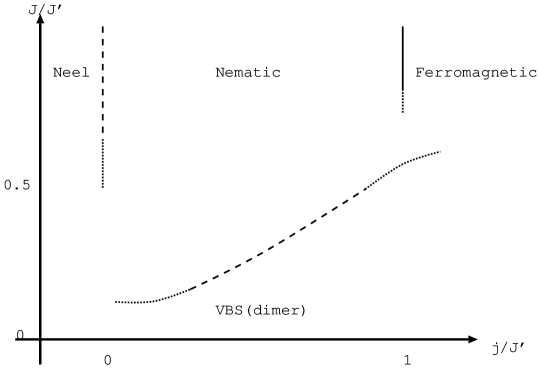
Figure 1: A schematic phase diagram for the $S=1$-spin model on the spatially anisotropic triangular lattice with the biquadratic interaction, Eq. (1), is presented. The limiting cases $J=0$ and $J\to\infty$ were studied in Refs. [20] and [21], respectively. The solid (dashed) lines stand for the phase boundaries of discontinuous (continuous) character. The dotted lines are ambiguous. We investigate the phase boundary separating the nematic and VBS phases.

Figure 2: (a) We consider a spatially anisotropic triangular lattice; the Hamiltonian is given by Eq. (1). The interaction $J$ interpolate the one- and two-dimensional lattice structures in the limiting cases of $J=0$ and $J\to\infty$, respectively. (b) In order to take into account such a geometrical character, we implement the screw-boundary condition. As shown in the drawing, a basic structure of the cluster is an alignment of spins $\{{\bf S}_{i}\}$ ($i\leq N$). Thereby, the dimensionality is lifted to $d=2$ by the bridges over the ($\sqrt{N}$)-th neighbor pairs through the $J$ bonds. Technical details are explained in Section 2.1.

Figure 3: The Binder parameter for the VBS-order parameter $U_{V}$ (8) is plotted for various $J$ and $N=$ ($+$) $10$, ($\times$) $12$, ($*$) $14$, ($\Box$) $16$, ($\blacksquare$) $18$, and ($\circ$) $20$. The parameter $j$ is set to $j=0.5$. ($J^{\prime}$ is the unit of energy.) The VBS order develops in the small-$J$ side.

Figure 4: The approximate critical point $J_{c}^{\alpha}(N_{1},N_{2})$ (10) is plotted for $[2/(N_{1}+N_{2})]^{2}$ ($10\leq N_{1}<N_{2}\leq 20$) with $\alpha=V$ (plusses) and $\alpha=Q$ (crosses). The parameters are the same as those of Fig. 3. The least-squares fit to these data yields $J_{c}^{V}=0.236(18)$ and $J_{c}^{Q}=0.151(11)$, respectively, in the thermodynamic limit.

Figure 5: The approximate critical exponent $\nu^{\alpha}(N_{1},N_{2})$ (11) is plotted for $[2/(N_{1}+N_{2})]^{2}$ ($10\leq N_{1}<N_{2}\leq 20$) with $\alpha=V$ (plusses) and $\alpha=Q$ (crosses). The parameters are the same as those of Fig. 3. The least-squares fit to these data yields $\nu^{V}=1.001(93)$ and $\nu^{Q}=0.902(45)$, respectively, in the thermodynamic limit.

Figure 6: The Binder parameter for the nematic- (quadrupolar-) order parameter $U_{Q}$ (12) is plotted for various $J$ and $N=$ ($+$) $10$, ($\times$) $12$, ($*$) $14$, ($\Box$) $16$, ($\blacksquare$) $18$, and ($\circ$) $20$. The parameters are the same as those of Fig. 3. The nematic order develops in the large-$J$ side.

Figure 7: The approximate critical exponent $\eta_{V}^{\alpha}(N_{1},N_{2})$ (14) is plotted for $[2/(N_{1}+N_{2})]^{2}$ ($10\leq N_{1}<N_{2}\leq 20$) with $\alpha=V$ (pluses) and $\alpha=Q$ (crosses). The parameters are the same as those of Fig. 3. The least-squares fit to these data yields $\eta_{V}^{V}=0.786(38)$ and $\eta^{Q}_{V}=-0.12(16)$, respectively, in the thermodynamic limit.

Figure 8: The approximate critical exponent $\eta_{Q}^{\alpha}(N_{1},N_{2})$ (15) is plotted for $[2/(N_{1}+N_{2})]^{2}$ ($10\leq N_{1}<N_{2}\leq 20$) with $\alpha=V$ (pluses) and $\alpha=Q$ (crosses). The parameters are the same as those of Fig. 3. The least-squares fit to these data yields $\eta^{V}_{Q}=-0.141(94)$ and $\eta_{Q}^{Q}=-0.089(18)$, respectively, in the thermodynamic limit.

References

• [1] T. Senthil, A. Vishwanath, L. Balents, S. Sachdev, and M. P. A. Fisher, Science 303 (2004) 1490.
• [2] T. Senthil, L. Balents, S. Sachdev, A. Vishwanath, and M. P. A. Fisher, Phys. Rev. B 70 (2004) 144407.
• [3] M. Levin and T. Senthil, Phys. Rev. B 70 (2004) 220403.
• [4] A. W. Sandvik, Phys. Rev. Lett. 98 (2007) 227202.
• [5] R. G. Melko and R. K. Kaul, Phys. Rev. Lett. 100 (2008) 017203.
• [6] V. N. Kotov, D.-X. Yao, A. H. Castro Neto, and D. K. Campbell, Phys. Rev. B 80 (2009) 174403.
• [7] L. Isaev, G. Ortiz, and J. Dukelsky. Phys. Rev. B 82 (2010) 136401.
• [8] V. N. Kotov, D.-X. Yao, A. H. Castro Neto, and D. K. Campbell, Phys. Rev. B 82 (2010) 136402.
• [9] L. Isaev, G. Ortiz, and J. Dukelsky, J. Phys.: Condens. Matter 22 (2010) 016006.
• [10] A. Kuklov, N. Prokof’ev, and B. Svistunov, Phys. Rev. Lett. 93 (2004) 230402.
• [11] A.B. Kuklov, M. Matsumoto, N.V. Prokof’ev, B.V. Svistunov, and M. Troyer, Phys. Rev. Lett. 101 (2008) 050405.
• [12] F.-J. Jiang, M. Nyfeler, S. Chandrasekharan, and U.-J. Wiese, J. Stat. Mech. (2008) P02009.
• [13] K. KrΓΌger and S. Scheidl, Europhys. Lett. 74 (2006) 896.
• [14] J. Sirker, Z. Weihong, O.P. Sushkov, and J. Oitmaa, Phys. Rev. B 73 (2006) 184420.
• [15] D. Poilblanc, A. LΓ€uchli, M. Mambrini, and F. Mila, Phys. Rev. B 73 (2006) 100403(R).
• [16] Y. Nishiyama, Phys. Rev. B 85 (2012) 014403.
• [17] K. Harada, N. Kawashima, and M. Troyer, J. Phys. Soc. Japan 76 (2007) 013703.
• [18] Y. Nishiyama, Phys. Rev. B 79 (2009) 054425.
• [19] Y. Nishiyama, Phys. Rev. B 83 (2011) 054417.
• [20] G. FΓ‘th and J. SΓ³lyom, Phys. Rev. B 51 (1995) 3620.
• [21] K. Harada and N. Kawashima, Phys. Rev. B 65 (2002) 052403.
• [22] M. A. Novotny, J. Appl. Phys. 67 (1992) 5448.
• [23] Y. Nishiyama, Phys. Rev. E 78 (2008) 021135.
• [24] N. Read and S. Sachdev, Phys. Rev. Lett. 62 (1989) 1694.
• [25] N. Kawashima and Y. Tanabe, Phys. Rev. Lett. 98 (2007) 057202.
• [26] J. Lou, A. W. Sandvik, and N. Kawashima, Phys. Rev. B 80 (2009) 180414(R).
• [27] R. K. Kaul, Phys. Rev. B 84 (2011) 054407.
• [28] K. S. D. Beach, F. Alet, M. Mambrini, and S. Capponi, Phys. Rev. B 80 (2009) 184401.
• [29] J. Lou and A. W. Sandvik, Phys. Rev. B 80 (2009) 212406.
• [30] T. Grover and T. Senthil, Phys. Rev. Lett. 107 (2011) 077203.
• [31] O. I. Motrunich and A. Vishwanath, Phys. Rev. B 70 (2004) 075104.
• [32] M. Campostrini, M. Hasenbusch, A. Pelissetto, P. Rossi, and E. Vicari, Phys. Rev. B 65 (2002) 144520.
• [33] E. Manousakis, Rev. Mod. Phys. 63 (1991) 1.
• [34] A. Banerjee, K. Damle, and F. Alet, Phys. Rev. B 82 (2010) 155139.