Background X-ray Radiation Fields Produced by
Young Embedded Star Clusters

Abstract

Most star formation in our galaxy occurs within embedded clusters, and these background environments can affect the star and planet formation processes occurring within them. In turn, young stellar members can shape the background environment and thereby provide a feedback mechanism. This work explores one aspect of stellar feedback by quantifying the background X-ray radiation fields produced by young stellar objects. Specifically, the distributions of X-ray luminosities and X-ray fluxes produced by cluster environments are constructed as a function of cluster membership size $N$. Composite flux distributions, for given distributions of cluster sizes $N$, are also constructed. The resulting distributions are wide and the X-ray radiation fields are moderately intense, with the expected flux levels exceeding the cosmic and galactic X-ray backgrounds by factors of $\sim 10-1000$ (for energies 0.2 – 15 keV). For circumstellar disks that are geometrically thin and optically thick, the X-ray flux from the background cluster dominates that provided by a typical central star in the outer disk where $r\gtrsim 9-14$ AU. In addition, the expectation value of the ionization rate provided by the cluster X-ray background is $\zeta_{X}\sim 8\times 10^{-17}$ s^-1, about 4 – 8 times larger than the canonical value of the ionization rate from cosmic rays. These elevated flux levels in clusters indicate that X-rays can affect ionization, chemistry, and heating in circumstellar disks and in the material between young stellar objects.

1 Introduction

Most star formation in our galaxy occurs within embedded clusters, which are themselves located inside giant molecular clouds. The radiation fields produced by these stellar nurseries can influence the formation of additional cluster members, and especially their accompanying planetary systems (Adams 2010). More specifically, the processes of star and planet formation can be affected via [1] heating of starless cores, leading to evaporation and the loss of star forming potential (e.g., Gorti & Hollenbach 2002), [2] ionization within starless cores, leading to greater coupling between the magnetic fields and gas (e.g., Shu 1992), thereby acting to suppress continued star formation, [3] evaporation of circumstellar disks, leading to loss of planet forming potential (e.g., Shu et al. 1993, Hollenbach et al. 1994, Störzer & Hollenbach 1999, Adams et al. 2004), and [4] ionization of circumstellar disks, which helps maintain the magneto-rotational instability (MRI), which in turn helps drive disk accretion (e.g., Balbus & Hawley 1991). With regard to circumstellar disks, we note that the background radiation from the cluster environment often dominates that produced by the central star, especially at ultraviolet (UV) wavelengths (e.g., Hollenbach et al. 2000; Armitage 2000; Adams & Myers 2001, Fatuzzo & Adams 2008); nonetheless, the photoevaporation of disks is often driven by stellar radiation (e.g., Shu et al. 1993; Alexander et al. 2004, 2005, 2006).

Multi-wavelength observations of embedded clusters over the past two decades have provided a wealth of information on these environments (Lada & Lada 2003; Porras et al. 2003; Allen et al. 2007), making it possible to assess what impact a given physical process can have on star and planet formation. Indeed, a comprehensive analysis of the effects of FUV and EUV background fields on cluster environments has already been performed (Armitage 2000; Adams et al. 2006; Fatuzzo & Adams 2008; Hollenbach & Gorti 2009; Holden et al. 2010). The main goal of this paper is to perform a similar analysis for the X-ray band.

This paper is organized as follows. In Section 2, we discuss the cluster environment, present our characterization of the stellar IMF, and outline the basic approach for assigning X-ray luminosities to stars in our cluster models. We discuss the statistical aspects of our cluster model in Section 3 and present distributions of the X-ray luminosities for clusters with varying stellar membership size $N$. In Section 4, we construct the corresponding distributions of X-ray fluxes, both for varying $N$ and for different forms for the stellar density profiles. The implications of these findings are discussed in Section 5; the paper concludes in Section 6 with a summary of results and a discussion of potential applications.

2 The Cluster Environment

Studies of clusters out to 2 kpc (Lada & Lada 2003) and out to 1 kpc (Porras et al. 2003) indicate that in the solar neighborhood, the number of stars born in clusters with $N$ members is (almost) evenly distributed logarithmically over the range $N\approx$ 30 to 3000, with half of all stars belonging to clusters with $N\lesssim 300$. These stars are contained within a cluster radius $R_{c}$ ranging between $0.1-2$ pc, with the radial sizes of observed clusters following an empirically determined law of the form

$${R_{\rm c}}(N)=1\,{\rm pc}\,\left({N\over 300}\right)^{\gamma}\,,$$ (1)

with $\gamma=1/2$ (see Figure 2 of Adams et al. 2006, which uses the data from Carpenter 2000 and Lada & Lada 2003). For simplicity, we adopt this relation to specify the cluster radius throughout most of this paper, although we use $\gamma=1/3$ when considering a population of clusters that extend up to $N=10^{5}$ in order to be consistent with the radial sizes observed for larger clusters (for further discussion and supporting data, see Chandar et al. 1999; Pfalzner 2009; Proszkow & Adams 2009). The gas within the cluster environment not used to build stars accounts for roughly 70 – 90% of the total (gas and stellar) mass of the cluster, and extends well beyond $R_{c}$ until it eventually merges smoothly into the background of the molecular cloud.

We assume that the stars within a cluster are drawn from a parent population that is described by the universal initial mass function (IMF) observed in our Galaxy. The resulting probability distribution is therefore independent of membership size $N$. We adopt the broken power-law form of the IMF presented in Kroupa (2001; not corrected for binaries), expressed in terms of dimensionless mass $m=M/M_{\odot}$ and truncated at $m=100$, so that

$${dN_{\star}\over dm}=C_{i}\,m^{-\alpha_{i}}\,,$$ (2)

where

$$\alpha_{0}=0.3 \qquad 0.01\leq m\leq 0.08\,,$$

$$\alpha_{1}=1.3 \qquad 0.08\leq m\leq 0.5\,,$$ (3)

$$\alpha_{2}=2.3 \qquad 0.5\leq m\leq 100\,.$$

The constants $C_{i}$ are easily determined through the continuity of the IMF and the normalization of equation (2) to the number of stars within a cluster. For completeness, we note that the expectation value of the stellar mass for the adopted IMF is given by

$$\langle m\rangle\equiv{1\over N_{\star}}\int_{0.01}^{100}m\,\left({dN_{\star}\over dm}\right)\,dm=0.38\,,$$ (4)

where $N_{\star}$ = $\int(dN_{\star}/dm)dm$.

We now consider the X-ray luminosity of the stars within an embedded cluster. X-rays from low-mass stars ($m\lesssim 2$) are produced from flaring events in stellar coronae, whereas X-ray emission from high-mass stars ($m\gtrsim 18$) is driven by stellar winds (intermediate mass stars most likely do not produce X-rays, with detections from such stars then attributed to low-mass companions). It is not surprising, therefore, that observations of X-ray luminosities of cluster members show a large variance in X-ray values (e.g, Feigelson et al. 1993, Feigelson et al. 2002, Preibisch et al. 2005); the variance also tends to decrease with the cluster age (see Alexander & Preibisch 2012). Nonetheless, these observations indicate that the X-ray luminosity depends on stellar mass. Modeling the exact nature of this dependence is hampered by the large variance in the data and by the fact that the derived correlation between $L_{X}$ and $m$ is model dependent (Preibisch 2005). In our work, we adopt a purely empirical approach and use a monotonic relation between stellar mass and X-ray luminosity. Specifically, we use the results obtained by Preibish et al. (2005), and focus primarily on the PS model for which a linear regression fit yields the relation

$$\log\left(L_{X}[\rm{erg\,s}^{-1}]\right)=30.34+1.13\,\log m\;,$$ (5)

and a standard deviation of $\Delta(\log L_{X})=0.64$. As shown in Figure 1, this best fit line (solid line) and the corresponding $\pm\Delta(\log L_{X})$ deviations (dotted lines) are in reasonable agreement with the low-mass data (squares) obtained from Chamaeleon I (Feigelson et al. 1993) and the low-mass data (gray area) and intermediated/high-mass data (circles) obtained from the Orion Nebula (Feigelson et al. 2002). For completeness, we also calculate cluster luminosity distributions using results from the SDF models, for which a linear regression fit yields the relation

$$\log\left(L_{X}[\rm{erg\,s}^{-1}]\right)=30.37+1.44\,\log m\;,$$ (6)

and a standard deviation of $\Delta(\log L_{X})=0.65$.

As elaborated on in Section 3, we obtain X-ray luminosity distributions for clusters with $N$ members by randomly sampling the IMF for each stellar member, and then assigning a luminosity to each star based on its mass. For a fixed stellar mass, we include a distribution of X-ray luminosities; guided by the aforementioned observations, this latter step is performed by randomly selecting a value of $\log\left[L_{X}(m)\right]$ from a normal distribution with the mean given by equation (5) or equation (6) and with a standard deviation $w$ $\equiv\Delta(\log L_{X})$. We note that for the PS model, the mean luminosity of the resulting distribution for stars of mass $m$ is

$$\bar{L}_{X}(m)\,[{\rm erg\,s}^{-1}]=\int_{-\infty}^{\infty}P[x;30.34+1.13\log m,0.64]10^{x}dx=6.4\times 10^{30}\,m^{1.13}\;,$$ (7)

where $P[x;\mu,w]$ is the probability density function of mean $\mu$ and standard deviation $w$. This value is denoted by the dashed line in Figure 1. Since the values of $\log\left[L_{X}(m)\right]$ are selected from a normal distribution, the corresponding distribution of $L_{X}$ values are not normal, but rather, are positively skewed. As a result, $\log\bar{L}_{X}(m)>30.34+1.13\log m$ (as seen in Figure 1). The expectation value of the X-ray luminosity — per star — over the full distribution of stellar masses is then given by

$${\langle L_{X}\rangle_{\ast}}\equiv{1\over N}\int_{0.01}^{100}\bar{L}_{X}(m)\,{dN_{\star}\over dm}\,dm=2.6\times 10^{30}\;{\rm erg\,s}^{-1}.$$ (8)

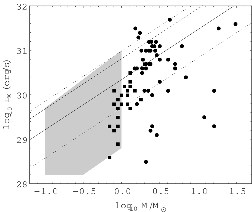
Figure 1: Summary of observational data for the mass vs X-ray luminosity relation for stars in young cluster environments. Squares – low mass Chamaeleon I stars presented in Table 6 of Feigelson et al. (1993); circles – intermediate/high mass ONC stars presented in Table 5 of Feigelson et al. (2002); grey region – region of parameter space spanned by soft X-ray emission of low mass ONC stars, as presented in Figure 14 of Feigelson et al. (2002). The solid line shows the results of the linear regression fit obtained by Preibish et al. (2005) using the PS model, and the dotted lines mark the corresponding $\pm w$ deviations, where $w=\Delta(\log L_{X})$ is the residual standard deviation. The dashed line represents the mean value $\bar{L}_{X}(m)$ as given by equation (7) in the text.

We next consider the contribution to the total X-ray luminosity that comes from stars with mass $m$ for a parent population drawn from our adopted IMF. We start by noting that the function

$$\psi_{X}(m)\equiv\bar{L}_{X}(m)\,{dN_{\star}\over dm}\,,$$ (9)

which characterizes the X-ray luminosity produced by the stellar population (as a function of mass), peaks at $m=0.08$ and drops off as a power-law $\psi_{X}\propto m^{-1.17}$ for masses $m>0.5$. As a result, most of the luminosity of a cluster per mass decade, which scales as $m\psi_{X}$, is expected to come from stars with mass $m\gtrsim 0.5$. To illustrate this point, we randomly select $10^{7}$ stars from our IMF and then select the corresponding luminosity from equation (5), including the variance about this mean relationship as prescribed above. The resulting X-ray luminosity distribution is shown in Figure 2. The distribution displays a broad peak near $L_{X}\sim 10^{29}$ erg s^-1 $\approx\bar{L}_{X}(0.08)$, and approaches a slope of $-1$ (as indicated by the dotted line) as $L_{X}\rightarrow 10^{31}$ erg s^-1 $\sim\bar{L}_{X}(0.5)$. The distribution of X-ray luminosity per mass decade at higher values is therefore nearly flat, indicating that above $m\approx 0.5$, stars ranging in mass between $m=10\rightarrow 100$, although fewer in number, can contribute nearly the same to the total cluster X-ray luminosity as stars ranging in mass between $m=1\rightarrow 10$. This result is consistent with the weak dependence of the function $m\psi_{X}\propto m^{-0.17}$ on mass above $m=0.5$. It is worth noting that our calculated distribution, as shown in Figure 2, is in good agreement with the observed distribution of X-ray luminosities of the Orion Nebula population (see Figure 3a in Feigelson et al. 2005).

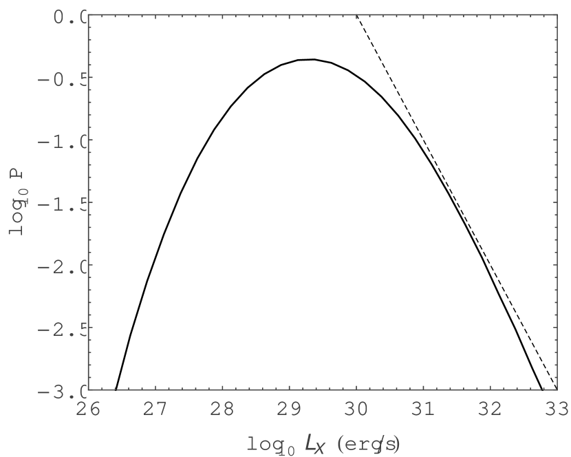
Figure 2: Probability distribution of the X-ray luminosities. This distribution was obtained by first randomly selecting a stellar mass from the IMF defined by equations (2) and (2), and then obtaining the corresponding luminosity by randomly selecting $L_{X}$ from a normal distribution of $\log L_{X}$ with mean given by equation (5) and standard deviation $w=\Delta(\log L_{X})=0.64$ as discussed in the text. The dotted line has slope –1 and is included for illustrative purpose.

3 X-Ray Luminosity Distributions

With the IMF and the prescription for obtaining the luminosity of the sources specified, we now determine the characteristics of the X-ray luminosity distribution for a given cluster of size $N$, including both the expectation value and the variance. The X-ray luminosity for a single cluster, denoted as $L_{X}(N)$, is given by the sum

$$L_{X}(N)=\sum_{j=1}^{N}L_{Xj}\,,$$ (10)

where $L_{Xj}$ is the X-ray luminosity from the $jth$ member, and $N$ is the membership size of the cluster. In this formulation, we assume that the X-ray luminosity for a given star is determined by a distribution whose properties depend only on the stellar mass, and that the stellar mass is drawn independently from the specified stellar IMF. The sum in equation (10) is thus the sum of random variables, where the variables are drawn from known and independent distributions (which are determined by the IMF and the $L_{X}-m$ relation). In the limit of large $N$, the expectation value ${\langle L_{X}\rangle_{C}}$ of the X-ray power for the cluster (which is a function of $N$) is given by the expression

$${\langle L_{X}\rangle_{C}}=N{\langle L_{X}\rangle_{\ast}}\,,$$ (11)

where ${\langle L_{X}\rangle_{\ast}}$ is the expectation value of the X-ray power per star, as given by equation (8). As usual, the central limit theorem implies that the distribution of values $L_{X}(N)$ obtained by sampling over many clusters must approach a Gaussian form in the limit $N\to\infty$ (e.g., Richtmyer 1978), although convergence is often slow. One of the issues of interest here is the value of stellar membership $N$ required for these statistical considerations to be valid; similarly, we would like to know the fraction of the cluster population that has such sufficiently large $N$. In its limit of applicability, this Gaussian form for the composite distribution is independent of the form of the initial distributions, i.e., the shape of the distribution is independent of the stellar IMF and the mass-luminosity relation. The width of the distribution also converges to a known value given by the expression

$$\langle w\rangle_{X}^{2}={1\over N}\sum_{j=1}^{N}w_{j}^{2}\quad\Rightarrow\quad\langle w\rangle_{X}=\sqrt{N}w_{0}\,,$$ (12)

where $w_{0}$ is the width of the individual distribution, i.e.,

$$w_{0}^{2}\equiv\langle L_{X}^{2}\rangle_{\ast}-{\langle L_{X}\rangle_{\ast}}^{2}\,.$$ (13)

We can write $w_{0}=Q{\langle L_{X}\rangle_{\ast}}$, where $Q$ is the dimensionless width of the X-ray luminosity distribution. Using the specifications given above, we find $Q\approx 17$. For a given membership size $N$, the mean value of the distribution of cluster luminosities converges to the value $N\langle{L_{X}}\rangle_{\ast}$, whereas the width of the distribution converges to $\sqrt{N}Q\langle{L_{X}}\rangle_{\ast}$. As a result, the mean value will be larger than the width of the distribution only if the number of stellar members exceeds $N_{Q}=Q^{2}\approx 300$. Small clusters (with $N<N_{Q}\approx 300$) thus have such wide distributions of X-ray luminosity that the mean value does not provide a good estimate. For larger clusters (with $N>N_{Q}$), the X-ray luminosity is adequately characterized by the expectation value, but the distributions retain significant (relative) widths. These trends are illustrated in the figures that follow below.

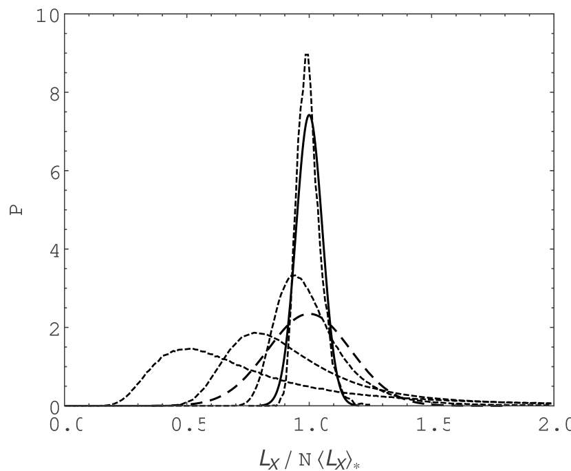
Figure 3: Distribution of X-ray luminosities. The short-dashed curves show the probability distributions for clusters with (from left to right) $N=10^{2}$ stars, $N$ = $10^{3}$ stars, $N=10^{4}$ stars, and $N=10^{5}$ stars. Note that the luminosities (along the horizontal axis) are normalized by the average value one would obtain with complete sampling of the stellar IMF. For comparison, the long-dashed curve shows a Gaussian distribution with mean $\mu=1$ and standard deviation $w=Q/\sqrt{10^{4}}$, and the solid curve shows a Gaussian distribution with mean $\mu=1$ and standard deviation $w=Q/\sqrt{10^{5}}$.

Figure 3 illustrates the X-ray luminosity distributions obtained from our cluster model, scaled by the cluster expectation value $N{\langle L_{X}\rangle_{\ast}}$ from equation (11), for clusters with membership size $N=10^{2}$, $10^{3}$, $10^{4}$, and $10^{5}$ (short-dashed curves, from left to right). The long-dashed curve represents a Gaussian profile with mean $\mu=1$ and standard deviation $w=Q/\sqrt{10^{4}}$, whereas the solid curve represents a Gaussian profile with mean $\mu=1$ and standard deviation $w=Q/\sqrt{10^{5}}$. It is clear from this result that as $N$ increases, the sampling becomes more complete, and the distributions approach a Gaussian form. However, in practice, even with large values of cluster membership size $N$, the asymptotic form is not reached. We note that the clusters in our solar neighborhood, as observed by Lada & Lada (2003) and Porras et al. (2003), are in the regime of incomplete sampling, and the distributions of their X-ray luminosities are expected to have median values that are smaller than $N{\langle L_{X}\rangle_{\ast}}$ while retaining significant tails.

Figure 4 shows the X-ray luminosity distributions (with physical units) for clusters with stellar membership size $N$ = 100, 300, 1000, 3000 and 10000, constructed using both the PS model (solid curves) and the SDF model (dashed curves) for the X-ray luminosity vs mass relation. As expected, the mean/median values of the distributions increase with increasing $N$; in addition, the width of the distribution decreases with increasing $N$. The SDF models produce distributions with larger means and standard deviations (by about a factor of 2 for larger clusters) than their PS model counterparts. These characteristics result from the stronger mass dependence for the luminosity in the SDF models, resulting in a broader range of luminosity values sampled in that case.

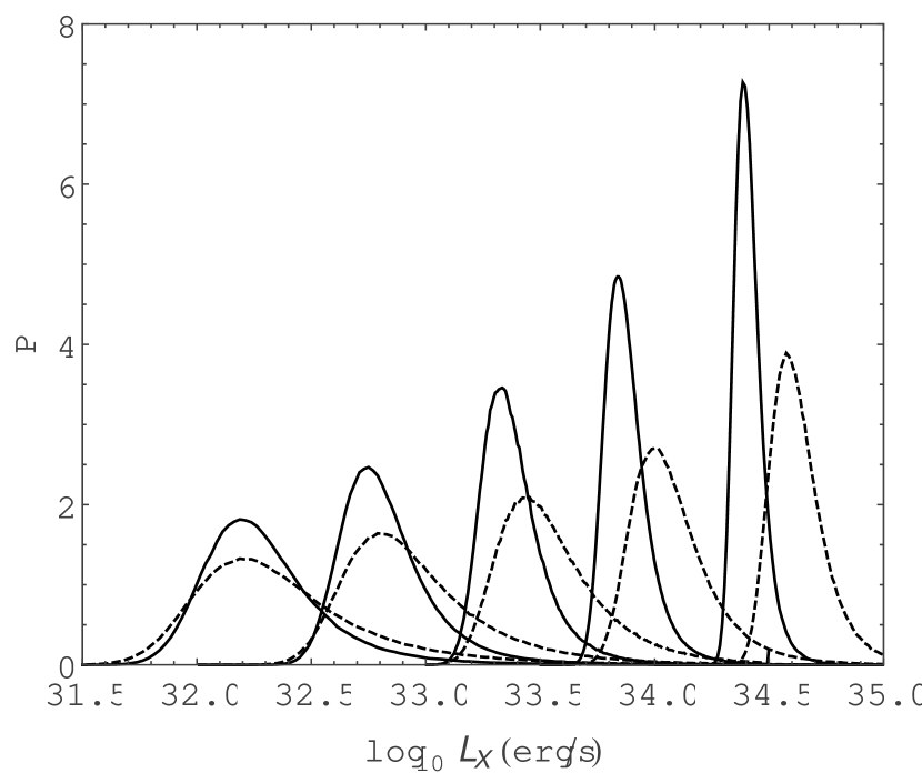
Figure 4: Probability distribution for X-ray luminosities. The five pairs of curves show the probability distributions for clusters of size (from left to right) $N$ = 100, 300, 1000, 3000 and 10000. Solid curves were obtained using the PS model; dashed curves were obtained using the SDF model.

4 X-Ray Flux Distributions

In this section we construct distributions of the X-ray flux impinging upon the cluster members. Unlike the FUV and EUV bands, for which a significant fraction of the luminosity is produced by the most massive member of the cluster (e.g., Fatuzzo & Adams 2008), the total X-ray luminosity can arise from comparable contributions of numerous stars. As a result, the overall X-ray emission can be spread out over the entire cluster region, although this assumption is not universally true. For example, about 50% of the total X-ray luminosity from all ($N\gtrsim 1500$) of the X-ray emitting stars in the Orion Nebula Cluster comes from the most massive star. Nevertheless, we can obtain a benchmark estimate for the X-ray flux within the cluster environment by dividing the expectation value of the luminosity $N{\langle L_{X}\rangle_{\ast}}$ by the fiducial surface area $A$ = $\pi R_{c}(N)^{2}$, where $R_{c}(N)$ is given by equation (1), which yields a value of

$$F_{X0}={N{\langle L_{X}\rangle_{\ast}}\over\pi R_{c}(N)^{2}}=2.6\times 10^{-5}\,{\rm erg}\,{\rm cm}^{-2}\,{\rm s}^{-1}\;.$$ (14)

Of course, the X-ray fluxes within a cluster, and within a collection of clusters, will take on a distribution of values, where $F_{X0}$ represents an order-of-magnitude estimate for the mean. In order to construct these distributions of the X-ray flux, we first randomly select the position of a test star within a radius $R_{c}(N)$ (assuming a spherical distribution), weighted by a chosen density profile. For this study, we consider density profiles with the simple forms $\rho\propto 1/r$ and $\rho\propto 1/r^{2}$; these profiles roughly bracket the possible profiles expected from observations. The probability that the test star is located a distance between $r$ and $r+dr$ from the cluster center is then given by

$$P(r)\,dr={\rho\,r^{2}dr\over\int_{0}^{R_{c}}\rho\,r^{2}dr}\;.$$ (15)

We then randomly selected the positions of the remaining $N-1$ stars within the cluster, following the same prescription used to set the location of the test star. For each of these field stars, a luminosity is obtained as detailed in Section 2. The flux impinging on the test star is calculated, and the entire process is then repeated $10^{7}$ times in order to build up flux distributions. Note that this procedure builds a slightly different distribution than the one that describes the flux values found within the cluster environment, for which case the location of the test star (which was weighted in accordance to the specified density profile) would have been replaced by a randomly selected location within the cluster that was not weighted by the density profile.

The results are shown in Figure 5 (for $\rho\sim 1/r$) and in Figure 6 (for $\rho\sim 1/r^{2}$). The range of fluxes realized within the clusters is comparable to (but generally less than) the benchmark estimate of equation (14). Note that the flux distributions peak at nearly the same locations for both density profiles (we use the same expression to set the cluster radius for both cases, so that the mean stellar density for a given cluster size $N$ is the same for both density profiles). However, stars with a $\rho\propto 1/r^{2}$ profile are more centrally localized, leading to a distribution that extends out to higher values of flux. As the stellar membership size $N$ increases, sampling of the stellar IMF becomes more complete, and the flux distributions shift to higher values (they move to the right in the figures) and become somewhat narrower. In rough terms, however, the expected X-ray flux levels are given by $F_{X}\sim 10^{-5}$ erg cm^-2 s^-1, with a factor of $\sim 3-4$ variation for $\rho\propto 1/r$ profiles and $\sim 5-10$ variations (above the peak) for $\rho\propto 1/r^{2}$ profiles.

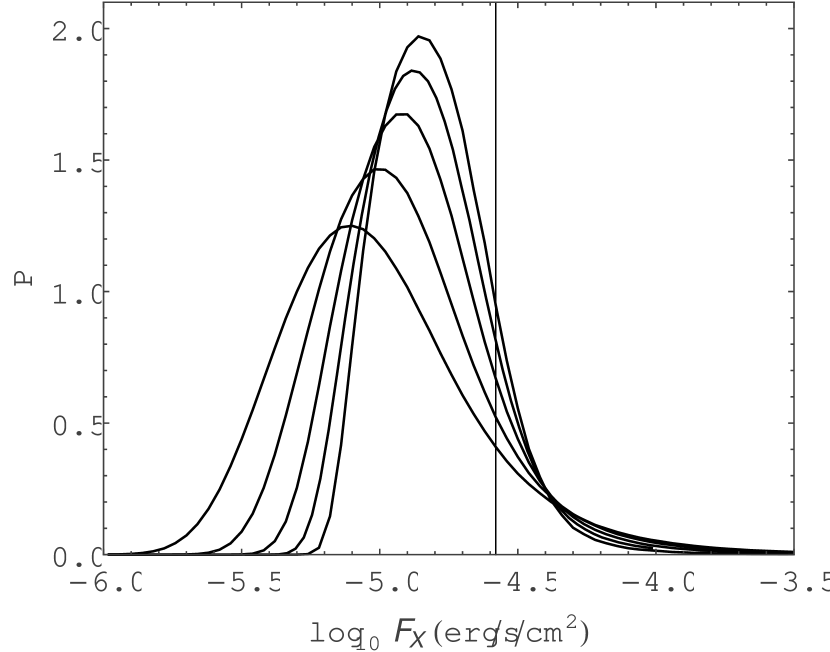
Figure 5: Probability distribution for the X-ray flux impinging upon stellar members for clusters where the stars follow a radial density distribution $\rho\propto 1/r$. The five curves show the probability distributions (left to right) for clusters with varying membership sizes $N$ = 100, 300, 1000, 3000 and 10000. The vertical line denotes our benchmark value of X-ray flux defined by equation (14).

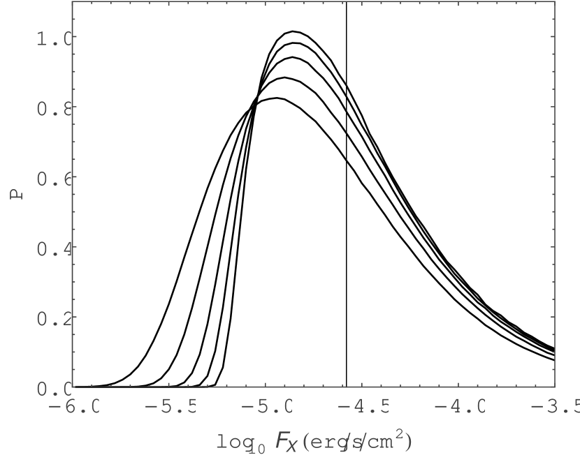
Figure 6: Same as Figure 5, but for stars following a radial density distribution with $\rho\propto 1/r^{2}$.

We complete our analysis by constructing composite flux distributions for all stars within: i) a cluster population similar to that observed in our solar neighborhood, for which the largest cluster has $N_{max}$ = 3000 stars; and ii) a cluster population with cluster membership size extending up to $N_{max}=10^{5}$. For case (i) we assume a cluster radius as specified by equation (1) with $\gamma$ = 1/2, whereas for case (ii) we assume $\gamma$ = 1/3. Following the observational result that clusters in the solar neighborhood have sizes $N$ that are (almost) evenly distributed logarithmically, we assume that both populations are described by the cumulative distribution

$$f(N)={\log(N)-\log(30)\over\log(N_{max})-\log(30)}\,,$$ (16)

where $f(N)$ denotes the fraction of stars born in clusters of stellar membership less than or equal to $N$ (see, e.g., Figure 1 from Fatuzzo & Adams 2008). Note that for $N_{max}=3000$, $f(300)=0.5$, so that half of the stars in the entire cluster population belong to clusters with $N\leq 300$; for comparison, this “median point” is much larger for the sample with $N_{max}=10^{5}$, where $f(1732)$ = 0.5. Composite distributions are then obtained by first sampling over the assumed cluster population to set the size of the cluster that our test star belongs to, and then performing the process outlined above to calculate the flux impinging on that star as a result of the other stellar members. This process is then repeated $10^{7}$ times in order to build up a statistically valid distribution. The results are presented in Figures 7 and 8.

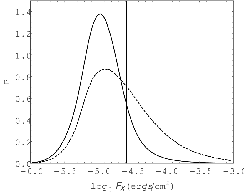
Figure 7: Composite distribution for the X-ray flux impinging upon stellar members in a population of clusters similar to that observed in the solar neighborhood with $N_{max}=3000$. The solid curve was obtained by assuming a density profile of the form $\rho\propto 1/r$. The dashed curve was obtained by assuming a density profile of the form $\rho\propto 1/r^{2}$. The vertical line denotes our benchmark value of flux as defined by equation (14).

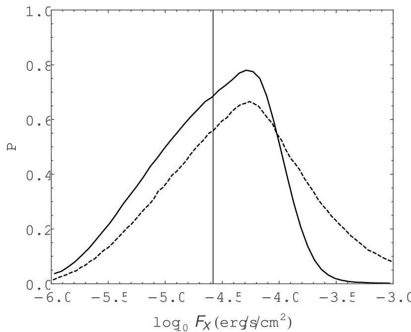
Figure 8: Same as Figure 7, but for a population of clusters with membership size extending up to $N_{max}=10^{5}$, and with radii given by equation (1) where $\gamma=1/3$.

5 Implications and Discussion

With the X-ray flux distributions specified, we can now assess some of the corresponding effects on the cluster and on forming stars (and planetary systems). We first compare the X-ray flux received by circumstellar disks from the background cluster with that received from their central stars. If we ignore geometry, the sphere of influence of the central star (in X-rays) is defined by the radius where the X-ray flux provided by the background environment $F_{XC}$ of the cluster is equal to that provided by the star $F_{X\star}$, i.e.,

$$F_{X\star}={L_{X}\over 4\pi r^{2}}=0.039\,\,{\rm erg}\,\,{\rm cm}^{-2}\,\,{\rm s}^{-1}\left({L_{X}\over 10^{29}\,\,{\rm erg}\,\,{\rm s}^{-1}}\right)\left({r\over 30\,\,{\rm AU}}\right)^{-2}=F_{XC}\,,$$ (17)

where we have scaled the X-ray luminosity to a typical value. For moderate-sized clusters with $N\leq N_{max}=3000$ such as those found in the solar neighborhood, and for $\rho\propto 1/r$ density profiles, the X-ray flux provided by the background cluster has a characteristic value $F_{XC}\approx 2\times 10^{-5}$ erg cm^-2 s^-1, but varies by factors of $3-4$ on either side of this benchmark (see Figures 5 and 7). For clusters with $\rho\propto 1/r^{2}$ density profiles, the X-ray flux has nearly the same peak value, but varies by factors of $5-10$ (see Figure 6). As a result, the sphere of influence of the star (in X-rays) extends out to about $r\approx 1300$ AU, much larger than the typical disk size. If we extend the cluster sample to larger membership sizes with $N_{max}=10^{5}$, the characteristic value of the X-ray flux increases to $F_{XC}\approx 6\times 10^{-5}$ erg cm^-2 s^-1 (see Figure 8) and the sphere of influence of the star has radius $r\approx 760$ AU, still somewhat larger than most circumstellar disks.

Taken at face value, this finding would indicate that the X-ray flux for the planet-forming region of the disk is (usually) dominated by the central star rather than the background environment of the cluster. However, this comparison ignores geometrical factors arising because the disk is not perpendicular to the outgoing stellar radiation. The expected vertical extent $\Delta z$ of the disk, in the context of X-ray absorption, is estimated to be $(\Delta z)/r\approx 0.3-0.4$ (see Figure 1 of Gorti & Hollenbach 2009). As a result, the disks are relatively thin geometrically, and the intercepted X-ray flux will be significantly smaller than the value presented in equation (17). For the limiting case of a geometrically flat disk, the flux intercepted by the disk has the following radial dependence

$$F_{X}(r)={L_{X}\over 4\pi R_{\ast}^{2}}{1\over\pi}\left[\arcsin u-u\left(1-u^{2}\right)^{1/2}\right]\to{L_{X}\over 4\pi R_{\ast}^{2}}{2\over 3\pi}\left({R_{\ast}\over r}\right)^{3}\,,$$ (18)

where $u\equiv R_{\ast}/r$ and where we have taken the large radius limit to obtain the final expression (Adams & Shu 1986). Using this expression, we find that the central star dominates the X-ray flux only out to $r\approx 14$ AU (9 AU) for clusters distributions with $N_{max}$ = 3000 ($10^{5}$). For these systems, the outer disk thus receives more X-ray flux from the cluster than from the central star. As an example, consider radial position $r=30$ AU and the extended cluster distribution with $N_{max}=10^{5}$; the X-ray flux from the star (from equation [18]) is estimated as $F_{X}\approx$ $2\times 10^{-6}$ erg cm^-2 s^-1, 30 times smaller than the background radiation flux.

Although the background cluster can provide more X-ray flux to circumstellar disks than their central stars, the X-ray irradiation of the inner portions of the disks by coronal emission from young stars remains important. Several studies, complementary to the analysis of this paper, have addressed the process of photoevaporation driven by X-rays from the central star (e.g., Ercolano et al. 2008, 2009). The predicted mass loss rates can be substantial (typically of order $10^{-8}$ $M_{\odot}$ yr^-1) and most of the mass loss takes place at disk radii in the range 10 – 20 AU, near the transition where X-ray flux is dominated by the star (inside this radius) and the background cluster (outside).

On the scale of the cluster itself, ionization of the cluster gas is an important consideration. The main contribution to ionization in star forming regions is often taken to be cosmic rays, which have a fiducial ionization rate $\zeta_{CR}\approx 10^{-17}$ s^-1 (Shu 1992); more recent studies suggest a slightly higher value $\zeta_{CR}\approx 2.6\times 10^{-17}$ s^-1 (van der Tak & van Dishoeck 2000). For comparison, the ionization rate due to the X-ray background radiation is given by

$$\zeta_{X}={F_{X}\over E_{X}}\sigma(E_{X}){E_{X}\over\Delta\epsilon}J(\tau,x_{0})\,,$$ (19)

where $E_{X}\sim 1$ keV is the characteristic energy of the X-rays, $\sigma(E_{X})$ is the total photoelectic cross section (see the discussion of Glassgold et al. 2000), the function $J$ is an attenuation factor, which is, in turn, a function of the optical depth $\tau$ in X-rays, and the threshold value $x_{0}$ = $E_{0}/kT_{X}$ (given by the lowest energy $E_{0}$ of the X-rays under consideration and by the temperature $T_{X}$ of the emission region). The function $J$ is expected to be of order unity (Krolik & Kallman 1983) and we will take $J=1$ for simplicity. The remaining factor in equation (19) is the factor $E_{X}/(\Delta\epsilon)$, where $\Delta\epsilon\approx$ 35 eV is the energy required to make an ion pair. This ratio thus represents the enhancement factor resulting from individual X-rays making multiple ionizations (note that $E_{X}/(\Delta\epsilon)\sim 30$). A power-law fit to the cross section results in the form

$$\sigma(E_{X})=\sigma_{0}(E_{X}/1\,\,{\rm keV})^{-n}\,,$$ (20)

where the index $n$ = 2.485 and the fiducial value of the cross section $\sigma_{0}$ = $2.27\times 10^{-22}$ cm² (Glassgold et al. 1997). Putting all of the above results together, we find that to leading order the X-ray ionization rate becomes

$$\zeta_{X}\approx 8\times 10^{-17}\,\,{\rm s}^{-1}\,\,\left({F_{XC}\over 2\times 10^{-5}\,\,{\rm erg}\,\,{\rm cm}^{-2}\,\,{\rm s}^{-1}}\right)\,.$$ (21)

For the given background X-ray flux value, the X-ray ionization rate is larger than the cosmic ray ionization rate by a factor of $\sim 4-8$ (see also Lorenzani & Palla 2001). Keep in mind, however, that the cosmic ray ionization rate varies with galactocentric radius and with column density of the region (van der Tak & van Dishoeck 2000). Likewise, the X-ray fluxes have a broad distribution of values (as shown in Figures 5 – 8), so that the X-ray ionization rate can be much larger, or smaller, than the benchmark value given in equation (21). The relative importance of cosmic ray and X-rays for ionization is thus expected to vary significantly from cluster to cluster.

The cluster is essentially optically thin to X-rays, so that young stellar objects within the cluster receive the unattenuated flux. We can estimate the optical depth as follows: The cross section of equation (20) can be integrated over the energy range of the observational surveys (the energy range used to construct the flux distributions) to find an average value $\langle\sigma\rangle$ $\approx$ $\sigma_{0}/10\approx 2\times 10^{-23}$ cm². The number density $n$ of a cluster with $N$ = 100 – 1000 and radius $R_{c}\sim 1$ pc is about $n$ = 3000 cm^-3. The mean free path of an X-ray is thus $\ell=1/n\langle\sigma\rangle\approx 5{\rm pc}>R_{c}$.

Another way to gauge the importance of the X-ray radiation fields is to compare the flux levels to those of the background galaxy and the background universe. Here we are interested in X-rays in the range 0.2 – 15 keV, corresponding to the range in the observational surveys used to construct the X-ray luminosity vs mass relations used in this paper. The total flux in soft X-rays (in the range 0.28 – 1 keV) is estimated to lie in the range $f_{X}\approx 5-10\times 10^{-8}$ erg cm^-2 s^-1 (Fried et al. 1980), where we have assumed an isotropic radiation field to convert (energy-integrated) specific intensity to flux. This value has considerable uncertainty. In addition, comparable fluxes are present in harder X-rays, e.g., the range 1 – 15 keV that provides the other half of the range under consideration. These harder X-rays are thought to come from extragalactic sources (and are observed to be nearly isotropic), whereas the softer X-rays have a significant Galactic contribution (e.g., Boldt 1987). In any case, the total X-ray background flux is about $f_{X}\approx 1-2\times 10^{-7}$ erg cm^-2 s^-1. Given the distributions of cluster properties considered here, and the distributions of fluxes for a given type of cluster, the X-ray flux provided by clusters $F_{XC}$ is larger than the background $f_{X}$ by factors in the range 10 – 1000.

6 Conclusion

This paper constructs the expected X-ray radiation fields provided by young embedded clusters. Specifically, we calculate the distributions of X-ray luminosity for clusters of a given membership size $N$ and the corresponding distributions of X-ray flux. We also determine the distributions of X-ray flux for two cluster ensembles (for the cluster distribution found in the solar neighborhood and for an extended distribution with maximum membership size $N_{max}=10^{5}$). The flux distributions depend on the density profile of the stellar objects (the individual X-ray sources) within the cluster and we consider models that span the expected range of possibilities. The main results can be summarized as follows:

The expected flux levels for X-rays are modest, with a characteristic value of order $F_{X}\sim 1-6\times 10^{-5}$ erg cm^-2 s^-1; the range corresponds to the types of clusters under consideration, where the X-ray flux increases with cluster membership size $N$ and with the central concentration of the density profile (Figures 5 – 8). The distributions of X-ray flux are relatively wide, however, with the full width at half-maximum for $\log_{10}F_{X}$ corresponding to a factor of $\sim 3-4$ for $\rho\propto 1/r$ density profiles and a factor of $\sim 5-10$ for $\rho\propto 1/r^{2}$ density profiles (see Figures 5 and 6). The cluster to cluster variation in X-ray flux will thus be significant. For completeness, we also note that X-ray emission is highly variable with time, and that the scatter in X-ray luminosity generally decreases with cluster age (Alexander & Preibisch 2012).

Given the expected X-ray flux distributions for embedded clusters, as calculated herein, the outer regions of circumstellar disks (where planets form) receive comparable amounts of flux from their central stars and from the background. The central star dominates for small clusters if one ignores geometric effects (equation [17]), whereas the background X-ray flux from the cluster dominates for geometrically thin disks (equation [18]) and also for larger clusters (Figure 8). Circumstellar disks are expected to be relatively thin and the flux impinging on them from the central star is significantly reduced by geometric effects. As a result, the background X-ray flux is expected to exceed that of the star for disk radii beyond $r\approx 9-14$ AU. We stress that significant variability in these values are expected given both the large variability in the X-ray luminosities of individual stars and the broad X-ray flux distributions within the cluster environment.

Whereas disks receive comparable X-ray fluxes from their central stars and the background cluster, the situation is markedly different for the case of both FUV and EUV radiation. At UV wavelengths, the background radiation fields of the cluster overwhelm those of the central stars for clusters with $N\geq 100$ (Armitage 2000; Adams & Myers 2001; Fatuzzo & Adams 2008). As a result, photoevaporation of circumstellar disks due to UV radiation is often dominated by the cluster background (not the central star), whereas mass loss due to X-rays can be dominated by the central star (and not the cluster).

The ionization rate provided by X-rays in the cluster environment has a characteristic value $\zeta_{X}\sim 8\times 10^{-17}$ s^-1 (see equation [21]). This ionization rate is about 4 – 8 times the fiducial ionization rate $\zeta_{CR}$ from cosmic rays, which are often considered to be the dominant source of ionization for molecular clouds and star formation (e.g., Shu 1992). The ionization rates for both X-rays $\zeta_{X}$ and cosmic rays $\zeta_{CR}$ have wide distributions, so that the relative importance of the two sources will vary significantly from cluster to cluster (and can vary with time). In a similar vein, the background of X-ray radiation produced by the cluster is larger than the background radiation provided by the galaxy or the universe. Over the energy range under consideration, the cluster contribution dominates by a factor in the range 10 – 1000, with a typical value of $\sim 100$.

The X-ray background radiation in young embedded clusters has a number of potential effects on star and planet formation (Glassgold et al. 2000; Feigelson et al. 2007). The elevated levels of ionization lead to greater coupling between the cluster gas and magnetic fields (e.g., Shu 1992); this increased coupling, in turn, leads to longer time scales for ambipolar diffusion and acts to slow down additional star formation. Enhanced ionization also affects MHD-driven turbulence, both in the cluster gas and in circumstellar disks via MRI (Balbus & Hawley 1991). The background X-ray flux will produce line diagnostics in circumstellar disks (e.g., Tsujimoto et al. 2005; Hollenbach & Gorti 2009) and will affect chemical reactions in the gas (Aikawa & Herbst 1999). These processes, and many others, should be studied in the future to provide a more complete picture of how cluster environments shape the solar systems forming within them.

Acknowledgment

We thank the referee for their careful review of the manuscript, and for their useful comments that improved the quality of the writing. FCA is supported at UM by NASA grant NNX11AK87G from the Origins of Solar Systems Program, and by NSF grant DMS-0806756 from the Division of Applied Mathematics. MF is supported at XU through the Hauck Foundation. LH is supported at NKU through a CINSAM Research Grant.

References

- Adams (2010) Adams, F. C. 2010, ARA&A, 48, 47
- (2) Adams, F. C., Hollenbach, D., Laughlin, G., & Gorti, U. 2004, ApJ, 611, 360
- (3) Adams, F. C., & Myers, P. C. 2001, ApJ, 553, 744
- (4) Adams, F. C., Proszkow, E. M., Fatuzzo, M., & Myers, P. C. 2006, ApJ, 641, 504
- (5) Adams, F. C., & Shu, F. H. 1986, ApJ, 308, 836
- (6) Aikawa, Y., & Herbst, E. 1999, A&A, 351, 233
- Alexander & Preibisch (2012) Alexander, F., & Preibisch, T. 2012, A&A, 539, A64
- alex (04) Alexander, R. D., Clarke, C. J., & Pringle, J. E. 2004, MNRAS, 354, 71
- alex (05) Alexander, R. D., Clarke, C. J., & Pringle, J. E. 2005, MNRAS, 358, 283
- alex (06) Alexander, R. D., Clarke, C. J., & Pringle, J. E. 2006, MNRAS, 369, 229
- (11) Allen, L. E., Megeath, S. T., Gutermuth, R., Myers, P. C., Adams, F. C., Muzzerolle, J., Young, E., & Pipher, J. L. 2007, Protostars and Planets V, ed. B. Reipurth (Tucson: Univ. Ariz. Press), p. 361
- (12) Armitage, P. J. 2000, A&A, 362, 968
- (13) Balbus, S., & Hawley, J. 1991, ApJ, 376, 214
- Boldt (1987) Boldt, E. 1987, Phys. Reports, 146, 215
- (15) Carpenter, J. M. 2000, AJ, 120, 3139
- (16) Chandar, R., Bianchi, L., & Ford, H. C. 1999, ApJS, 122, 431
- erc (2008) Ercolano, B., Drake, J. J., Raymond, J. C., & Clarke, C. J. 2008, ApJ, 688, 398
- erc (2009) Ercolano, B., Clarke, C. J., & Drake, J. J. 2009, ApJ, 699, 1639
- fa (3008) Fatuzzo, M., & Adams, F. C. 2008, ApJ, 675, 1361
- fe (93) Feigelson, E. D., Casanova, S., Montmerle, T., & Guibert, J. 1993, ApJ, 416, 623
- fe (02) Feigelson, E. D., Broos, P., Gaffney, J. A. III, Garmire, G., Hillenbrand, L. A., Pravdo, S. H., Townsley, L., & Tsuboi, Y. 2002, ApJ, 574, 258
- fe (05) Feigelson, E. D., Getman, K., Townsley, L., Garmire, G., Preibisch, T., Grosso, N., Montmerle, T., Muench, A., & McCaughrean, M. 2005, ApJS, 160, 379
- fe (07) Feigelson, E. D., Townsley, L., Güdel, M., & Stassun, K. 2007, Protostars and Planets V, ed. B. Reipurth (Tucson: Univ. Ariz. Press), p. 313
- Fried et al. (1980) Fried, P. M., Nousek, J. A., Sanders, W. T., & Kraushaar, W. L. 1980, ApJ, 242, 987
- Glassgold et al. (1997) Glassgold, A. E., Najita, N., & Igea, J. 1997, ApJ, 480, 344
- Glassgold et al. (2000) Glassgold, A. E., Feigelson, E. D., & Montmerle, T. 2000, Protostars and Planets IV, eds. V. Mannings, A. Boss, & S. Russell (Tucson: Univ. Ariz. Press), p. 429
- (27) Gorti, U., & Hollenbach, D. 2002, ApJ, 573, 215
- gh (2) Gorti, U., & Hollenbach, D. 2009, ApJ, 690, 1539
- (29) Holden, L., Landis, E., Spitzig, J., & Adams, F. C. 2011, PASP, 123, 14
- (30) Hollenbach, D., & Gorti, U. 2009, ApJ, 703, 1203
- h (94) Hollenbach, D., Johnstone, D., Lizano, S., & Shu, F. 1994, ApJ, 654, 669
- (32) Hollenbach, D. J., Yorke, H. W., & Johnstone, D. 2000, Protostars and Planets IV, eds. V. Mannings, A. Boss, & S, Russell (Tucson: Univ. Ariz. Press), p. 401
- Krolik & Kallman (1983) Krolik, J. H., & Kallman, T. R. 1983, ApJ, 267, 610
- (34) Kroupa, P. 2001, MNRAS, 322, 231
- (35) Lada, C. J., & Lada, E. A. 2003, ARA&A, 41, 57
- (36) Lorenzani, A., & Palla, F. 2001, in ASP Conf. Ser. 243, Darkness to Light, ed. T. Montmerle & Ph. André (San Francisco: ASP), 745
- (37) Pfalzner, S. 2009, A&A, 498, 37
- (38) Porras, A., et al. 2003, AJ, 126, 1916
- (39) Preibisch, T., Kim, Y.-C., Favata, F., Feigelson, E. D., Flaccomio, E., Getman, K., Micela, G., Sciortino, S., Stassun, K., Stelzer, B., & Zinnecker, H. 2005, ApJS, 160, 401
- (40) Proszkow, E.-M., & Adams, F. C. 2009, ApJS, 185, 486
- (41) Richtmyer, R. D. 1978, Principles of Advanced Mathematical Physics (New York: Springer)
- shu (92) Shu, F. H. 1992, Gas Dynamics, (Mill Valley: Univ. Sci. Books)
- (43) Shu, F. H., Johnstone, D., & Hollenbach, D. J. 1993, Icarus, 106, 92
- (44) Störzer, H., & Hollenbach, D. 1999, ApJ, 515, 688
- (45) Tsujimoto, M., Feigelson, E. D., Grosso, N., Micela, G., Tsuboi, Y., Favata, F., Shang, H., & Kastner, J. H. 2005, ApJS, 160, 503
- (46) van der Tak, F.F.S., & van Dishoeck, E. F. 2000, A&A, 358, L79