Spectral analysis of Gene co-expression network of Zebrafish

Abstract

We analyze the gene expression data of Zebrafish under the combined framework of complex networks and random matrix theory. The nearest neighbor spacing distribution of the corresponding matrix spectra follows random matrix predictions of Gaussian orthogonal statistics. Based on the eigenvector analysis we can divide the spectra into two parts, first part for which the eigenvector localization properties match with the random matrix theory predictions, and the second part for which they show deviation from the theory and hence are useful to understand the system dependent properties. Spectra with the localized eigenvectors can be characterized into three groups based on the eigenvalues. We explore the position of localized nodes from these different categories. Using an overlap measure, we find that the top contributing nodes in the different groups carry distinguished structural features. Furthermore, the top contributing nodes of the different localized eigenvectors corresponding to the lower eigenvalue regime form different densely connected structure well separated from each other. Preliminary biological interpretation of the genes, associated with the top contributing nodes in the localized eigenvectors, suggests that the genes corresponding to same vector share common features.

1 Introduction

Gene expression information captured in microarrays data for a variety of environmental and genetic perturbations promises to yield unprecedented insights into the organization and functioning of biological systems [1, 2, 3, 4]. The challenge no longer lies in obtaining gene expression profile, but rather in interpreting the results to gain insight into biological mechanisms. It has been increasingly realized that dissecting the genetic and chemical circuitry prevents us from further understanding the biological processes as a whole. In order to understand the complexities involved, all reactions and processes should be analyzed together. To this end, network theory has been getting fast recognition to study systems which could be defined in terms of units and interactions among them [5, 6, 7]. In this view one approach is to study the co-expression of genes, and to build up gene-sets working together. A gene co-expression network is defined by a set of nodes corresponding to genes, and a list of edges corresponding to co-expression. Using gene co-expression to recover co-regulated genetic modules is a standard approach adapted in system biology [9]. We utilize gene expression data from Zebrafish exposed to various toxicants as study model [8]. The Zebrafish is an increasingly popular model not only for vertebrate development [10] but also for understanding human diseases [11] and toxicology [12]. We analyze the gene co-expression network constructed from Zebrafish data under the random matrix theory (RMT) framework.

RMT was initially proposed to explain the statistical properties of nuclear spectra [13]. Later this theory was successfully applied in the study of the spectra of different complex systems such as disordered systems, quantum chaotic systems, and large complex atoms [14]. Further studies illustrate the usefulness of RMT in understanding the statistical properties of the empirical cross-correlation matrices appearing in the study of multivariate time series of price fluctuations in the stock market [15], EEG data of brain [16], variation of various atmospheric parameters [17], etc. Recent analysis of complex networks under RMT framework [18, 19, 20, 21] shows that various model networks as well as real world networks follow universal GOE statistics. The analysis of protein-protein interaction network of budding yeast reveals that the nearest neighbor spacing distribution (NNSD) of the spectra of the corresponding matrix follows RMT prediction [18]. This promising result suggests that these networks can be modeled as a random matrix chosen from an appropriate ensemble. Recently, covariance matrix of amino acid displacement [21] and gene co-expression network [22] constructed using gene expression profiles from human brains [23] have been analyzed under RMT framework. These analyses also show that the bulk of eigenvalues of corresponding networks follows universal GOE statistics of RMT. The universal GOE statistics of eigenvalues fluctuations can be understood as some kind of randomness spreading over the real and model networks [24].

In this letter, we analyze the gene co-expression data under the random matrix theory framework. We find that the bulk of the spectra follows random matrix predictions of the GOE statistics. Rest part of the spectra deviates from the universality. We explore the properties of eigenvector from this part of the spectra in detail. Particularly, we study the localization behavior of the spectra of the underlying matrix, and investigate the structural properties of the top contributing nodes in the localized eigenvectors. We introduce an overlap measure to understand the structural properties of the nodes which are picked up based on the spectral properties of the underlying network.

2 Method and Techniques

2.1 Construction of gene co-expression network

One key problem in constructing gene co-expression network is to detect truly co-expressed gene pairs from genomic gene expression data [25]. Pearson product method has been used traditionally to calculate correlation between pairs of genes using different conditions. Pearson correlation coefficient (PCC) between two variables is defined as the covariance of the two variables divided by the product of their standard deviations:

$$\rho_{X,Y}={\mathrm{cov}(X,Y)\over\sigma_{X}\sigma_{Y}}={E[(X-\mu_{X})(Y-\mu_{Y})]\over\sigma_{X}\sigma_{Y}},$$ (1)

The absolute value of PCC is less than or equal to 1. Correlations equal to 1 or -1 correspond to maximum correlation and maximum anti-correlation respectively. The Pearson correlation coefficient is symmetric: $\rho(X,Y)=\rho(Y,X)$. Since in the microarrays studies the number of samples is often limited, it is very crucial to find the most robust method to construct a co-expression network with the lowest effect of the sample size. To handle small sample size problem, PCC is calculated following a re-sampling bootstrap approach [26]. The co-expression network is constructed, where two genes have weighted link if the correlation coefficient for that pair is greater than the value 0.5, and the $95\%$ bootstrap confidence interval contains only positive numbers [27]. The corresponding network has entries $one$ or $zero$ depending upon whether the link between $i$ and $j$ is present or absent. The original data set [8] has $4021$ genes, after applying the threshold value $th=0.5$, we get the largest connected network with $N=4016$ nodes. The network is weighted with the distribution lying between $0.5\leq|{w_{ij}}|\leq 1$.

2.2 RMT Techniques

In the following we briefly describe some of the RMT techniques used in our investigation. We denote the eigenvalues of a network by $\lambda_{i},\,\,i=1,\dots,N$, where $N$ is size of the network and $\lambda_{1}<\lambda_{2}<\lambda_{3}<\dots<\lambda_{N}$. The density distribution $\rho(\lambda)$ follows semi-circular distribution for GOE statistics. In order to calculate spacing distribution of eigenvalues, one has to remove the spurious effects due to the variation of spectral density and to work at constant spectral density on the average. Thereby, it is customary in RMT to unfold the eigenvalues by a transformation $\overline{\lambda}_{i}=\overline{N}(\lambda_{i})$, where $\overline{N}(\lambda)=\int_{\lambda_{\mbox{\tiny min}}}^{\lambda}\,\rho(\lambda^{\prime})\,d\lambda^{\prime}$ is the averaged integrated eigenvalue density [13]. Since analytical form for $\overline{N}$ is not known, we numerically unfold the spectrum by polynomial curve fitting. The nearest neighbor spacing distribution ($P(s)$), where $s_{i}=\overline{\lambda_{i+1}}-\overline{\lambda_{i}}$, of eigenvalues follows $P(s)=\frac{\pi}{2}s\exp\left(-\frac{\pi s^{2}}{4}\right)$ for GOE statistics. The distribution of the eigenvectors components provides system dependent information. Let $E_{l}^{k}$ is the $l$th component of $k$th eigenvector $E^{k}$. The eigenvector components of a GOE random matrix are Gaussian distributed random variables. For this case, the distribution of $r=|E_{l}^{k}|^{2}$, in the limit of large matrix dimension, is given by the Porter-Thomas distribution [28]. The inverse participation ratio (IPR) provides information about the localization properties of the eigenvectors [29]. The IPR of a eigenvector is defined as

$$I^{k}=\frac{(\sum_{l=1}^{N}[E_{l}^{k}]^{2})^{2}}{\sum_{l=1}^{N}[E_{l}^{k}]^{4}}$$ (2)

The meaning of $I^{k}$ is illustrated by the two limiting cases : (i) a vector with identical components $E_{l}^{k}\equiv 1/\sqrt{N}$ has $I^{k}=N$, whereas (ii) a vector, with one component $E_{1}^{k}=1$ and the remainders zero, has $I^{k}=1$. Thus, the IPR quantifies the reciprocal of the number of eigenvector components that contribute significantly. A vector with components following the Porter-Thomas distribution has $I^{k}\sim N/3$.

3 Results

After applying the threshold we get the largest connected network with size $N=4016$ and $E=483148$ weighted edges. The weights are distributed between $-0.5$ and $0.5$. The average degree of this largest connected component is calculated as $<k>\sim 120$, and the degree distribution is shown to have exponential decay. The above number of edges yield a densely connected network. Higher values of threshold generate sparser networks, with number of nodes in the largest connected cluster lesser. The value of threshold $th=0.5$ is chosen in such a manner that it is sufficiently low to get almost all nodes into the largest connected cluster, and is sufficiently high to minimize the noise and measurement effect on the network [30, 31]. The bulk of the eigenvalues of this network lies roughly between $-16$ and $30$. Last few eigenstates have steep increase in their values, with largest eigenvalue $\lambda_{max}=\lambda_{N}\sim 155$ being well separated from the bulk. The figure 1 plots eigenvalues distribution, which shows triangular shape with exponential decay at both the ends. Using the unfolded spectrum, we calculate the nearest neighbor spacing distribution $P(s)$, and find that it follows GOE statistics of RMT.

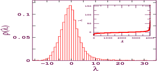
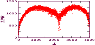
Figure 1: (Color online) Left subfigure plots eigenvalue distribution for the largest connected cluster for the threshold value $th=0.5$. Inset plots eigenvalues in the increasing order. Right subfigure plots IPR as a function of eigen number $i$.

Figure (1) shows IPR as a double humped well. For a network of size $N=4016$, the IPR value for the eigenvectors following RMT prediction would be $\sim 1338$. Based on the eigenvector localization values, the spectra can be divided into two parts, one part with the delocalized eigenvectors having value close to the RMT prediction, and another part which consists the localized eigenvectors. According to RMT, this indicates that the corresponding network has a mixture of random connections yielding the delocalized eigenvectors of the first part, and the structural features corresponding to functional performance leading to the localized second part. In order to get insight to the system dependent properties, we probe localized eigenvectors further. Based on the corresponding eigenvalues, the localized part of the spectra can further be divided into three distinct sub-parts, which we would discuss in detail. The first localized part (A) is associated with the lower eigenvalues regime, the second localized part (B) corresponds to the middle part of the spectra near the zero eigenvalue, and the third localized part (C) corresponds to the eigenstates with larger eigenvalues.

We make following general observations: the eigenvectors belonging to the part (A), in general, have the top contributing nodes with high degrees. The eigenvectors belonging to the part (B) have as few as one or two top contributing nodes. Additionally, these top contributing nodes have as few as one or two degrees. The eigenvectors belonging to the part (C) have top contributing nodes with degree close to the average degree of the network. The eigenvectors belonging to the part (C) do not have distinguished nodes contributing much higher than the rest. Note that for finite dimensional matrix, deviation from randomness determines the localization length of the eigenvectors [32].

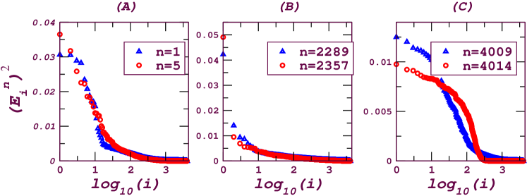
Figure 2: (Color online) Typical behavior of the eigenvector elements from sets (A), (B) and (C). $n$ denotes the eigenstate, and $|E_{i}^{n}|^{2}$ denotes the $ith$ component of the $nth$ eigenvector. Nodes are reordered such that first top contributing node, where contribution is measured by $(E_{i}^{n})^{2}$, gets index $i$ being 1, and last contributing node gets index $i=N$.

Figure (2) plots the square of the eigenvector components for few eigenvectors lying at the bottom of the $IPR$ values. The different nature of eigenvector components in these three parts can clearly be seen. The eigenvectors from set (A) show the localization on approximately ten to twelve nodes, which contribute to the IPR highly. In the reordered nodes, as shown in the Figure (2), contributions from the top ten-twelve nodes decay with the node number, and finally reach to a plateau with very small values of $(E_{i}^{n})^{2}$ for rest of the nodes. The eigenvectors in set (B) are highly localized on few nodes, namely one or two nodes, rest of the nodes lie towards the bottom of the participation measured by $(E_{i}^{n})^{2}$. For the eigenvectors in set (C), the top contributing nodes give approximately same amount of contribution to the participation measure. The top 50 localized eigenvectors, except few, correspond to the eigenstates with the set (A), i.e. with the negative eigenvalues. Note that the eigenstate, corresponding to the largest eigenvalue ($\lambda_{N}$), has exponential decay components, and is not localized to few nodes.

In the following we analyze the top contributing nodes of eigenvectors lying towards the bottom of the IPR table. First, we analyze these nodes under the network theory framework, i.e. based on their degree and position in the network. We use the overlap measure to probe further the structural properties of the nodes. Following this, we would note some of their functional relevance.

The top contributing nodes corresponding to the eigenvectors in the set (B), listed in the Ref. [33], are few, and interestingly one node appears in most of the localized eigenvectors in this set. The first localized eigenvector corresponds to the eigenstate $n=2289$. It has one localized node well separated from the others. This localized node comes at the number $3884$ in the largest connected component. The node lies to the periphery of the network with only one neighbor connected to it. The neighboring node $\mathcal{N}_{3884}\in\{1185\}$ has a very large degree $k_{1185}=145$. The symbol $k_{i}$ denotes the degree of the $i$th node, and $\mathcal{N}_{i}\in\{j_{1},j_{2}....j_{k}\}$ tells that the node $i$ has $k_{i}$ neighbors, namely, node $j_{1}$, node $j_{2}$ and so on.

The next localized eigenvector of set (B) corresponds to the eigenstate $n=2357$, and is localized on two nodes $n=4011$ and $n=4016$. The node number $4011$ is connected to only one node $3038$ with the degree $k_{3038}=19$. The neighbors of $n=3038$ has varying degrees ranging from as low as $1$ to as high as $258$. The overlapping between all the pairs of nodes from the set of $\mathcal{N}_{3038}$ are less or equal to the overlapping in the corresponding random network. Node number $n=4016$ is connected with two other nodes $\mathcal{N}_{4016}\in\{3806,3971\}$ with degrees $30$ and $13$ respectively. Furthermore, these neighbors also do not have any common neighbors.

In order to quantify the overlapping between neighbors of two nodes $i$ and $j$, here we define a measure as,

$$O_{ij}=\frac{2NN_{ij}}{min(NN_{i},NN_{j})}$$ (3)

Where $NN_{i}$ is the number of neighbors of node $i$, and $NN_{ij}$ indicates the number of common neighbors between the nodes $i$ and $j$. Equation 3 measures the fraction of the overlapping neighbors of nodes $i$ and $j$. The value $O_{ij}=0$ corresponds to the case when the nodes $i$ and $j$ do not share any common neighbor, and the value $O_{ij}=1$ corresponds to the situation when all the neighbors of the node $i$ ($j$) are within the set of neighbors of the node $j$ ($i$).

First, we calculate the overlap $O_{ij}$ between all the pairs of nodes $i$ and $j$, where $i$ is the neighboring node $3038$ of the first top contributing node $n=4011$, and the node $j$ being any of the two neighbors $3806,3971$ of the second top contributing node $4016$. The zero value of $O_{ij}$ tells there is no overlapping even between the next to the nearest neighbors of the two top contributing nodes from the first localized eigenvector of set B.

The next two localized eigenvectors of the set B, corresponding to eigenstates $n=2258$ and $n=2282$, also have one localized node $3884$ well separated from the others. The next two eigenvectors are localized on two nodes. Additional to the node number $3884$ which is the top contributing in the previous eigenvectors, there are two other nodes, $3008$ and $4011$, appearing for the eigenvectors corresponding to $n=2298$ and $n=2307$ states respectively.

The localized eigenvectors from set (B) show entirely different features than the eigenvectors belonging to other two sets (A) and (C). The eigenvectors in this set not only have as few as one or two localized nodes, but also these nodes have few number of distinct neighbors.

Figure (3) shows the section of the network consisting of the top contributing nodes, of the localized eigenvectors of set (B). The sub-graph shows all the first (light gray solid circles, cyan) as well as second (light gray dots, orange, to the end of all links) neighbors of these nodes.

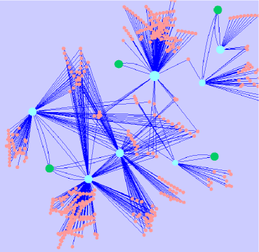
Figure 3: (Color online) Part of the network consisting nodes and neighbors of the nodes corresponding to the set (B), see text for details. The top contributed nodes of the localized eigenvectors of this set are denoted by dark gray solid circles (green). The first neighbors of these nodes are denoted by light gray solid circles (cyan), and the second neighbors are denoted by the light gray dots (orange).

The node number $3008$ (dark gray, green, solid circle towards bottom left) has three neighbors $\mathcal{N}_{3008}\in\{293,302,1821\}$ (light gray, cyan, solid circles connected with the node number $3008$) with large degrees. The first pair of $\mathcal{N}_{3008}$ has 30 % overlapping neighbors whereas other two pairs have $\sim 10\%$ and $\sim 20\%$ overlapping neighbors. Further more, we calculate $O_{ij}$ between all the pairs of $i$ and $j$, where $i$ denotes the neighbors of the first contributing node $n=3884$, and $j$ denotes the neighbors of the second contributing node $n=3008$. The values of $O_{ij}$ for such pairs are close to the value of $O_{ij}$ for the corresponding random network. Similarly, the two top contributing nodes from the eigenvector $E^{(2307)}$ have no next to the nearest common neighbors.

All the above observations suggest the followings: the top contributing nodes in the eigenvector from set (B) are either located on the periphery of the network, or they serve as a bridge to the several loosely separated communities. The top contributing nodes from the same eigenvectors from set (B) belong to the well separated different communities.

The top contributing nodes from set (A), which consists most of the localized eigenvectors, form a separate set for each eigenvector. The top most localized eigenvector corresponds to the minimum eigenvalue ($n=1$). Ten top most contributing nodes for this eigenvector, in serial, are: $99,1101,64,129,245,1243,1238,17,91,226$. All of these nodes have very high degrees, and each node separately form clique of order 10 with its neighbors.

In order to measure the overlapping between the neighbors of the top contributed nodes, we calculate $O_{ij}$ for each pair of the nodes appearing in the top ten list of the different eigenvectors. Figure( 4) plots the overlapping measure $O_{ij}$ for the four most localized eigenvectors. As can be seen from the figure that the values of $O_{ij}$ for the pair of neighbors of the nodes from $E^{(4016)}$ are very high. The overlapping for the pair of nodes beyond ten are inconsistent. Note that the network has the size $N=4016$ and the average degree $<k>\sim 120$, the number of common neighbors for a pair of nodes $i$ and $j$ in a corresponding random network would be of the order of $O_{ij}\sim 0.03$. Figure (4) shows that the overlapping between neighbors of the top ten contributing nodes of eigenvector $E^{(4016)}$ is an order of magnitude larger than that of the corresponding random network. The second most localized eigenvector corresponds to the eigenvalue $\lambda_{5}$. The top ten most contributing nodes again have degree towards the higher side, and they form completely different set than the top contributing nodes in the previous eigenvector. These nodes also form a clique of the order ten. Figure (4) shows that the overlapping $O_{ij}$ between all the pairs of the top ten contributing nodes are very high. Similarly, the third and the fifth most localized eigenvectors also have completely different sets of the top ten contributing nodes. Note that the fourth most localized eigenvector belongs to the set (C). Figure (4) plots $O_{ij}$ for all the pairs of top ten nodes corresponding to the fourth eigenvector as well.

Furthermore, $O_{ij}$ between the nodes from the different top eigenvectors for the set (A) are very low, Figure (4) shows that the overlapping between the different pairs of the nodes from the top four eigenvectors are of the order of the corresponding random network. Note that the degree of these nodes are very high, but they form different subgroups corresponding to each eigenvector, without significant common nodes even with the neighbors of the nodes from the different eigenvectors.

Furthermore, overlapping between the neighbors of the nodes belonging to the different localized eigenvectors from set (A) are few. The values of $O_{ij}$, where $i$ is a node of one eigenvector say $E^{(5)}$ and $j$ is a node from another eigenvector of set A, say $E^{1}$, comes in the bottom of the figure 4. All this suggests that the top contributing nodes in the different eigenvector from set (A) form densely connected community structure within a eigenvector, and which is loosely connected with the nodes from the other eigenvectors.

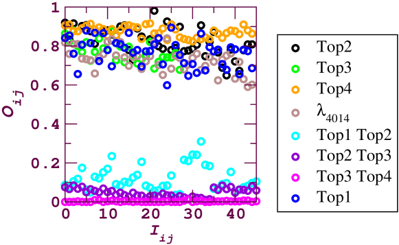
Figure 4: (Color online) Fraction of overlapping neighbors $O_{ij}$ for the pairs of nodes $i$ and $j$. The horizontal label shows the pair index $I_{ij}$, $i$ and $j$ denoting two different nodes, and the vertical axis plots the overlapping between the nodes $i$ and $j$. The overlapping measure for the nodes within the eigenvectors $E^{1},E^{2},E^{3},E^{4}$ and $\lambda_{max}$ are plotted with the different gray shades towards the top of the figure, and the overlapping measure for the pairs of nodes belonging to the different eigenvectors are plotted with different gray shades towards the bottom of the figure.

The first most localized eigenvector in the set (C) corresponds to the $\lambda_{4014}$. Though for this set, not much distinct localized nodes exist, the top ten contributing nodes have their degrees near to the average degree of the network, and these nodes are densely connected with each other. The very high values of $O_{ij}$ in the Figure (4) for $\lambda_{4014}$ indicate that, all the pairs of top contributing nodes share large number of neighbors. These nodes form entirely different set than the top ten nodes of the eigenvector corresponding to the maximum eigenvalue $\lambda_{max}$. The eigenvector corresponding to the maximum eigenvalue comes at the number of $44$ in the terms of localization. Most of the top ten contributing nodes for this eigenvector are same as those for the first localized eigenvector which belongs to the set (A). Contrary to the top nodes in the other eigenvectors of the set (C), the top contributing nodes for $E^{(N)}$ have degree much larger than the average degree of the network. These nodes form a dense community with as high as $\sim 80\%$ of overlapping neighbors between each pair of the nodes. The second most localized eigenvector from this set (C) corresponds to the eigenstate $n=4009$. The average degree of the top ten contributing nodes is close to the average degree of the network, and the nodes show very high overlapping between the neighbors.

4 Conclusion and Discussion

We analyzed spectra of the gene co-expression network of Zebrafish generated for different environmental perturbations. The eigenvalues statistics of the corresponding matrix shows triangular distribution with exponential decay at both the ends. Triangular distribution is one of the known characteristics for scalefree networks. The spacing distribution of the eigenvalues follows GOE statistics of RMT, which indicates that there is sufficient amount of randomness [24] existing in the co-expression network. The eigenvector localization measured by the IPR values shows that the bulk of the spectra follows RMT predictions of the GOE statistics. The remaining part of the spectra which deviates from the RMT predictions carries system dependent information. The later part of the spectra have localized eigenvectors, and is divided into three groups based on the associated eigenvalues. Moreover, top contributing nodes corresponding to the different groups show different structural features. The eigenvectors belonging to the first group (A) has top contributing nodes with high degrees, and are associated with the lower eigenvalues regime. The eigenvectors associated with the second group (B) have top contributing nodes with as few as one or two degrees, and are associated with the zero eigenvalue regime. The eigenvectors from group (C) lie towards the largest eigenvalue, and have top contributing nodes with degrees close to the average degree of the network. Most of the top localized eigenvectors belong to the part (A), i.e. correspond to the lower eigenvalues regime. According to the RMT, the localized eigenvectors distinguish ’genuine correlations from apparent correlations’ [15] which, in terms of the gene co-expression networks, can be interpreted as random correlations between the genes and functionally important correlations between the genes. The corresponding matrix is not random, and hence leads to the localization of some of the the eigenvectors. The top contributing nodes in the localized eigenvalues may have important structural and functional roles.

In order to probe the structural relevance of the top contributing nodes we define overlap measure. For the set (B), overlapping measure shows that the top contributing nodes lie towards the periphery of the network. Additionally, based on the overlap measure for the neighbors of the top contributing nodes from localized eigenvectors, we see that these nodes belong to the different regions of the network with a small overlapping between even the next to the nearest neighbors. The largest overlap in these pairs is those of the corresponding random networks. These observations suggest that for the set (B), the top contributing nodes belonging to same eigenvectors lie either near to the periphery, or belong to the different parts of the networks.

For the set (A), the top contributing nodes of a eigenvector have very high values of the overlap measure, infact for some of the localized eigenvectors these nodes are part of the clique of the order ten. Furthermore, the top contributing nodes from the different localized eigenvectors lie well separated from each other. All the observations for set (A) indicate that the top contributing nodes in different eigenvectors form separate community structure; these communities are densely connected within, and are loosely connected with each other.

The top contributing nodes from the set (C) do not show any noticeable structural features, except the fact that, the nodes from each localized eigenvector form densely connected set though they have less number of neighbors, equal to the average degree of the network.

Description in the Ref. [33] suggests that most of the genes in the localized sets, which are functionally related or are members of pathways leading to similar diseases, are basically clustered in one set. The exceptional cases, however, may indicate that although these genes were identified in the same set, having different function altogether, could have similar protein expression patterns that are regulated by similar transcriptional cues in similar developmental domains, like that of the other members in that particular set. Though the biological interpretation drawn in the letter is at a preliminary stage, the analysis presented here shows the applicability and the usefulness of random matrix theory to pick out set of nodes (genes) from a large number of interacting nodes (genes), which were not detected based on existing structural measures. Identification of genes that are significantly responsible for diverse toxicological perturbations is important in order to develop a future chip, that can be used for detection of pollutants and diagnosis of diseases. Future directions would involve hand in hand experiments and theoretical investigations to make direct relation between cause such as environmental perturbations and gene or set of genes affected.

5 Acknowledgment

The microarrays works were supported by Environment and Water Industry Grant of Singapore. CYU and LZ are currently supported by grant MOE2009-T2-2-064. SJ acknowledges DST grant SR/FTP/PS-067/2011 for the financial support.

References

- [1] López-Maury L. et. al., Nat. Genet. 9 583 (2008).
- [2] Gasch A. P. et. al., Mol. Biol. Cell 11 4241 (2000).
- [3] Maslov S. and Sneppen K., Science 296, 910 (2002); Hishigaki H. et. al. Yeast 18 523 (2001).
- [4] Liang W. S. et. al., Physiol Genomics 28 (3), 311 (2007); W. S. Liang et. al., Proc Natl Acad Sci U S A, 105 4441 (2008).
- [5] Barabási A. -L. and Albert R., Science 286, 509 (1999).
- [6] Strogatz S. H., Nature 410, 268 (2001).
- [7] Albert R. and Barabási A. -L., Rev. Mod. Phys. 74, 47 (2002) ; Boccaletti S. et. al., Phys. Rep. 424, 175 (2006).
- [8] Ung C. Y. et. al., PloS One 6 27819 (2011).
- [9] Stuart J. M. et. al., Science 302 249 (2003).
- [10] Grunwald D. J. and Eisen J. S., Nat Rev Genet, 3 717 (2002).
- [11] Shin J. T. and Fishman M. C., Annu Rev Genomics Human Genet 3 311 (2002).
- [12] Spitsbergen J. M. and Kent M. L., Toxicol Pathol 31 62 (2003)
- [13] Mehta M. L., Random Matrices, 2nd ed. (Academic Press, New York, 1991).
- [14] Guhr T. et. al., Phys. Rep. 299, 189 (1998).
- [15] Pleron V. et. al., Phys. Rev. Lett. 83, 1471 (1999).
- [16] Seba P., Phys. Rev. Lett. 91, 198104 (2003).
- [17] Santhanam M. S. and Patra P. K., Phys. Rev. E 64,016102 (2001).
- [18] Bandyopadhyay J. N. and Jalan S., Phys. Rev. E, 76, 026109 (2007); Jalan S. and Bandyopadhyay J. N., Phys. Rev. E, 76, 046107 (2007).
- [19] de Carvalho J. X. et. al., Phys. Rev. E 79 056222 (2009).
- [20] Jalan S., Phys. Rev. E 80, 046101 (2009).
- [21] Potestio R. et. al., Phys. Rev. Lett. 103 268101 (2009).
- [22] http://www.ncbi.nlm.nih.gov/geo/
- [23] Jalan S. et. al Phys. Rev. E 81, 046118 (2010).
- [24] Jalan S. and Bandyopadhyay J. N., EPL 87 48010 (2009).
- [25] Analysis of Microarrays Data - A Network-Based Approach edited by M. Dehmer and F. Emmert-Streib (Wiley-VCH, Weinheim, 2008).
- [26] Kerr M. and Churchill G. A., Proc. Natl. Acad. Sci. of the U.S.A., 98 8961 (2001); Kerr M. et. al., Journal of Computational Biology, 7 819, (2000).
- [27] If instead of the bootstrapping approach we use just the sample correlation coefficient, a larger set of links would be present which would contain genes having very large bootstrap confidence intervals.
- [28] Zyczkowski K., chapter in Quantum chaos, edited by H. A. Cerdeira, R. Ramaswami, M. C. Gutzwiller and G. Casati, (World Scientific, 1991).
- [29] F. Haake and K. Źyczkowski, Phys. Rev. E 42 1012 (1990).
- [30] Zhou X. et. al., Proc. Natl. Acad. Sci. 99, 12783 (2002); Smet D. et. al., Bioinformatics 18 735 (2002).
- [31] F. Luo et. al., Bioinformatics 8 299 (2007).
- [32] F. Evers and A. D. Mirlin, Rev. Mod. Phys. 80 1355 (2008).
- [33] See supplementary material at http://people.iiti.ac.in/sarika/Supplement.pdf