Model Independent Early Expansion History and Dark Energy

Abstract

We examine model independent constraints on the high redshift and prerecombination expansion history from cosmic microwave background observations, using a combination of principal component analysis and other techniques. This can be translated to model independent limits on early dark energy and the number of relativistic species $N_{\rm eff}$. Models such as scaling (Doran-Robbers), dark radiation ($\Delta N_{\rm eff}$), and barotropic aether fall into distinct regions of eigenspace and can be easily distinguished from each other. Incoming CMB data will map the expansion history from $z=0$–$10^{5}$, achieving subpercent precision around recombination, and enable determination of the amount of early dark energy and valuable guidance to its nature.

I Introduction

The expansion history of the universe is a fundamental property of cosmology, reflecting the energy density constituents and their evolution. Yet remarkably little is known in detail about it, other than in a coarse grained average. For redshifts between 3000 and $10^{9}$, the universe was mostly radiation dominated, for redshifts between 3000 and $\sim 1$ it was mostly matter dominated, but excursions are possible – in the effective number of relativistic species $N_{\rm eff}$ say, or even temporary breakdown of such domination – and the level of subdominant components is not well constrained. Only around the epoch of primordial nucleosynthesis and of recombination is the expansion rate (Hubble parameter) better constrained, but even there at the $\sim 5\%$ level averaged over the epoch kaplinghat ; zahn .

Given the importance of the expansion history, and the improvement in cosmic microwave background (CMB) data, we investigate what constraints can be placed on it in a model independent way, i.e. other than fitting for a deviation of a particular functional form such as extra $N_{\rm eff}$ or a specific dark energy model. This would fill in a vast range of cosmic expansion where almost no precise constraints have been placed. That is, an error band for the Hubble parameter $H(z)$ at $z>1000$ should be a staple of cosmology textbooks, and yet does not exist.

The early expansion history has an important bearing on understanding the nature of dark energy as well, the question of persistence of dark energy. For a cosmological constant $\Lambda$, the dark energy density contributed at recombination is $\Omega_{\Lambda}\approx 10^{-9}$, while the current upper limit from data is above $10^{-2}$. This gives substantial unexplored territory. Moreover, the current constraints use a specific functional form for the dark energy evolution (usually the Doran-Robbers form dorrob ), but other models could lead to significantly different limits rdof . Thus, model independent limits on early dark energy are needed. Physics origins for early dark energy can be quite diverse, e.g. from dilaton models (as in some string theories) to k-essence (noncanonical kinetic field theories) to dark radiation (as in some higher dimension theories) cope . Establishing whether CMB observations could distinguish these classes is another important question.

Improvement of CMB data recently by higher resolution observations extending the temperature power spectrum to multipoles $\ell\approx 3000$ by the Atacama Cosmology Telescope (ACT act ) and South Pole Telescope (SPT spt ) gives valuable leverage since higher multipoles are sensitive to modes crossing the cosmological horizon at earlier times. This advance was used in linsmith to rule out in a model independent manner the presence of any epoch of cosmic acceleration between $z\approx 2$ and $10^{5}$ (supplementing the limits from growth of structure post-recombination in unique ). Upcoming Planck and ground based polarization experiment data will also map out the polarization power spectra, giving additional constraints.

To carry out a model independent analysis of the early expansion history, we use a combination of redshift binning and principal component analysis. In Sec. II we lay out the methodology for describing arbitrary $H(z)$. Analyzing the results in Sec. III, we identify the redshifts ranges where the CMB observations are most sensitive to expansion variations. We project three classes of models representing different physical origins onto the eigenmodes to explore the discriminating power of the data in Sec. IV. In Sec. V we discuss the results and future prospects.

II Expansion History

The expansion Friedmann equation directly relates the expansion rate of the universe, or Hubble parameter, to the energy density constituents,

$$H^{2}(a)=\frac{8\pi G}{3}\sum\rho_{i}(a)\ ,$$ (1)

where we neglect curvature (from a theoretical prior for flatness and because we mostly treat high redshift where it would be negligible). At high redshift the canonical expectation is that the universe is matter or radiation dominated, so we write

$$H^{2}(a) = \frac{8\pi G}{3}\,[\rho_{m}(a)+\rho_{r}(a)+\rho_{\Lambda}]+\delta H^{2}(a)$$ (2)

$$= H^{2}_{\rm fid}+\delta H^{2}(a)$$ (3)

$$= H^{2}_{\rm fid}\,[1+\delta(a)]\ .$$ (4)

Deviations $\delta(a)$ to the fiducial expansion rate can also be interpreted as an effective dark energy density differing from that of the cosmological constant, with

$$\rho_{de}(a)=\rho_{\Lambda}+\frac{3H^{2}_{\rm fid}}{8\pi G}\,\delta\ .$$ (5)

We can write the dark energy density evolution as

$$\rho_{de}(a) = \rho_{de,0}\,f(a)=\rho_{\Lambda}\,f(a)$$ (6)

$$f(a) = 1+\left(1+\frac{\rho_{bg}}{\rho_{\Lambda}}\right)\,\delta\ ,$$ (7)

where $\rho_{bg}$ is the background energy density excepting dark energy, i.e. usually the dominant component, matter or radiation. More simply, the fraction of critical density contributed by the effective dark energy is

$$\Omega_{de}(a)=\frac{8\pi G\rho_{\Lambda}}{3H^{2}_{\rm fid}\,(1+\delta)}+\frac{\delta}{1+\delta}=\frac{\Omega_{\Lambda}(a)+\delta}{1+\delta}\ .$$ (8)

We can readily see that at high redshift we obtain a fractional early dark energy density contribution of approximately $\delta(a)$, for $\Omega_{\Lambda}(a)\ll\delta\ll 1$. During epochs when $\delta$ is constant, this is a constant fractional contribution.

Our goal is to analyze constraints on the variations $\delta(a)$ from the canonical model with $\delta=0$. We begin by writing $\delta(a)$ as a linear combination in an orthogonal bin basis,

$$\delta(a)=\sum\beta_{i}b_{i}(a)\ ,$$ (9)

where $b_{i}(a)$ is a tophat of amplitude 1 over a given range of scale factor $a$, and 0 otherwise. That is, the Hubble parameter deviations $\delta(a)$ are given as a linear combination of piecewise constant values. We can then constrain $H(a)$ in bins of $a$, a model independent description. The bin basis is also the standard first step in principal component analysis (see, e.g., hutstar ), as we will pursue in the next section. We choose $N$ bins per decade of scale factor over the range of $\log a=[-5,0]$, beginning with $N=20$.

Since we are interested in the expansion history we deal directly with the Hubble parameter (or effective dark energy density). Treating bins of the dark energy equation of state, or pressure to density, ratio $w(z)$ would have some drawbacks here. Most severe is that to obtain $H(z)$ one must integrate $w(z^{\prime})$ over all redshifts from zero to $z$. This makes it difficult to explore the early expansion history in a model independent manner. Moreover, the instantaneous $w(z)$ is not fully informative: during matter domination, for example, any level of dark energy density from $\Omega_{de}=10^{-9}$ to $10^{-2}$ or whatever that scales as the matter has $w=0$. Thus we aim to derive constraints directly on variations in $H(z)$, and consider the interpretation of these as a further step.

The expansion history directly feeds into the CMB power spectra, through changing the distance scales, e.g. of the sound horizon or damping scale, and the relation of multipole $\ell$ (or angular scale $\theta$) to wavenumber $k=\ell/\eta(z)$, where $\eta$ is the conformal distance. It also affects the decoupling of photons from baryons and the growth of perturbations in both.

The treatment of perturbations requires some attention. The description of the cosmic expansion gives the evolution of the homogeneous background, but consistency of the field equations requires consideration of perturbations in all components of energy density. Unless the deviation in $H(z)$ is interpreted purely in terms of a cosmological constant (which indeed is purely homogeneous), spatial perturbations have to be accounted for, at least formally and generally in actual practice. The perturbation evolution equations for the additional energy density involve the quantities $w(z)$, $w^{\prime}(z)=dw/d\ln a$, the initial conditions on the density perturbation, and the sound speed of the effective fluid $c_{s}(z)$. (One could also add a viscous sound speed or anisotropic stresses, see hu1998 .)

The first three of these are fairly straightforward. For any deviation $\delta(a)$ one can define an effective equation of state

$$w = -1-\frac{1}{3}\frac{d\ln\rho_{de}}{d\ln a}$$ (10)

$$= -1-\frac{a}{3[1+\delta(1+\rho_{bg}/\rho_{\Lambda})]}\left[\left(1+\frac{\rho_{bg}}{\rho_{\Lambda}}\right)\frac{d\delta}{da}+\frac{\delta}{\rho_{\Lambda}}\frac{d\rho_{bg}}{da}\right]$$ (11)

$$\approx w_{bg}-\frac{1}{3}\frac{d\ln\delta}{d\ln a}\ ,$$ (12)

where the last line holds when $\rho_{\Lambda}$ gives negligible contribution to the effective dark energy density. One can take a further derivative to obtain $w^{\prime}$. Initial conditions are usually taken as adiabatic and stresses are taken to vanish. However, one does have to specify the sound speed. If one interprets the extra energy density as arising from quintessence, i.e. a minimally coupled, canonical scalar field, then $c_{s}=1$. In general, the necessary inclusion of perturbations in whatever is the origin of the deviations in the expansion history prevents a purely model independent treatment – one has to make some assumptions about the physics. Here we fix $c_{s}$ to that for the particular cases we consider, but in future work we will fit for it.

We modified CAMB camb to allow a general $H(z)$, with the $w(z)$ that goes along with this. We then solve the coupled background evolution, and photon, matter, and effective dark energy perturbations equations to obtain the CMB power spectra. For evaluating binned $H(z)$ models, using the orthogonal bin basis introduced in Eq. (9), we slightly smooth the bin edges, using a Gaussian smoothing of width $0.075$ times the bin width, to prevent infinite derivatives. We extensively test convergence and numerical stability of the results (also see linsmith where this procedure was found to be robust).

Figure 1 shows the bins in log scale factor (20 bins per decade) and the conversion to multipole space (overlaid with the CMB temperature power spectrum) by $\ell\approx\eta_{0}/\eta(a)$, which approximately relates a given wavenumber $k\approx\ell/\eta_{0}$ to the time it entered the horizon. Note that a uniform binning in $\log a$, which is the expected characteristic scale for physical variations in the expansion, is not uniform in multipole space.

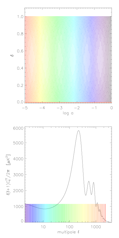
Figure 1: [Top] The bin basis for expansion variations $\delta(a_{i})$ is plotted vs $\log a$. [Bottom] The scale factors $a_{i}$ of the center of each bin in the top panel (with matching colors) are approximately mapped into multipoles by $\ell\approx\eta_{0}/\eta(a_{i})$, with the CMB temperature power spectrum overplotted. (Amplitudes of the colored lines are arbitrary.)

To place constraints on allowed deviations $\delta(a)$ we carry out a Fisher matrix calculation. The Fisher matrix elements are given by

$$F_{ij}=\sum_{l}\sum_{X,Y}\frac{\partial{C_{Xl}}}{\partial{p_{i}}}(COV_{l})^{-1}_{XY}\frac{\partial{C_{Yl}}}{\partial{p_{j}}}$$ (13)

where $X,Y$ is any combination of the CMB temperature power spectrum (T), E-mode polarization power spectrum (E), and temperature-polarization cross power spectrum (TE). The covariance matrix $COV$ is given by the measurement uncertainties of the CMB observations; we adopt the characteristics of the Planck satellite experiment planck . The parameter set $\{p_{i}\}$ includes the usual cosmological parameters – the physical baryon density $\Omega_{b}h^{2}$, physical cold dark matter density $\Omega_{c}h^{2}$, total present matter density $\Omega_{m}$ (the present Hubble constant $h$ is a derived quantity), primordial scalar perturbation power law index $n_{s}$, optical depth $\tau$, and present amplitude of mass fluctuations $\sigma_{8}$ – and the $N_{\rm bin}$ expansion variation parameters $\delta(a_{i})$. The uncertainties on each $\delta(a_{i})$ are given by the (square root of the) respective diagonal element of the inverse of the Fisher matrix.

Figure 2 shows the sensitivity $\sqrt{F_{ii,\ell}}$ of the weighted combination of CMB power spectra (T, E, TE) to the expansion deviations in each redshift bin for each multipole. Sensitivity peaks around the acoustic peaks and is reduced at low multipoles due to cosmic variance and at high multipoles due to the finite resolution from the instrument beam size. Since the polarization power spectrum is out of phase with the temperature power spectrum, dips in the temperature sensitivity are filled in by polarization information.

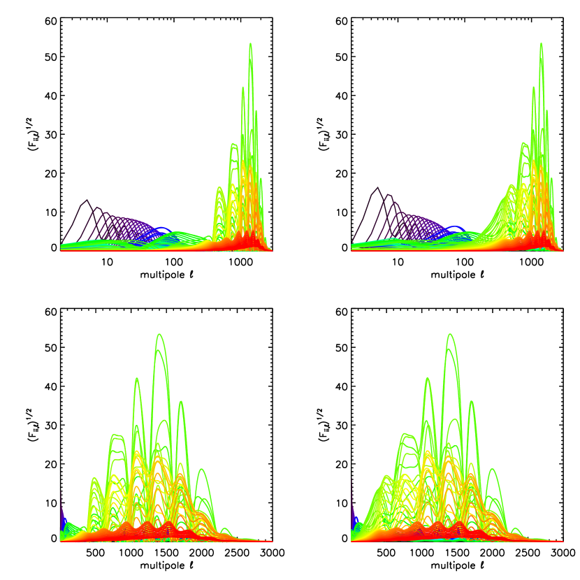
Figure 2: The fractional Fisher sensitivities, $\sqrt{F_{ii,\ell}}$, to the expansion variations $\delta(a_{i})$ in each bin, color coded as in Fig. 1, are plotted vs multipole. The top panels use log scale in multipole, the bottom panels a linear scale to highlight different regions. The left panels are for the temperature power spectrum only, while the right panels use the variance weighted sum of the T, E, and TE power spectra entering the Fisher information matrix. Polarization information fills in the sensitivity gaps due to the acoustic troughs.

Figure 3 shows the actual Fisher and covariance submatrices corresponding to the expansion bin parameters (marginalized over other parameters in the case of the covariance matrix). First, we notice the maximum of the information content is near decoupling ($\log a\approx-3$), as expected. Earlier times, $\log a<-4$, map to multipoles on the damping tail and so have less leverage, while recent times, $\log a>-3$, are on the Sachs-Wolfe plateau and again have limited information. The Fisher matrix is not diagonal because expansion deviations affect all later times, e.g. perturbation evolution once the wavemode is within horizon and integral quantities such as the sound horizon. This will be one of the motivating factors for carrying out principal component analysis (PCA) in Sec. III. The covariance matrix (inverse of the Fisher matrix), however, has a more diagonal structure, and so bins can be a useful parameter set if carefully chosen (see Sec. V).

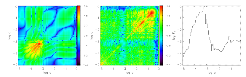
Figure 3: The Fisher information submatrix (left) corresponding to the expansion variation parameters $\delta(a_{i})$ is plotted with redder shades representing larger absolute values (more information). The color bar gives the log of the absolute value of elements. The covariance matrix (middle), marginalized over other cosmological parameters, follows the same color scheme, so the best determined parameters (smallest errors) are bluest. Diagonal elements of the Fisher matrix (right), as a fraction of the largest diagonal element, quantify for which redshifts the CMB data is most sensitive to the expansion history. The bump at $\log a\approx-1.1$ reflects reionization.

Most importantly, Figure 4 shows the constraints on the expansion history

$$\frac{\sigma(H)}{H_{\rm fid}}=\frac{\sigma(\delta)}{2\sqrt{1+\delta}}\ ,$$ (14)

i.e. the fractional uncertainty on $H(a)$ due to deviations $\delta$, marginalized over the other cosmological parameters. This is the “textbook” plot, showing the state of our knowledge of the early expansion history of the universe when given CMB data of Planck sensitivity. The constraints depend on what bandwidth we wish to constrain the expansion history: the top curve shows 10 bins per decade, the bottom curve 2 bins per decade. One can trade off sensitivity to fine features vs overall level of constraints. With 10 bins per decade one can achieve percent level constraints on $H^{2}(a)$ near decoupling, while with 2 bins per decade one obtains subpercent constraints over more than two decades in scale factor. The relation between 10 bins and 2 bins is not simply a $\sqrt{5}$ scaling due to correlations between bins (the offdiagonal elements of the covariance matrix), and the lowest redshift bin is particularly affected by covariance with the other cosmological parameters.

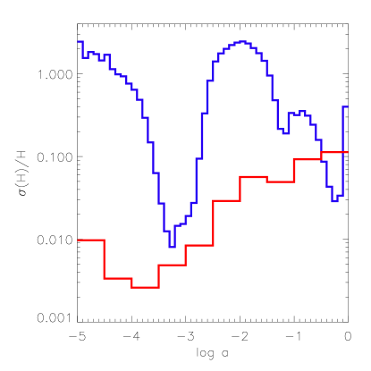
Figure 4: The fractional precision with which the expansion history can be determined by projected Planck CMB data is plotted vs scale factor, for two different bandwidths. The top (bottom) curve is for 10 (2) bins per decade in scale factor. Subpercent precision can be achieved around decoupling but large swaths of the cosmic history will remain unknown.

III Principal Components of Expansion

Expansion deviations at some redshifts may have substantially the same consequence for the observables as deviations at some other redshift, or deviations may be correlated in such a way that only the difference between them is important. This leads to the idea of compressing the 100 bins between $\log a=[-5,0]$, or at least the information contained in them, into fewer variables. One might for example speculate that the major effect of expansion deviations for $a>10^{-3}$ comes from shifting the distance to CMB last scattering, and whether the variation occurs at $a=0.01$ or $a=0.1$ is less crucial.

Principal component analysis (PCA) can provide an efficient way to compress the influence on the observables. For some uses probing dark energy and the CMB, see for example huoka ; hutstar ; leach ; reion ; tobin ; dvor (and dark matter and the CMB in fink ). By diagonalizing the Fisher matrix we can find its eigenvectors that best summarize the sensitivity of the observations to the expansion deviations. We can then transform the bin basis to an orthogonal eigenmode basis of principal components (PCs), writing

$$\delta(a)=\sum m_{i}\,e_{i}(a)\ ,$$ (15)

where $m_{i}$ is the amplitude of mode $i$ and $e_{i}(a)$ is the eigenvector. Since the modes are orthogonal, the errors $\sigma_{i}\equiv\sigma(m_{i})$ on the amplitudes are uncorrelated. Using the entire set of bins or the entire set of PCs is equivalent, but using only a few PCs with the highest eigenvalues (smallest $\sigma_{i}$) in general allows one to approximate the full set more accurately than the same number of bins. That is, the information can be compressed.

Figure 5 illustrates some of the PCs for the CMB Fisher matrix, ordered from highest to lowest eigenvalues (best to worst determined). Note that as expected most of the activity in the first PCs is prerecombination, associated with the acoustic peaks. In modes 7-10, there is some low redshift action coming primarily from the integrated distance to last scattering and the reionization epoch. Higher PC modes tend to be more oscillatory (essentially high derivatives of the expansion behavior) and localized.

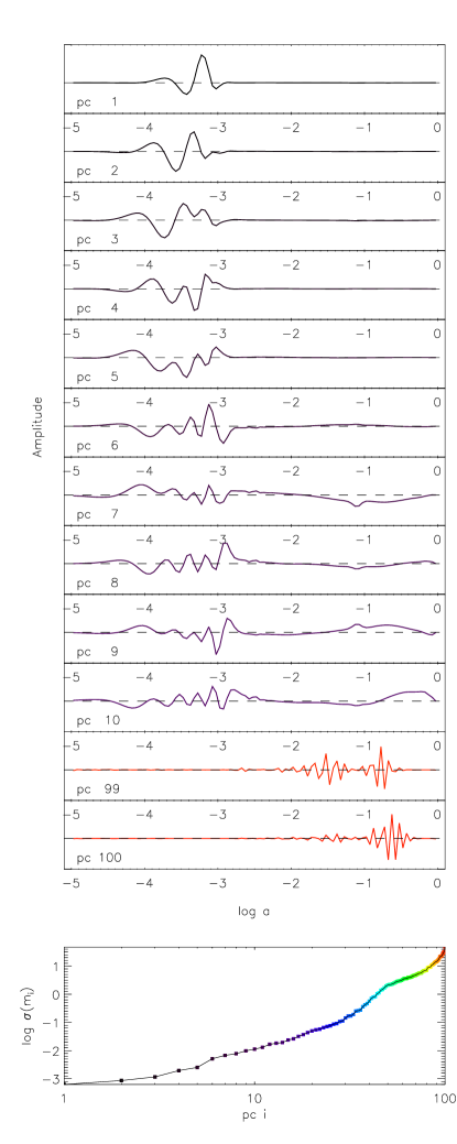
Figure 5: Principal components of the CMB observational sensitivity to expansion history are plotted vs $\log a$, for the first 10 and last 2 modes. The bottom plot shows the $\sigma_{i}$ for all modes.

By taking the cumulative sum of the eigenvalues, we find that the first 7 PCs contain 99% of the variance. That is, $\sum_{1}^{7}\sigma_{i}^{-2}/\sum_{1}^{100}\sigma_{i}^{-2}=0.99$. This means that the great majority of expansion behaviors, as far as their observational detectability is concerned, can be described with just 7 parameters $m_{1},\dots m_{7}$.

It is convenient to normalize the PCs such that $\sum_{n}e_{i}(a_{n})e_{j}(a_{n})=\delta_{ij}$, where $\delta_{ij}$ here is the Kronecker delta, and then the mode coefficients $m_{i}$ give the amplitudes for a given model of expansion history deviation,

$$m_{i}=\sum_{n}\delta(a_{n})e_{i}(a_{n})\ ,$$ (16)

where $a_{n}$ denotes the bin centers. For many narrow bins the sum can be converted to an integral. The amplitudes $m_{i}$ only have meaning when discussing a specific model; note the canonical model $\Lambda$CDM has all $m_{i}=0$. Since the mode amplitude $m_{i}$ has no a priori magnitude, we do not know whether its uncertainty $\sigma_{i}=0.01$, say, is a small or large number. We can compare $\sigma_{i}$’s to each other (but if the $m_{i}$ are 0 this is irrelevant), or for a specific model we can form a signal to noise ratio for a mode,

$$(S/N)_{i}=m_{i}/\sigma_{i}\ .$$ (17)

If $(S/N)_{i}\ll 1$, then it does not matter if $\sigma_{i}$ looks small, the mode cannot be well measured. Thus caution must be used in interpreting PCA (for more details see tobin ; beingpc ).

Although PCA certainly compresses the information content into fewer parameters, the number of PCs required to describe arbitrary expansion histories is still large for the purposes of, say, Monte Carlo simulations. We can therefore use PCA instead as a guide in two ways: to examine the ability to discriminate among different classes of models for the expansion deviation, and to indicate which regions in $a$ show the most sensitivity to deviations and hence which of the original bins are most useful. These are treated respectively in Sec. IV and Sec. V.

IV Comparing Early Dark Energy Models

While we wish to concentrate, as much as possible, on a model independent approach to constraining the expansion history, it is useful to make contact with various classes of models to make sure that important behaviors are captured. In broad strokes, one can consider cases where the expansion deviations decline at times earlier than recombination, increase at earlier times, or remain constant. This can be translated into early dark energy models that contribute a lower fraction of the total energy density in radiation vs matter domination, a higher fraction, or a constant fraction. This tilt of the expansion rate can be an important discriminant, somewhat analogous to the tilt of the primordial power spectrum for inflation.

Early dark energy models have been proposed with each of these behaviors. Examples of the three classes respectively are 1) Barotropic dark energy with sound speed $c_{s}^{2}=0$ linscher , sometimes called aether models, 2) Barotropic dark energy with sound speed $c_{s}^{2}=1/3$ linscher , sometimes called dark radiation, and 3) Scaling dark energy such as the commonly used Doran-Robbers model with $c_{s}^{2}=1$ dorrob .

Barotropic models have $w(a)$, $\rho_{de}(a)$, and hence $\delta(a)$, all determined by $c_{s}^{2}(a)$. The dynamics is given by linscher

$$w^{\prime}=-3(1+w)(c_{s}^{2}-w)\ ,$$ (18)

with solution for constant $c_{s}$ of

$$w(a)=\frac{c_{s}^{2}Ba^{-3(1+c_{s}^{2})}-1}{Ba^{-3(1+c_{s}^{2})}+1}\ ,$$ (19)

where $B=(1+w_{0})/(c_{s}^{2}-w_{0})$. For the $c_{s}^{2}=0$ aether model,

$$\rho_{ae}(a) = \rho_{\infty}+\Omega_{e}\rho_{m,0}a^{-3}$$ (20)

$$\delta_{ae}(a) = \Omega_{e}\,\frac{\Omega_{m}(a^{-3}-1)}{\Omega_{m}(a^{-3}-1)+\Omega_{r}a^{-4}+1}$$ (21)

$$\rho_{\infty}/\rho_{crit,0} = 1-\Omega_{m}(1+\Omega_{e})=(-w_{0})(1-\Omega_{m})$$ (22)

$$w_{0} = -1+\frac{\Omega_{e}\Omega_{m}}{1-\Omega_{m}}\ ,$$ (23)

where during matter domination the dark energy contributed a constant fractional density $\Omega_{e}$, but this declines at earlier times as radiation becomes important.

For the $c_{s}^{2}=1/3$ dark radiation model,

$$\rho_{dr}(a) = \rho_{\infty}+\Omega_{e}\rho_{r,0}a^{-4}$$ (24)

$$\delta_{dr}(a) = \Omega_{e}\,\frac{\Omega_{r}(a^{-4}-1)}{\Omega_{r}(a^{-4}-1)+\Omega_{m}(a^{-3}-1)+1}$$ (25)

$$\rho_{\infty}/\rho_{crit,0} \approx 1-\Omega_{m}$$ (26)

$$w_{0} \approx -1\ ,$$ (27)

where during radiation domination the dark energy contributed a constant fractional density $\Omega_{e}$, but this declines at later times as matter becomes important.

The most commonly used early dark energy is the Doran-Robbers form dorrob ,

$$\Omega_{de}(a)=\frac{1-\Omega_{m}-\Omega_{e}(1-a^{-3w_{0}})}{1-\Omega_{m}(1-a^{3w_{0}})}+\Omega_{e}(1-a^{-3w_{0}})\ ,$$ (28)

where during both matter and radiation domination the dark energy contributed a constant fractional density $\Omega_{e}$. The sound speed is conventionally taken to be $c_{s}^{2}=1$.

Thus the three models we consider have expansion history deviations with complementary behaviors: rising, falling, and constant. This range should give a good indication of how PCA can characterize the expansion, while also having physical motivations. Of the physics origins mentioned in the Introduction, some string theories give Doran-Robbers behavior, some noncanonical kinetic fields give aether behavior, and some higher dimension theories give dark radiation.

Once we calculate the $m_{i}$ for a model through Eq. (16), we have a better indication of the importance of a PC mode through the signal to noise criterion of Eq. (17) – recall that the $\sigma_{i}$ alone say little about whether the mode is relevant. To choose the number of modes to keep in describing a model, we can simply impose a $S/N$ cutoff, or ask that the cumulative $S/N$ of the modes kept be above some fraction, e.g. 95% of the total $S/N$ from all modes.

Another indicator is the statistical risk, or mean squared error. This takes into account that more modes decrease the bias from the true model, but increase the accumulated variance in $\delta$. The risk $R_{N}$ is

$$R_{N} = \sqrt{b_{N}^{2}+\sigma_{N}^{2}}$$ (29)

$$b_{N}^{2} = \sum_{n}[\delta^{\rm model}(a_{n})-\delta^{N\,{\rm PCs}}(a_{n})]^{2}$$ (30)

$$\sigma_{N}^{2} = \sum_{n}\sum_{i=1}^{N}\sigma_{i}^{2}e_{i}^{2}(a_{n})\ .$$ (31)

One could choose to keep that number $N$ PCs where $R_{N}$ is minimized.

Figure 6 shows for each of the three models the approximation to $\delta(a)$ as more PCs are added, the values $m_{i}$, and the cumulative $S/N$ and risk as a function of number of PCs used. In general we find the risk requires more PCs than the $S/N$ criterion; this makes sense since $S/N$ concentrates on those PCs fitting the observable (CMB power spectra) while risk attempts to fit the unobservable expansion deviation. Another drawback to risk is that it does not scale with the amplitude of the modes, i.e. while $S/N$ increases linearly with $\Omega_{e}$, the bias term in the risk scales but the variance does not, so the risk is weighted unevenly depending on deviation amplitude.

For the dark radiation, aether, and Doran-Robbers models, respectively, we should keep the first 6, 7, and 5 PCs according to $S/N$, and 10, 14, and 15 PCs according to risk. However, we note that this is if we keep the PCs in order according to $\sigma_{i}$. If we choose the highest $S/N$ modes individually, we only require 4, 3, and 3 modes to attain 95% of the full $S/N$ (but this requires knowing the correct model, or assuming a given set of models).

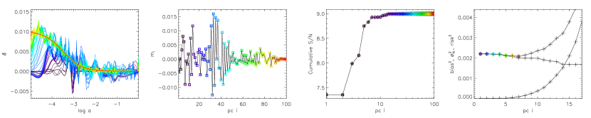
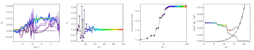
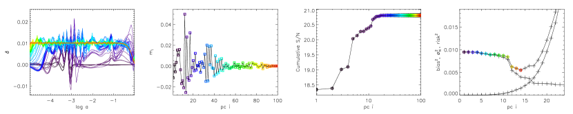
Figure 6: Three models of early dark energy are analyzed – dark radiation (top row), aether (middle row), and Doran-Robbers (bottom row) – with different recombination era behaviors. The leftmost column shows $\delta(a)$ built up out of PCs, with the thick red line giving the exact model. The second column gives the PC amplitudes $m_{i}$ and the third column shows the cumulative $S/N$, summing Eq. (17) over the first $i$ PCs in quadrature. The rightmost column shows the bias squared (falling curve), variance (rising curve), and risk squared (top curve) when including the first $i$ PCs. One might choose to keep those PCs that either give the largest jumps in $S/N$, or all those up to the minimum in the risk curve.

Let us examine these models in more detail. Figure 7 shows how these models are well separated in eigenmode coefficient space. Considerable discriminating power occurs using modes 1 and 7, for example, with the separations between the three models many times the uncertainties $\sigma_{i}$. From the shape of the modes in Fig. 5, we can see that mode 1 is roughly measuring the amplitude of the expansion deviation at recombination, and whether it is increasing or decreasing (thus distinguishing all three models), and mode 7 is sensitive to more recent deviations such as occurring in Doran-Robber and aether, but not dark radiation, cases. Thus these two modes together are adept at distinguishing between the rising, falling, and constant deviation classes of expansion history, and early vs late deviations.

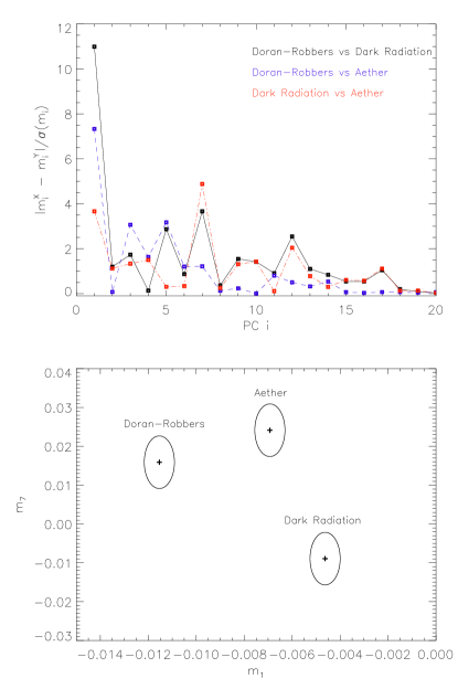
Figure 7: (Top) Differences between each PC amplitude $m_{i}$ are shown for pairs $(X,Y)$ of early dark energy models, with solid curves comparing Doran-Robbers to dark radiation, dashed Doran-Robbers to aether, and dot-dashed dark radiation to aether. The highest peaks indicate the modes with strong discriminating power. (Bottom) Amplitudes of modes 1 and 7 are plotted for the three models, with the +’s indicating the values $m_{i}$ and the ellipses showing the uncertainties $\sigma_{i}$. These two modes can clearly distinguish between each of the three models.

We emphasize that the PCs are really telling us about fits to the observable power spectra and not reconstruction of the expansion deviation in a fine grained sense. While Fig. 6 shows that $\sim 50$ PCs are needed to model $\delta(a)$ well for these example, Fig. 8 demonstrates that only $\sim 10$ PCs are needed to give accurate agreement in $C_{\ell}$. Figure 8 shows the residual of the CMB temperature power spectrum from the sum of the first $N$ PCs (in $S/N$ ordering, and also shown in $\sigma_{i}$ ordering for the aether model) relative to the true model for the three models, as well as the $\chi^{2}$ summed over multipoles, and the reconstructed expansion history. Although the reconstructed expansion history may only agree over certain ranges of $a$, this can still give excellent agreement for the observables as the power spectra are not equally sensitive to all scale factors.

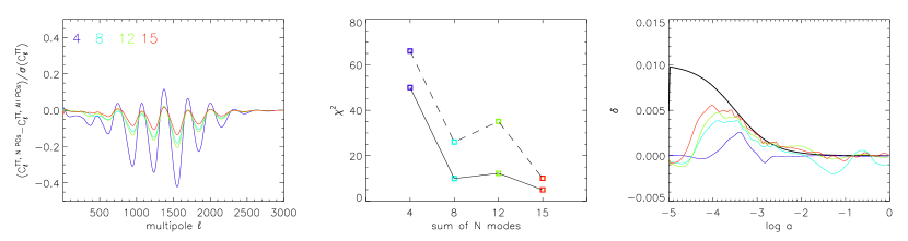
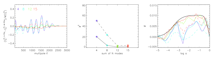
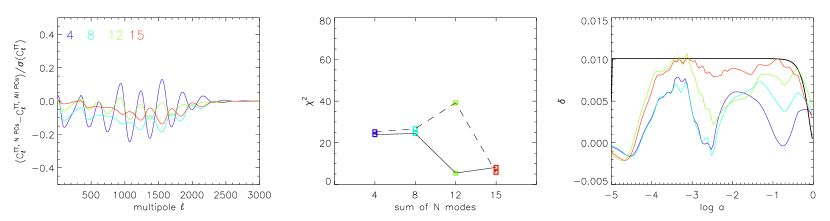
Figure 8: PCA of three models of early dark energy – dark radiation (top row), aether (middle row), and Doran-Robbers (bottom row) – is compared to the exact models in terms of the observable CMB power spectrum. The left column shows the deviation in the temperature power spectrum for the sum of the first 4, 8, 12, 15 modes using $S/N$ ordering of the modes (see Fig. 6). The $\chi^{2}$ of the deviations summing over multipoles is in the middle panels, with the dashed curve using ordering by $\sigma_{i}$ instead. Reconstruction of the theoretical $\delta(a)$ appears in the right panels; note how only certain epochs need be fit well to reproduce the observable CMB. For the aether model (middle row) dashed curves show also the $\sigma_{i}$ ordering results for the $N=8$, 15 cases, which do much worse than $S/N$ ordering.

The numbers of PCs required to ensure an accurate estimation of the observables, say $\chi^{2}<10$ (summed over 3000 multipoles), is generally greater than 10, rendering cumbersome a straight application of mode amplitudes as parameters in a Monte Carlo simulation. (And recall that for a model independent analysis we do not know a priori the $S/N$ ordering, so one would need to include many more PCs using $\sigma_{i}$ ordering.) Moreover, PCs per se are not always easy to interpret in terms of physical effects. Therefore it is both clearer and more efficient to use the PCA instead to guide an effective, low order binning basis.

V Conclusions

Our knowledge of the expansion history of our universe, even at the level of degree of matter domination or radiation domination at early epochs, is remarkably imprecise. Cosmic microwave background radiation measurements from ACT, Planck, and SPT (and later ACTpol and SPTpol) will shed light on the times around recombination and reionization. We quantify the model independent state of our knowledge through a combination of redshift bin and principal component analysis, finding that subpercent level constraints will be placed by Planck over $\log a=[-2.5,-5]$ for a bandwidth of $\Delta\log a=0.5$.

CMB data will address one of the key aspects of dark energy – its persistence, a characteristic of many high energy physics origins – and we find that several different classes of early dark energy are well separated in PCA space. The limits can also be interpreted in terms of the number of effective relativistic species, $N_{\rm eff}$, such as an extra neutrino type, with current data mildly preferring further contributions. A thermal relativistic neutrino species adds 23% to the photon energy density, so $\delta=0.13\,\Delta N_{\rm eff}$, giving tight limits on extra relativistic degrees of freedom from the forthcoming data.

We explore three specific models, representing different classes for early dark energy, possibly corresponding to different physical origins. The commonly used Doran-Robbers form has a dark energy fraction $\Omega_{e}$ that is constant through the recombination epoch. We also investigate a dark radiation model with $\Omega_{de}(a)$ rising to the past and a barotropic aether model with $\Omega_{de}(a)$ falling to the past, and find that the dominant PC mode is well able to distinguish between these behaviors. Since the amplitude of that mode is greatest for the Doran-Robbers model, we expect that data constraints on $\Omega_{e}$ in the other classes will be weaker than in this model (such as from reichardt using current CMB data), allowing for nonnegligible persistence of dark energy (see rdof for further demonstrations of this). Our general approach, however, does not rely on assuming the form for the new component or expansion deviation.

Figure 3 is in a sense the textbook picture of what Planck CMB data will say in a model independent manner about early universe expansion. For postrecombination epochs this will improve with further ground based polarization measurements (especially of CMB lensing) and inclusion of growth of structure data. Understanding early expansion is in fact crucial for accurate interpretation of large scale structure, and feeds directly into the early time gravitational growth calibration parameter $g_{\star}$ gstar ; ignorance of this can bias cosmological parameter estimation and tests of gravity.

Expansion history is not the whole story as the effective fluid behind the expansion deviations has perturbations and can have internal degrees of freedom. We treat the perturbations consistently – the dark radiation and barotropic aether models for example have sound speeds different from the speed of light. We do not include viscosity, however, as the data has poor leverage on this cold ; rdof ; smithdaszahn . Another difficulty for model independent analysis is having $\delta<0$, since perturbations are difficult to treat when the effective density deviation passes through zero; models such as nonthermal neutrinos, with energy densities below the standard, could realize such a condition. We will consider such cases in future work.

Principal component analysis provides a valuable guide to the key epochs of sensitivity and the amount of information contributed from different times. However, we emphasize and demonstrate that the raw uncertainty $\sigma_{i}$ on an eigenmode has very limited meaning; the first 15 modes ordered by $\sigma_{i}$ can give a highly inaccurate reconstruction relative to a smaller number of modes ordered by signal to noise. Redshift bins can be more clearly interpreted. Employing the best aspects of each can result in physically clear, well characterized expansion history constraints.

- (1) S.M. Carroll & M. Kaplinghat, Phys. Rev. D 65, 063507 (2002) [arXiv:astro-ph/0108002]
- (2) S. Galli, A. Melchiorri, G.F. Smoot, O. Zahn, Phys. Rev. D 80, 023508 (2009) [arXiv:0905.1808]
- (3) M. Doran and G. Robbers, JCAP 0606, 026 (2006) [arXiv:astro-ph/0601544]
- (4) E. Calabrese, D. Huterer, E.V. Linder, A. Melchiorri, L. Pagano, Phys. Rev. D 83, 123504 (2011) [arXiv:1103.4132]
- (5) E.J. Copeland, M. Sami, S. Tsujikawa, Int. J. Mod. Phys. D 15, 1753 (2006) [arXiv:hep-th/0603057]
- (6) S. Das, T.A. Marriage, P.A.R. Ade et al., ApJ 729, 62 (2011); J. Dunkley, R. Hlozek, J. Sievers et al., ApJ 739, 52 (2011)
- (7) E. Shirokoff, C.L. Reichardt, L. Shaw et al., ApJ 736, 61 (2011); R. Keisler, C.L. Reichardt, K.A. Aird et al., ApJ 743, 28 (2011)
- (8) E.V. Linder & T.L. Smith, JCAP 1106, 001 (2011) [arXiv:1009.3500]
- (9) E.V. Linder, Phys. Rev. D 82, 063514 (2010) [arXiv:1006.4632]
- (10) D. Huterer & G. Starkman, Phys. Rev. Lett. 90, 031301 (2003) [arXiv:astro-ph/0207517]
- (11) W. Hu, ApJ 506, 485 (1998) [arXiv:astro-ph/9801234]
- (12) A. Lewis, A. Challinor, & A. Lasenby, ApJ 538, 473 (2000) [arXiv:astro-ph/9911177]; http://camb.info
- (13) Planck Collaboration, P.A.R. Ade, N. Aghanim et al., A&A, 536, A1 (2011); http://planck.esa.int
- (14) W. Hu & T. Okamoto, Phys. Rev. D 69, 043004 (2004) [arXiv:astro-ph/0308049]
- (15) S. Leach, MNRAS 372, 646 (2006) [arXiv:astro-ph/0506390]
- (16) M.J. Mortonson & W. Hu, ApJ 672, 737 (2008) [arXiv:0705.1132]
- (17) R. de Putter & E.V. Linder, Astropart. Phys. 29, 424 (2008) [arXiv:0710.0373]
- (18) C. Dvorkin & W. Hu, Phys. Rev. D 82, 043513 (2010) [arXiv:1007.0215]
- (19) D.P. Finkbeiner, S. Galli, T. Lin, T.R. Slatyer, Phys. Rev. D 85, 043522 (2012) [arXiv:1109.6322]
- (20) R. de Putter & E.V. Linder, arXiv:0812.1794
- (21) E.V. Linder & R.J. Scherrer, Phys. Rev. D 80, 023008 (2009) [arXiv:0811.2797]
- (22) C.L. Reichardt, R. de Putter, O. Zahn, Z. Hou, ApJL 749, L9 (2012) [arXiv:1110.5328]
- (23) E.V. Linder, Phys. Rev. D 79, 063519 (2009) [arXiv:0901.0918]
- (24) E. Calabrese, R. de Putter, D. Huterer, E.V. Linder, A. Melchiorri, Phys. Rev. D 83, 023011 (2011) [arXiv:1010.5612]
- (25) T.L. Smith, S. Das, O. Zahn, Phys. Rev. D 85, 023001 (2012) [arXiv:1105.3246]