Truncated Lévy Flights and Weak Ergodicity Breaking in the Hamiltonian Mean Field Model

Abstract

The dynamics of the Hamiltonian mean field model is studied in the context of continuous time random walks. We show that the sojourn times in cells in the momentum space are well described by a one-sided truncated Lévy distribution. Consequently the system is non-ergodic for long observation times that diverge with the number of particles. Ergodicity is attained only after very long times both at thermodynamic equilibrium and at quasi-stationary out of equilibrium states.

Ergodicity is a fundamental concept in statistical mechanics birkhoff ; kinchin and essentially states that ensemble and time averages are equal over a single trajectory of the system or, equivalently, that the sojourn time on a given region is proportional to the ensemble measure. For particles subjected to an external potential, ergodicity implies that time averages over a single particle trajectory is equal to the average over many particles at a fixed time. The latter case has recently been observed experimentally for the diffusion of molecules on a nanostructured porous glass feil . Strong ergodicity breaking occurs if some region in the phase space is not accessible by the system trajectory. On the other hand weakly non-ergodic behavior corresponds to a situation where every state can be reached but the occupation statistics is not equal to the ensemble measure bouchaud . The statistical mechanics of a system with weak ergodicity breaking, henceforth called weakly non-ergodic, in the context of Continuous Time Random Walks (CTRW) was addressed by Rebenshtok and Barkai weba . The system can be in $M$ different states, such that a given observable ${\cal O}$ admits the respective $M$ values ${\cal O}_{k}$ for $k=1,\ldots,M$. The time average of this observable is then

$$\overline{\cal O}=\frac{1}{t_{\rm tot}}\sum_{k=1}^{M}t_{k}^{(r)}{\cal O}_{k},\hskip 14.22636ptt_{\rm tot}=\sum_{i=k}^{M}t_{k}^{(r)},$$ (1)

where $t_{k}^{(r)}$ is the residence time, i. e. the total time spent by the system in state $k$ and $t_{\rm tot}$ the total observation time. The sojourn time $t_{k}^{(j)}$ is the time spent in state $k$ during the $j$-th visitation, and therefore $t_{k}^{(r)}=\sum_{j}t_{k}^{(j)}$. Owing to Lévy generalized central limit theorem, the probability distribution of residence time $t_{k}^{(r)}$ can be described by a one-sided Lévy distribution $f^{(\alpha)}_{k}(t)$ with characteristic function weba ; Samorodnitsky :

$$\psi_{k}(z)=\exp\left\{-\gamma_{k}|z|^{\alpha}\left[1-i\tan\left(\pi\alpha/2\right){z}/{|z|}\right]\right\},$$ (2)

for $0<\alpha\leq 2$ and $\alpha\neq 1$, $\alpha=2$ corresponding to the Gaussian distribution, and $\gamma_{k}$ is a constant scale factor Samorodnitsky . An important feature is that the moments $\langle t^{\mu}\rangle$ of the Lévy distribution diverge for $\mu>\alpha$. The distribution of the possible different values of the time averages $\overline{\cal O}$ is given by weba :

$$F^{(\alpha)}(\overline{\cal O})=-\frac{1}{\pi}\lim_{\epsilon\rightarrow 0}{\rm Im}\left\{\left[\sum_{k=1}^{M}\rho_{k}(\overline{\cal O}-{\cal O}_{k}+i\epsilon)^{\alpha/2-1}\right]\left[{\sum_{k=1}^{M}\rho_{k}(\overline{\cal O}-{\cal O}_{k}+i\epsilon)^{\alpha/2}}\right]^{-1}\right\}.$$ (3)

In the limit $\alpha\rightarrow 2$ Eq. (3) reduces to $F^{(2)}(\overline{\cal O})=\delta(\overline{\cal O}-\langle{\cal O}\rangle)$, where $\langle{\cal O}\rangle=\sum_{k}\rho_{k}{\cal O}_{k}$, and the coefficients $\rho_{k}$ are stationary probabilities. As far as $\alpha\neq 2$ and consequently $F^{(\alpha)}\neq\delta(\overline{\cal O}-\langle{\cal O}\rangle)$ the system is weakly non-ergodic. The extension of this approach for cells with different occupation statistics is given in Ref. venegeroles . Examples of weakly non-ergodic systems include laser cooling of trapped atoms saubamea , diffusion of lipid granules in living cells jeon , blinking quantum dots brokmann ; margolin and glass dynamics bouchaud . In this paper we show that a classical Hamiltonian system with long-range interaction also displays a weakly non-ergodic behavior.

Systems with long-range interactions are characterized by a pair-interaction potential decaying asymptotically as $r^{-a}$, $a<D$ with $D$ the spatial dimension dauxois . These systems have drawn some attention in the last two decades physrep ; proc1 ; proc2 ; proc3 , and have unusual properties such as anomalous diffusion, aging, negative heat capacity at equilibrium, non-Gaussian quasi-stationary states and a relaxation time to equilibrium diverging with the number $N$ of particles. This last feature seems ubiquitous in such systems and is related to a very long time required to attain ergodicity, as we explicitly show bellow for one model system as a preliminary step of a thorough investigation of general classes of long-range interacting systems. Despite great interest, their dynamics is not completely understood due to inherent difficulties in both analytic and numerical approaches. A few toy models were introduced in the literature in order to simplify the understanding of their intricate behavior. Among them we mention the Hamiltonian Mean Field (HMF) model hmforig , which has become a sort of ground test for many numerical and analytic studies, and defined by the Hamiltonian:

$$H(p,\theta)=\frac{1}{2}\sum_{i=1}^{N}p_{i}^{2}+\frac{1}{2N}\sum_{i,j=1}^{N}\left[1-\cos(\theta_{i}-\theta_{j})\right].$$ (4)

This is a solvable system at equilibrium and can be interpreted as consisting of $N$ classical rotors globally coupled with unit moment of inertia hmforig ; metodo . It has a second order phase transition from a spatially homogeneous to an inhomogeneous phase, and a rich structure of non-equilibrium phase transitions noneq . In the limit $N\rightarrow\infty$ it is described by the mean field Vlasov kinetic equation braun . Thence we only have to consider the dynamics of a single particle evolving in the mean field of the remaining particles. Quasi-stationary states thus correspond to the infinite number of stable stationary states of the Vlasov equation. For finite $N$, small collisional corrections must be considered resulting in a secular evolution.

In the present letter the ergodic properties of the HMF model are studied by considering its dynamics as a CTRW by dividing the momentum space in finite width cells, with each cell being considered as one possible state of the system. We observe a very slow convergence of $\alpha$ in Eq. (3) to the Gaussian value $\alpha=2$ for the sojourn times in the cells. This is related to the very long relaxation time to thermodynamic equilibrium in long-range interacting systems. Indeed, as discussed in Ref. eplnos , the time of observation required for the system to attain ergodicity is of same order of magnitude as the relaxation time to equilibrium. This kind of sluggish convergence is also associated to a truncated power law tail in the sojourn times distribution mantegna ; nano . This implies that for shorter observation times the system can be considered as weakly non-ergodic, ergodicity being only attained asymptotically. One possible source of ergodicity breaking in long-range interacting systems, but not the only one, is a parametric resonance of particle motion with mean-field oscillations benetti .

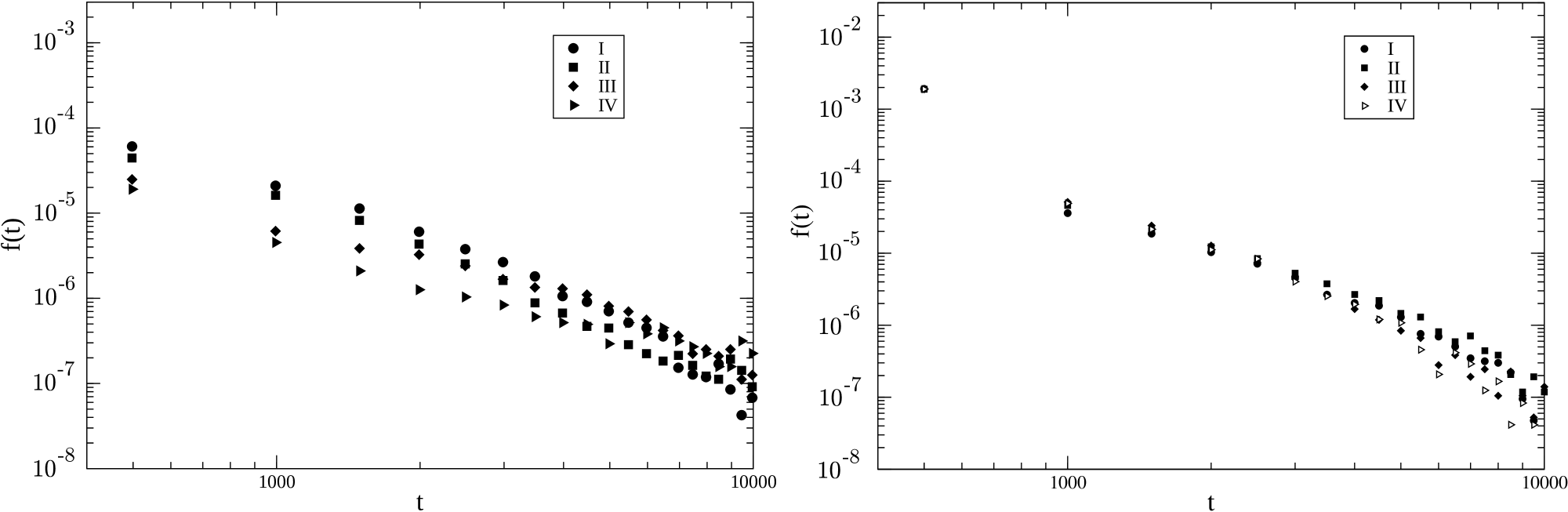
Figure 1: Left Panel: Distribution $f(t)$ of sojourn times at the thermodynamic equilibrium state for cells in momentum space in the intervals (I) $[0.0,0.4]$ (II) $[0.4,0.8]$, (III) $[0.8,1.2]$ and (IV) $[1.2,1.6]$, $N=100,000$ and total simulation time $t_{\rm tot}=10^{7}$. Right Panel: Same as left panel but for the waterbag state.

The dynamics of the HMF model is studied by performing molecular dynamics simulations for the Hamiltonian in Eq. (4). The momentum space is divided in cells of width $\Delta p$, and each cell is then taken as a different discrete state. We consider here two types of statistically stationary states, both spatially homogeneous: (i) thermodynamic equilibrium, and (ii) a stable non-Gaussian (quasi) stationary state with a waterbag one-particle constant momentum distribution in an interval $\rho(p)=1/2p_{0}$ if $-p_{0}<p<p_{0}$ and zero otherwise. Spatially homogeneous distributions imply a vanishing force in the mean-field limit, but with small fluctuations due to collisional corrections for finite $N$ causing small cumulative changes in the momentum distribution. Simulations are performed using a symplectic solver for the Hamiltonian equations implemented in a parallel code in graphic processing units eu2 . The temperature for the equilibrium case is $T=0.8$ and for the non-equilibrium case we chose $p_{0}\approx 2.68$ and total energy per particle $e=0.8$.

Figure 1 shows that the statistics of sojourn times for different cells of width $\Delta p=0.4$ are equal up to the noise level. The time evolution of the velocity of a single particle is shown in Fig. 2 illustrating clearly the trapping of the velocity in regions of the momentum space with rapid movements between different traps. This is due to the system being in a homogeneous state and therefore the interactions on each particle correspond to collisions whose effects diminish with increasing $N$, in such a way that either a rare strong collision or the cumulative effects of weaker collisions are required to extract the particle from a given cell. As the statistics of sojourn times are approximately the same for different cells, sojourn times are taken from all cells thence allowing a better statistical accuracy. Indeed, the sequence of sojourn times is obtained by considering successive time intervals between the entrance and exit of any particle in any individual cell (or state).

Figure 2: Velocity of a particle as a function of time for the Hamiltonian in Eq. (3) with $N=50,000$ and total simulation time $t_{f}=10^{6}$ for the thermodynamic equilibrium distribution.

The generalized central limit theorem lead us to expect sojourn time statistics $t^{(j)}=t_{k}^{(j)}$ for cells of width $\Delta p$ close to a one-sided Lévy distribution (with positive support). We define the empirical normalized frequency of sojourns as

$$g(t)=\frac{1}{J}\sum_{j=1}^{J}\delta\left(t-t^{(j)}\right);$$ (5)

where $t^{(j)}$ ($j=1,\ldots,J$) are the sojourn times obtained from the simulation. We drop the index $k$ associated to each cell (or state) because the sojourn time statistics are almost identical for cells with same width (see Figure 1). We may expect a truncated one sided Lévy distribution as a good approximation to describe $g(t)$. A truncated one sided Lévy distribution is defined as follows:

$$\tilde{f}^{(\alpha)}(t)=\left\{\begin{array}[]{ll}cf^{(\alpha)}(t)&0<t<L\\ 0&\mbox{otherwise}\end{array}\right.$$ (6)

where $c$ is a normalization constant, $f^{(\alpha)}(t)$ is a Lévy asymmetric distribution with characteristic function given by equation (2) and $L$ is the truncature length. In this case, as the sojourn time statistics are taken as independent of the specific cell considered, we have $\gamma_{k}=\gamma$ for all $k$.

$N$	$\alpha_{\rm eq}$	$\alpha_{\rm wb}$	$N$	$\alpha_{\rm eq}$	$\alpha_{\rm wb}$
10,000	0.67	1.00	80,000	0.57	0.66
20,000	0.62	0.82	90,000	0.57	0.65
30,000	0.60	0.74	100,000	0.57	0.64
40,000	0.59	0.70	200,000	0.55	0.61
50,000	0.58	0.69	300,000	0.55	0.61
60,000	0.58	0.67	400,000	0.55	0.62
70,000	0.57	0.66	500,000	0.56	0.63

Table 1: Values of $\alpha$ in Eq. (2) for the thermodynamic equilibrium ($\alpha_{\rm eq}$) and waterbag distribution ($\alpha_{\rm wb}$).

Truncated Lévy distributions were introduced by Mantegna and Stanley in a different context mantegna . Such functions have finite moments, and therefore the sum of random variables $X^{(n)}=\sum_{j=1}^{n}t^{(j)}$, with $t^{(j)}$ a random variable drawn from the truncated one sided Lévy distribution, converges to a Gaussian distribution. Nevertheless this convergence is extremely slow and the distribution of this sum remains close to a true stable Lévy distribution for values of $n$ that can be very large, displaying a typical scaling before a crossover to a Gaussian behavior for $n\gg n^{\star}$ where $n^{\star}$ denotes the crossover value for $n$ between the Lévy and Gaussian distributions $P(X^{(n)})$ for $X^{(n)}$. For all $n\ll n^{\star}$ the distributions $P(X^{(n)})$ collapse in the same function under the scaling:

$$\tilde{X}^{(n)}=n^{-1/\alpha}\>X^{(n)}\>\>{\rm and}\>\>P(\tilde{X}^{(n)})=n^{1/\alpha}\>P(X^{(n)}).$$ (7)

It should be pointed out that as the cells with same width are almost statistically identical, then $X^{(n)}$ can be taken as a random variable corresponding to the residence time $t^{(r)}_{k}$, and in view of that, $P\left(X^{(n)}=t\right)$ is approximately a convolution of the Lévy one sided $f^{(\alpha)}(t)$ for $t<L$.

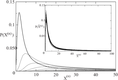
Figure 3: Density distribution $P\left(X^{(n)}=t\right)$ for the sum $X^{(n)}$ of random variables with $n=1,3,5,7,9,11$ for the equilibrium case and $N=200,000$ particles, where higher values of $n$ has a smaller maximum. The continuous line corresponds to the distribution of sojourn times ($n=1$). Inset: data collapse of the distribution functions by the scaling in Eq. (7) with $\alpha=0.55$ as the best estimate in table 1.

The shape exponent $\alpha$ in Eq. (2) for the distribution of sojourn times are given in table 1 for the equilibrium and non-equilibrium (waterbag) cases obtained using a maximum likelihood method fauerverger ; rao . The difference in the values of $\alpha$ for the equilibrium and waterbag cases with same $N$ are due to the different particle velocities and variations of the force field fluctuations around its zero average value (homogeneous state) for different energies. Figure 3 shows the sojourn times distribution function for the distributions of summed variables $X^{(n)}$ obtained by randomly summing $n$ sojourn times obtained from our simulation. The inset shows the data collapse of these distribution when rescaled according to Eq. (7) as expected for a one-sided Lévy distribution.

Figure 4: Left Panel: Histogram of the number of sojourn times for $N=50,000$ particles, $\Delta p=0.01$ and total integration time $t_{f}=10^{7}$. Right Panel: The same but with $\Delta p=0.04$. In both cases the width of each histogram bin was adjusted to be fixed in a logarithmic scale.

The existence of a truncation in the distribution of sojourn times can be made explicit by considering cells with smaller sizes, as for example $\Delta p=0.01$ and $\Delta p=0.04$. Figure 4 shows the counting histogram of sojourn times for two values of $\Delta p$. The truncation is clearly visible for $\Delta p=0.01$ while a power law tail is exhibited in the inset for $\Delta p=0.04$. Although different types of truncation are considered in the literature mantegna ; gupta , the most relevant feature for the present study is the existence of a truncation and where in the distribution it occurs.

In order to obtain an estimate of the crossover from the Lévy to Gaussian regimes we use the approach developed in reference mantegna , where the authors consider distributions of Lévy that are symmetric, although, in this problem we have one sided asymmetric distributions. Consequently, some adaptations to apply that approach must be followed.

We start defining a symmetric frequency distribution $g_{sim}(t)$ obtained from the sojourn distribution $g(t)$:

$$g_{sim}(t)=\left\{\begin{array}[]{ll}g(-t)/2&t<0;\\ &\\ g(t)/2&t>0.\end{array}\right.$$ (8)

We approximate $g_{sim}(t)$ by a symmetric truncated Lévy distribution:

$$\tilde{f}^{(\alpha)}_{sim}(t)=\left\{\begin{array}[]{ll}\displaystyle cf_{sim}^{(\alpha)}(t)&-L<t<L;\\ &\\ \displaystyle 0&\mbox{otherwise},\end{array}\right.$$ (9)

where $c$ is a constant of renormalization and $f_{sim}^{(\alpha)}(t)$ is a Symmetric Stable Lévy distribution with characteristic function given by:

$$\psi_{sim}(z)=\exp\left(-\gamma|z|^{\alpha}\right)$$ (10)

In order to show that the symmetrized sojourn time statistics for larger $\Delta p$ is well described by symmetric truncated Lévy distribution we perform a sum $X_{sim}^{(n)}$ of $n$ sojourn times randomly chosen among those obtained from our simulations but also randomly choosing its sign (this is equivalent to symmetrizing the distribution). Considering $g_{sim}(t)\approx f_{sim}^{(\alpha)}(t)$, then the probability density for small $n$ is given by mantegna :

$$P^{(n)}(0)=\frac{\Gamma(1/\alpha)}{{\pi\alpha\>(\gamma n)^{1/\alpha}}},$$ (11)

For $n$ large one has a Gaussian distribution:

$$P^{(n)}(0)=\frac{1}{\sigma\sqrt{2\pi\>n}},$$ (12)

$\sigma$ being the standard deviation of the symmetrized sojourn distribution $g_{sim}(t)$.

The crossover $n^{\star}$ from a pure Lévy to the Gaussian behavior is obtained equating equations (11) and (12); and is given by:

$$n^{\star}=A\sigma^{{2\alpha}/{(\alpha-2)}};\;\;A=\left[\sqrt{\frac{2}{\pi}}\frac{\Gamma\left(1/\alpha\right)}{\alpha\gamma^{1/\alpha}}\right]^{{2\alpha}/{(\alpha-2)}}.$$ (13)

The statistical moments of the distributions $g_{sim}(t)$ and $g(t)$ are related as follows:

$$\left<|t|^{n}\right>_{sim}=\int_{-\infty}^{\infty}|t|^{n}g_{sim}(t)dt=\int_{0}^{\infty}t^{n}g(t)dt=\left<t^{n}\right>,$$ (14)

and, also we have $\left<t^{n}\right>_{sim}=0$ for all $n$ odd. Thus, the standard deviation $\sigma=\sqrt{\left<t^{2}\right>}$ can be obtained from the second order moment of the sojourn distribution $g(t)$.

Figure 5 shows the probability $P^{(n)}(0)$ as a function of $n$. It strongly suggests that, regardless of the number of particles, the random sum process is attracted to a region close to the same symmetric stable Lévy distribution, which is well characterized by a given value of $\alpha$ and $\gamma$. We have obtained an estimate of those values by fitting the first four points of the curve corresponding to $N=400,000$. We remark that the fitted values for the shape exponent $\alpha$ are very closed to the values showed in table 1, which reinforces the consistency of the methodology based on the symmetrization of a one sided distribution. The most fundamental reason about the consistency between the two approaches is based on the fact that the asymmetric and symmetric sojourn distributions have the same power law in their tails.

Also, we clearly see from Figure 5 the crossover growth with the number of particles $N$, that is, the sum variable $X_{sim}^{(n)}$ stays longer times close to a stable Lévy distribution when the number of particles increases. This statement is confirmed by observing the right panel of Figure 6, where the value of $\sigma$ increases with the number of particles. All the remarks made above are true for both conditions used in simulations, i.e., equilibrium and waterbag.

A relation between $\left<t^{2}\right>$ and the truncature $L$ in equation (9) can be obtained (at least asymptotically for $L>>1$) through the application of a very old result obtained by the french mathematician Paul Lévy in reference levy . In this work he has showed that if the principal value of a given characteristic function, associated to a symmetric density distribution $f(t)$, is given by $-\gamma|z|^{\alpha}$, then

$$\lim_{t\rightarrow\infty}f(t)=\frac{B}{t^{1+\alpha}};\;\;B=\frac{\gamma\Gamma\left(1+\alpha\right)\sin\left(\pi\alpha/2\right)}{\pi};$$ (15)

for any $\alpha>0$ with $\sin\left(\pi\alpha/2\right)\neq 0$. This result allows us to calculate the second moment of the truncated distribution given in (9):

$$\left<t^{2}\right>_{tr}=c\int_{-L}^{L}t^{2}f_{sim}^{(\alpha)}(t)dt;\;\;c=\frac{1}{\displaystyle\int_{-L}^{L}f_{sim}^{(\alpha)}(t)dt}.$$ (16)

If $L>>1$ we have $c\approx 1$ and we get the following approximation for Eq. (16):

$$\left<t^{2}\right>_{tr}\approx 2\int_{0}^{L}t^{2}f_{sim}^{(\alpha)}dt\approx\frac{2B}{2-\alpha}L^{2-\alpha}.$$ (17)

Where the last equation in the right hand side was obtained using the result in Eq. (15). Finally, the standard deviation $\sigma^{(\alpha)}$ of the truncated Lévy (9) is given by:

$$\sigma^{(\alpha)}=\sqrt{\left<t^{2}\right>_{tr}}=\sqrt{\frac{2\gamma\Gamma(1+\alpha)\sin\left(\pi\alpha/2\right)}{(2-\alpha)\pi})}L^{(2-\alpha)/2}.$$ (18)

The calculation of the others statistical moments is straightforward and follows the same steps to obtain Eq. (18).

Equilibrium	Water-bag
$\sigma=0.64L^{0.735}$	$\sigma=0.93L^{0.690}$
$L=1.50N^{0.870}$	$L=0.14N^{0.869}$

Table 2: The relationship of $\sigma$ with the truncature $L$ and $L$ with number of particles $N$, respectively for the Equilibrium and Water-bag conditions trunc . These relations are obtained using Eq. (18) and the fitted power law in the left panel of Fig 6

Figure 6 (left panel) shows the curve of $\sigma^{(\alpha)}$ as a function of $L$ for values of the shape exponent $\alpha$ and scale factor $\gamma$ obtained by fitting in Figure 5 for both initial conditions: equilibrium and waterbag. From this figure we can conclude that for $L>50$ the Eq. (18) is already a good approximation. The divergence of the truncation $L$ can be shown by computing the second order moment $\langle t^{2}\rangle$ of the empirical sojourn times for different values of $N$ as shown in the right panel of Figure 6, where a power law increase with $N$ becomes evident. This power law combined with Eq. (18) leads to another power law linking the truncature $L$ with the number of particles $N$. In table 2 are shown the respective relations $\sigma(L)$ and $L(N)$. We remark that the truncature $L$ dependence on the number of particles $N$ seems to be given by the same power law for both conditions analyzed.

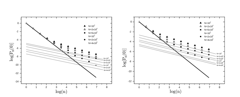
Figure 5: Left Panel: Probability density $P_{N}^{(n)}(0)$ as a function of the number $n$ of summed variables for different values of $N$ and normalized with respect to the probability for $n=1$ for the equilibrium state and averaged over 20 realizations. The continuous straight line is the curve obtained from a fitting for the initial part of the curve for $N=400,000$ with $\alpha=0.53$ and $\gamma=1.46$. Right Panel: The same as the left panel but for the waterbag state, the continuous straight line corresponds to $\alpha=0.62$ and $\gamma=2.53$. The dashed lines is the curve of $P^{(n)}(0)$ given in Eq. (12), which corresponds to the Gaussian regime. The intersection of these lines with the continuous line (the crossover) is marked with gray circles

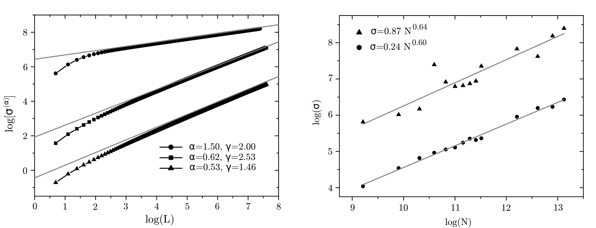
Figure 6: Left Panel: The truncated Lévy standard deviation $\sigma^{(\alpha)}$ as a function of truncature $L$ for values of $\alpha$ and $\gamma$ obtained in Fig. 5. The analogous curve for $\alpha=1.5$ and $\gamma=2.0$ is shown for comparison. The curves were translated vertically for easier viewing. The gray lines correspond to the asymptotic value given in Eq. (18). Right Panel: The empirical standard deviation of sojourn times $\sigma=\langle t^{2}\rangle$ as a function of the number $N$ of particles. Triangles correspond to the equilibrium and circles to waterbag states. The best fits for a power-law dependence of $\sigma$ on $N$ are indicated in the graphics for each case.

From our computational results we can assert that the HMF model becomes ergodic only after a very long time such that the sum of sojourn times with a truncated Lévy distribution converges very slowly to a Gaussian distribution mantegna . This sum yields the distribution of residence times and also determines the ergodic properties of the system. The time required to attain ergodicity corresponds to the crossover between Lévy and Gaussian behaviors in Figure 5. For shorter times, which are effectively still very long, the system is weakly non-ergodic and tends asymptotically to the ergodic behavior for finite $N$. Our results also show that this crossover time diverges with the number of particles in the system. The results obtained in the present work are in agreement with those presented in Ref. eplnos where it is shown that the dispersion of the time average of the momentum of a single particle is non-negligible and becomes small only after a very long time of the order of the relaxation time to equilibrium, implying that time averages are equal to ensemble averages and thus leading to $F^{(\alpha)}\rightarrow\delta(\overline{\cal O}-\langle{\cal O}\rangle)$. Up to the authors knowledge this is the first time non-ergodic behavior in a system with long-range interactions is shown to be related to Lévy flights in momentum space, however a more thorough analysis for the HMF model and other models with long-range interactions is under course and will be the subject of a future publication.

A. F., T. M. R. F. and M. A. A. would like to thank CNPq and CAPES (Brazilian government agencies) for partial financial support and Z. T. O. Jr. would like to thank FAPESB for partial financial support. A. F. and T. M. R. F. would like to thank R. Venegeroles for many useful discussions. Finally, the authors would like to acknowledge the useful comments and suggestions of the referees.

References

- (1) G. D. Birkhoff, PNAS 17, 656 (1931).
- (2) A. I. Kinchin, Mathematical Foundations of Statistical Mechanics, (Dover, New York, 1949).
- (3) F. Feil, S. Naumov, J. Michaelis, R. Valiullin, D. Enke, J. Kärger and C. Bräuchle, Angew. Chem. Int. Ed. 51, 1152 (2012).
- (4) J. P. Bouchaud, J. Phys. I France 2, 1705 (1992).
- (5) A. Rebenshtok and E. Barkai, J. Stat. Phys. 133, 565 (2008).
- (6) G. Samorodnitsky and M. S. Taqqu, Stable Non-Gaussian Random Processes (Chapman & Hall/CRC, London,2000). P. Lévy, Sur les lois stables en calcul des probabilités, C. R. Acad. Sc. 126, 1284-1286 (1923).
- (7) A. Saa and R. Venegeroles, Phys. Rev. E 82, 031110 (2010).
- (8) R. N. Mantegna and H. E. Stanley, Phys. Rev. Lett. 73, 2946 (1994).
- (9) A. Figueiredo, I. M. Gléria, R. Matsushita and S. Silva, Physica A 337, 369 (2004).
- (10) H. M. Gupta and J. R. Campanha, Physica A 268, 231 (1999).
- (11) B. Saubamea, M. Leduc and C. Cohen-Tannoudji, Phys. Rev. Lett. 83, 3796 (1999).
- (12) J.-H. Jeon, V. Tejedor, S. Burov, E. Barkai and C. Selhuber-Unkel, K. Berg-Sorensen,L. Oddershede and R. Metzler, Phys. Rev. Lett. 106, 048103 (2011).
- (13) X. Brokmann, J.-P. Hermier, G. Messin, P. Desbiolles, J.-P. Bouchaud and M. Dahan, Phys. Rev. Lett. 90, 120601 (2003).
- (14) G. Margolin and E. Barkai, Phys. Rev. Lett. 94, 080601 (2005).
- (15) A. Campa, T. Dauxois and S. Ruffo, Phys. Rep. 480,57 (2009).
- (16) Dynamics and Thermodynamics of Systems with Long-Range Interactions, T. Dauxois, S. Ruffo, E. Arimondo and M. Wilkens Eds. (Springer, Berlin, 2002).
- (17) Dynamics and Thermodynamics of Systems with Long-Range Interactions: Theory and Experiments, A. Campa, A. Giansanti, G. Morigi and F. S. Labini (Eds.), AIP Conf. Proceedings Vol. 970 (2008).
- (18) Long-Range Interacting Systems, Les Houches 2008, Session XC, T. Dauxois, S. Ruffo and L. F. Cugliandolo Eds. (Oxford Univ. Press, Oxford, 2010).
- (19) T. Dauxois, S. Ruffo, E. Arimodo and M. Wilkens, Dynamics and Thermodynamics of Systems with Long-Range Interactions: An Introduction, in proc1 .
- (20) M. Antoni and S. Ruffo, Phys. Rev. E 52, 2361 (1995).
- (21) T. M. Rocha Filho, M. A. Amato and A. Figueiredo, J. Phys. A 42, 165001 (2009).
- (22) T. M. Rocha Filho, M. A. Amato, and A. Figueiredo, Phys. Rev. E 85, 062103 (2012).
- (23) A. Figueiredo, T. M. Rocha Filho and M. A. Amato, Europhys. Lett. 83, 30011 (2008).
- (24) T. M. Rocha Filho, physics.comp-ph:1212.0261.
- (25) W. Braun and K. Hepp, Commun. Math. Phys. 56 (1977) 101.
- (26) F. P. C. Benetti, T. N. Teles, R. Pakter and Y. Levin, arXiv: 1202.1810.
- (27) A. Feuerverger and P. McDunnough, J. Am. Stat. Assoc. 76, 379-387 (1981).
- (28) C. R. Rao, Linear statistical inference and its applications, 2nd Ed. (John Wiley & Sons, New York, 2002).
- (29) P. Lévy, Sur une opération fonctionnelle généralisant la derivation d’ordre non entier, C. R. Acad. Sc. 176, 1441-1443 (1923).
- (30) The results presented in Table II show the behaviour of with adjusted by a Lévy truncated distribution. However, we should point out that the behaviour of will be discussed thoroughfully in a further communication. In this paper we are showing conclusively that the sojourn time can be interpreted in the context of Lévy truncated distributions.