Fast and robust spin manipulation in a quantum dot by electric fields

Abstract

We apply an invariant-based inverse engineering method to control by time-dependent electric fields electron spin dynamics in a quantum dot with spin-orbit coupling in a weak magnetic field. The designed electric fields provide a shortcut to adiabatic processes that flips the spin rapidly, thus avoiding decoherence effects. This approach, being robust with respect to the device-dependent noise, can open new possibilities for the spin-based quantum information processing.

Coherent spin manipulation in quantum dots (QDs) spin resonance ; control-geometric phase1 ; control-geometric phase2 ; optical-control1 ; optical-control2 ; optical-control3 ; Nowack ; Petta ; Giroday is the key element in the state-of-the-art spintronics and solid-state quantum information Hanson ; Dyakonov . Accurate spin manipulation can be achieved by several techniques. One of them is the conventional electron spin resonance induced by a magnetic field oscillating at the Zeeman transition frequency spin resonance . A more robust technique is the spin manipulation with geometric Berry phases during adiabatic motion control-geometric phase2 ; control-geometric phase1 . Nowadays, there is also a growing interest in the electric control of spin using spin-orbit (SO) coupling Rashba . It has been applied to high-fidelity spin manipulation on the $100$ ns time scale Nowack ; Petta ; Giroday . This highly efficient all-electrical method has several advantages. For example, it is easy to generate time-dependent electric fields on the nanoscale by adding local electrodes and produce spin manipulation by making them Zeeman-resonant Nowack . As a result, Rabi spin oscillations appear at a frequency much smaller than the Zeeman frequency making the flip relatively slow and prone to decoherence. We shall propose here another all-electrical technique to flip spin with high fidelity via “shortcuts to adiabaticity”, in a time that can be much shorter than any decoherence time.

Recently, several shortcuts to adiabaticity have been put forward to speed up the adiabatic passage of quantum systems, and achieve a robust and fast adiabatic-like control Rice ; Berry09 ; Chen10b ; Oliver ; bec ; Chen ; Nice ; Nice2 ; 3d ; ChenPRA ; Masuda ; Adol ; Onofrio ; transport . The transitionless or counter-diabatic control algorithms proposed by Demirplak, Rice Rice , and Berry Berry09 , are designed to add supplementary time-dependent interactions that cancel the diabatic couplings of a reference process. The system then follows exactly the adiabatic trajectory of the original unperturbed process, in principle in an arbitrarily short time. Transitionless quantum drivings have been implemented in two-level systems: spins in a magnetic field Berry09 , atoms Chen10b , and Bose-Einstein condensates in optical lattices Oliver . A different shortcut is provided by inverse engineering the transient Hamiltonian bec ; Chen using Lewis-Riesenfeld invariants LR . This method has been used for time-dependent traps bec ; Chen ; Nice ; Nice2 ; 3d , atomic transport transport , and other applications Adol ; Onofrio . Although these two methods are potentially equivalent ChenPRA , their implementations and results can be quite different. Here we choose the invariant-based inverse engineering approach, since it is better suited than the transitionless driving to be produced by the desired all-electrical means.

Model.- We consider the electric control of electron spin in a QD formed in the $x$-$y$ plane of a two-dimensional electron gas confined in the $z$-direction by the coordinate-dependent material composition, under a weak magnetic field $\mathbf{B}_{0}\parallel\mathbf{z}$, as shown in Fig. 1.

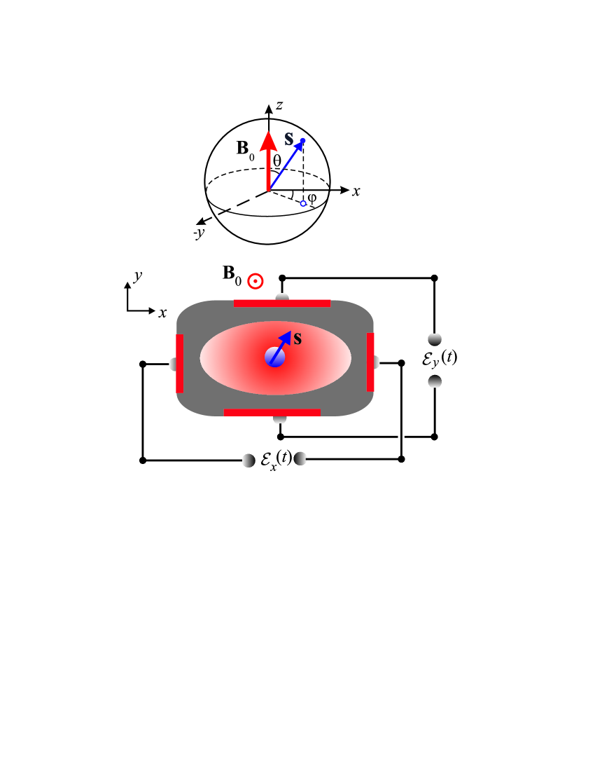
Figure 1: (Color online) Schematic diagram of spin dynamics of electron in a QD in the presence of electric fields $\mathcal{E}_{i}(t)$, and perpendicular magnetic field $\mathbf{B}_{0}\parallel{z}-$axis.

Here the total Hamiltonian $H$ of the electron interacting with the external electric field ${\bf\mathcal{E}}(t)=-\partial\textbf{A}/c\partial t$ is $H=H_{0}+H_{\rm so}+H_{\rm int},$ with Rashba

$$H_{0} = \frac{p^{2}_{x}+p^{2}_{y}}{2m}+U(x,y)+\frac{\Delta_{z}}{2}\sigma_{z},$$ (1)

$$H_{\rm so} = (-\alpha\sigma_{y}+\beta\sigma_{z})p_{x}+\alpha\sigma_{x}p_{y},$$ (2)

$$H_{\rm int} = -\frac{e}{c}\textbf{A}(t)\cdot\textbf{v},$$ (3)

where $m$ is the electron effective mass and $\sigma_{i}$ ($i=x,y,z$) are the Pauli matrices. $H_{0}$ represents the kinetic energy, the potential $U(x,y)$, and the Zeeman splitting $\Delta_{z}=g\mu_{B}B_{0}$, where $\mu_{B}$ is the Bohr magneton, and $g$ is the Landé factor. The eigenfunctions of $H_{0}$ are $\psi_{j}(x,y)\left|\sigma\right>$, where $|\sigma{\rangle}=|\pm 1{\rangle}$ is the eigenstate of $\sigma_{z}$, and the spectrum is given by $E_{j}\pm\Delta_{z}/2$, where $E_{j}$ are the orbital eigenenergies in the confinement potential.

The SO coupling is the sum of structure-related Rashba ($\alpha$) and bulk-originated Dresselhaus ($\beta$) terms for $[110]$ growth axis Golovach . The vector potential $\textbf{A}(t)$ is in the $(x,y)-$plane and corresponding spin-dependent velocity operators are

$$v_{x} = \frac{i}{\hbar}\left[H_{0}+H_{\rm so},x\right]=p_{x}/m+\beta\sigma_{z}-\alpha\sigma_{y},$$ (4)

$$v_{y} = \frac{i}{\hbar}\left[H_{0}+H_{\rm so},y\right]=p_{y}/m+\alpha\sigma_{x}.$$ (5)

We focus on the doublet $\Psi_{1}=\psi_{1}\left|1\right>$,$\Psi_{2}=\psi_{1}\left|-1\right>$, include the higher orbitals by Löwdin partition lowdin-partition ; Winkler , and reduce the full Hamiltonian into an effective $2\times 2$ one suppl material ,

$$H^{\textrm{eff}}=\frac{g\mu_{B}}{2}\left(\begin{array}[]{cc}Z&X+iY\\ X-iY&-Z\end{array}\right),$$ (8)

where $X=B_{2}(1+\xi_{y})$, $Y=(\alpha/\beta)(1+\xi_{x})B_{1}$, $Z=B_{0}+(1+\xi_{x})B_{1}$, with the effects of higher states characterized by $\xi_{x}$ and $\xi_{y}$, and the components of the designed electric field are renormalized by the factors of $1/(1+\xi_{i})$. The effective magnetic fields are expressed with the SO coupling parameters as $B_{1}=-2e\beta A_{x}/cg\mu_{B}$, and $B_{2}=-2e\alpha A_{y}/cg\mu_{B}$. The resulting electric fields are:

$$\mathcal{E}_{x}(t)=\frac{g\mu_{B}}{2e\beta}\frac{\partial B_{1}}{\partial t},~{}~{}\mathcal{E}_{y}(t)=\frac{g\mu_{B}}{2e\alpha}\frac{\partial B_{2}}{\partial t}.$$ (9)

In practice, some slowly varying electric fields can be applied to drive the state from $\Psi_{1}$ to $\Psi_{2}$ adiabatically along an instantaneous eigenstate of the Hamiltonian in Eq. (8). To accelerate the driving using the transitionless algorithm, counter-diabatic fields should be provided ChenPRA . However, the common dependence of $Y$ and $Z$ on $B_{1}$ precludes the implementation of the fast driving terms only by electric fields. In contrast, invariant-based inverse engineering naturally leads to an all-electrical driving.

Dynamical invariant and spin-flip example.- We shall design the time dependence of the external electric fields to guarantee the state transfer in some fixed time $t_{f}$ by using the dynamical $2\times 2$ invariant $I(t)$ satisfying the condition $dI(t)/dt\equiv\partial I(t)/\partial t-[H^{\textrm{eff}}(t),I(t)]/i\hbar=0$. Parametrizing the Bloch sphere (Fig. 1), by the angles $\theta$ and $\varphi$, we construct yet unknown orthogonal eigenstates $|\chi_{\pm}(t){\rangle}$ of $I(t)$ as

$$|\chi_{+}(t){\rangle}=\left(\begin{array}[]{c}\cos\displaystyle{\frac{\theta}{2}}e^{i\varphi}\\ \sin\displaystyle{\frac{\theta}{2}}\end{array}\right),|\chi_{-}(t){\rangle}=\left(\begin{array}[]{c}\sin\displaystyle{\frac{\theta}{2}}\\ -\cos\displaystyle{\frac{\theta}{2}}e^{-i\varphi}\end{array}\right).~{}$$ (14)

They satisfy $I(t)|\chi_{\pm}(t){\rangle}=\lambda_{\pm}|\chi_{\pm}(t){\rangle}$. Introducing $\lambda_{\pm}=\pm g\mu_{B}B_{c}/2$, we construct the invariant as ChenPRA

$$I(t)=\frac{g\mu_{B}}{2}B_{c}\left(\begin{array}[]{cc}\cos{\theta}&\sin{\theta}e^{i\varphi}\\ \sin{\theta}e^{-i\varphi}&-\cos{\theta}\end{array}\right),$$ (17)

where $B_{c}$ is an arbitrary constant magnetic field to keep $I(t)$ with units of energy. According to the Lewis-Riesenfeld theory, the solution of the Schrödinger equation, $i\hbar\partial_{t}\Psi=H^{\textrm{eff}}(t)\Psi$, is a superposition of orthonormal “dynamical modes”, $\Psi(t)=\sum_{n}C_{n}e^{i\alpha_{n}(t)}|\chi_{n}(t){\rangle}$ LR , where $C_{n}$ are time-independent amplitudes and $\alpha_{n}(t)$ is Lewis-Riesenfeld phase,

$$\alpha_{n}(t)=\frac{1}{\hbar}\int^{t}_{0}\langle\chi_{n}(t^{\prime})|i\hbar\frac{\partial}{\partial t^{\prime}}-H^{\textrm{eff}}(t^{\prime})|\chi_{n}(t^{\prime})\rangle dt^{\prime}.$$ (18)

From the invariant condition, $dI(t)/dt=0$, the angles $\theta$ and $\varphi$ are related to $X$, $Y$ and $Z$ by auxiliary equations

$$\dot{\theta} = \eta(X\sin\varphi-Y\cos\varphi),$$ (19)

$$\dot{\varphi} = \eta(X\cos\varphi\cot\theta+Y\sin\varphi\cot\theta-Z),$$ (20)

where $\eta=g\mu_{B}/\hbar$. Since $X$ is a function of $B_{2}$, while $Y$ and $Z$ are functions of $B_{1}$, once $\theta$ and $\varphi$ are fixed, Eqs. (19) and (20) give the effective magnetic fields

$$B_{1} = \frac{-\beta\dot{\theta}\cot\theta\cos\varphi+\beta(\dot{\varphi}+\eta B_{0})\sin\varphi}{\eta(1+\xi_{x})(\alpha\cot\theta-\beta\sin\varphi)},$$ (21)

$$B_{2} = \frac{\alpha\dot{\theta}\cot\theta\sin\varphi+\alpha(\dot{\varphi}+\eta B_{0})\cos\varphi-\beta\dot{\theta}}{\eta(1+\xi_{y})(\alpha\cot\theta-\beta\sin\varphi)},$$ (22)

from which the electric fields are calculated using Eq. (9). During the spin-flip process, there exist some time instants $t=t_{s}$ which satisfy

$$\alpha\cot\theta(t_{s})=\beta\sin\varphi(t_{s}),$$ (23)

and make the denominators of $B_{1}$ and $B_{2}$ zero. To get rid of such singularities we impose the conditions

$$\beta\sin\varphi(t_{s})\!\left[\dot{\varphi}(t_{s})+\eta B_{0}-(\beta/\alpha)\dot{\theta}(t_{s})\cos\varphi(t_{s})\right]\!=\!0,~{}~{}~{}$$ (24)

$$\alpha\cos\varphi(t_{s})\!\left[\dot{\varphi}(t_{s})+\eta B_{0}-(\beta/\alpha)\dot{\theta}(t_{s})\cos\varphi(t_{s})\right]\!=\!0,~{}~{}~{}$$ (25)

which make the numerators of $B_{1}$ and $B_{2}$ zero simultaneously. In the following example, we will show how this works.

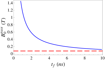
Figure 2: (Color online) Dependence of the maximum of applied magnetic field $B^{\max}_{0}$ (solid blue) on the time $t_{f}$ for a third order polynomial ansatz for $\theta$ and $\varphi$, with the parameters: $\hbar\alpha=2\times 10^{-6}$ meV$\cdot$cm, $\beta=\alpha/2$, $g=-0.44$ for GaAs. $B_{0}=0.075$ T (dashed red) corresponds to $\Delta_{z}=23$ mK.

In general, the eigenstates of the invariant are not the same as the instantaneous eigenstates of the Hamiltonian, since $I(t)$ and $H^{\rm eff}(t)$ do not commute. If we impose for $\theta$ at $t=0$ and $t_{f}$ that

$$\theta(0)=0,~{}\theta(t_{f})=\pi,~{}\dot{\theta}(0)=0,~{}\dot{\theta}(t_{f})=0,$$ (26)

then $[H^{\textrm{eff}}(0),I(0)]=0$ and $[H^{\textrm{eff}}(t_{f}),I(t_{f})]=0$, which guarantees common eigenstates at initial and final times. Moreover the state obeying Eq. (26) will flip from $|\Psi_{1}{\rangle}$ at $t=0$ to $|\Psi_{2}{\rangle}$ at $t=t_{f}$, up to phase factors, along the eigenstate $|\chi_{+}(t){\rangle}$. To design the trajectory at intermediate times we assume the polynomial ansatz $\theta=\sum_{j=0}^{3}a_{j}t^{j}$, where the $a_{j}$ can be fixed by solving the system implied by Eq. (26). This leads to $\theta(t_{f}/2)=\pi/2$, so $\cot\theta$ covers the whole $(-\infty,\infty)$ range passing through zero at $t=t_{f}/2$. This may lead to one or several times satisfying Eq. (23), as we will see below in more detail.

To determine $|\chi_{+}(t){\rangle}$ fully, we also need the trajectory for $\varphi$. As the initial and final states are the poles of the Bloch sphere, the phase $\varphi$ is not well defined there. We may nevertheless specify how the trajectory approaches them, and impose limits from the right at $t=0$, and from the left at $t=t_{f}$, for example,

$$\varphi(0^{+})=\pi/2,~{}~{}~{}~{}\varphi(t^{-}_{f})=\pi/2.$$ (27)

These conditions are not sufficient though, since we still have to deal with the singularities and their cancellation. As $\cot\theta(t_{f}/2)=0$, we may satisfy Eq. (23) and impose zeros of the denominators for $B_{1,2}$ at $t_{s}=t_{f}/2$, if $\sin\varphi(t_{f}/2)=0$. Imposing the two conditions

$$\varphi(t_{f}/2)=0,~{}~{}~{}~{}~{}~{}~{}~{}~{}~{}$$ (28)

$$\dot{\varphi}(t_{f}/2)=(\beta/\alpha)\dot{\theta}(t_{f}/2)-\eta B_{0},$$ (29)

to satisfy Eqs. (24) and (25) at $t_{s}=t_{f}/2$, we cancel the singularity there. With the conditions in Eqs. (27)-(29), we solve the third order polynomial ansatz $\varphi=\sum_{j=0}^{3}b_{j}t^{j}$ to determine $\varphi(t)$.

Explicit calculations demonstrate that for the third-order polynomial ansatz and boundary conditions imposed here, there is only one (removable) singularity at $t_{s}=t_{f}/2$ when the field $B_{0}$ is smaller than certain upper limit $B_{0}^{\max}$, shown in Fig. 2 as a function of $t_{f}$. For $B_{0}>B_{0}^{\max}$, more solutions of (23) appear [$B_{0}$ and $\sin\varphi(t)$ are coupled by Eq. (29)], which cannot be canceled with the third order polynomial. To satisfy Eqs. (24) and (25) at more than one zero of the denominators of $B_{1,2}$, one may set higher order polynomials for $\varphi$ and further conditions. This increases the bound $B_{0}^{\max}$, but also complicates the driving fields.

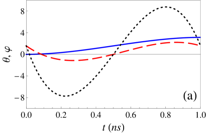
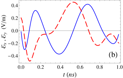
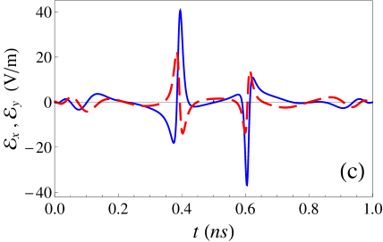
Figure 3: (Color online) For $t_{f}=1$ ns: (a) Polynomial ansatzes of auxiliary angles $\theta=\sum_{j=0}^{3}a_{j}t^{j}$ (solid blue), $\varphi=\sum_{j=0}^{3}b_{j}t^{j}$ with $B_{0}=0.15$ T (dashed red) and $B_{0}=1.05$ T (dotted black). The designed electric fields ${\mathcal{E}}_{x}$ (solid blue) and ${\mathcal{E}}_{y}$ (dashed red) by which spin flip can be realized for $B_{0}=0.15$ T (b) and $B_{0}=1.05$ T (c). Other parameters are the same as those in Fig. 2. For simplicity, we put here $\xi_{x}=\xi_{y}=0$ to skip the trivial dependence on these factors.

In the present examples, we just apply the third order polynomial ansatz with the boundary conditions in Eqs. (26)-(29), so that the applied magnetic field $B_{0}$ should not go beyond the upper limit in Fig. 2. As the upper limit field grows for smaller times $t_{f}$, this is not a problem in practice. Figure 3 shows examples of spin flip for different values of $B_{0}$.

With the functions $\theta$ and $\varphi$ fixed [see Fig. 3 (a)], the designed electric fields, $\mathcal{E}_{x}(t)$ and $\mathcal{E}_{y}(t)$, corresponding to $B_{0}=0.15$ T and $B_{0}=1.05$ T (close to the upper limit), are depicted in Fig. 3 (b) and (c). The populations (not shown) of the two spin states, given by $P_{1}=\cos^{2}{(\theta/2)}$ and $P_{-1}=\sin^{2}{(\theta/2)}$, cross each other smoothly as $\theta$ goes from $0$ to $\pi$. The choice of $B_{0}$ determines the trajectory on the Bloch sphere for a given $t_{f}$. When $B_{0}$ approaches the upper limit, the electric fields exhibit sharp peaks, see Fig. 3 (c). The smooth time-dependence in Fig. 3 (b) is well suited for the applications, while the complicated dependence in Fig. 3 (c) should be avoided. Undesirable excitation of the orbital modes does not occur here since the spin flip $t_{f}\sim 1$ ns, while the energy split of the orbital states in typical QDs exceeds $0.1$ meV. Therefore, regarding the orbital motion, our perturbation is strongly adiabatic, and no orbital excitation occurs.

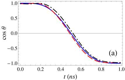
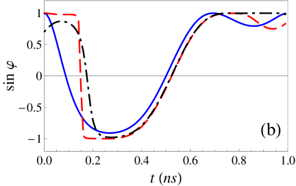
Figure 4: (Color online) Time evolution of $\cos\theta$ (a) and $\sin\varphi$ (b) for the same Hamiltonian with the designed electric fields and $B_{0}=0.15$ T, where $\epsilon=0$, $\varphi_{0}=\pi/2$ (solid blue); $\epsilon=0.01$, $\varphi_{0}=\pi/2$ (dashed red); $\epsilon=0.01$, $\varphi_{0}=\pi/4$ (dot-dashed black). Other parameters are the same as in Fig. 3.

To check the stability with respect to initialization errors, we assume now the initial state as $(\sqrt{1-\epsilon}e^{i\varphi_{0}},\sqrt{\epsilon})^{T}$ with an arbitrary phase $\varphi_{0}$ and find $\theta$ and $\varphi$ from Eqs. (19) and (20) for the same designed electric fields (Fig. 4). The final value $\theta(t_{f})$ depends on the error $\epsilon$, but insensitive to the initial phase $\varphi_{0}$, while $\varphi(t_{f})$ is sensitive to both initial conditions. Since our goal is to realize the spin flip, the final $\varphi$ is irrelevant, and the experimental effort should focus on achieving a small error $\epsilon$.

Decoherence and noise effects.- To show feasibility of our approach, we study the effects of noise and decoherence on the spin-flip fidelity. We begin with a generic approach for coupling to the incoherent environment, based on the conventional Lindblad formalism as can arise, e.g., from interaction with the conduction electron bath. The master equation reads Sipe

$$\dot{\rho}=-\frac{i}{\hbar}[H^{\textrm{eff}},\rho]-\frac{\gamma}{2}\sum_{i}[\sigma_{i},[\sigma_{i},\rho]],$$ (30)

where $\gamma$ is the dephasing rate. We introduce the Bloch vector with components $u=\rho_{1-1}+\rho_{-11}$, $v=-i(\rho_{1-1}-\rho_{-11})$, and $w=\rho_{11}-\rho_{-1-1}$, and obtain from Eq. (70)

$$\left(\begin{array}[]{ccc}\dot{u}\\ \dot{v}\\ \dot{w}\end{array}\right)=\left(\begin{array}[]{ccc}-4\gamma&\eta Z&-\eta Y\\ -\eta Z&-4\gamma&\eta X\\ \eta Y&-\eta X&-4\gamma\end{array}\right)\left(\begin{array}[]{ccc}u\\ v\\ w\end{array}\right).$$ (40)

We solve Eq.(40) numerically and calculate fidelity $F=|{\langle}-1|\Psi(t_{f}){\rangle}|$, see Fig. 5. For $\gamma t_{f}\ll 1$ the time-dependent perturbation theory 3d yields the bound $F\gtrsim 1-2\gamma t_{f}$. Since the induced flip occurs very fast, it can overcome the main danger for the low-temperature spin manipulation in QDs coming from the hyperfine coupling to the nuclear spins, where the decoherence times exceed $100$ ns Nowack .

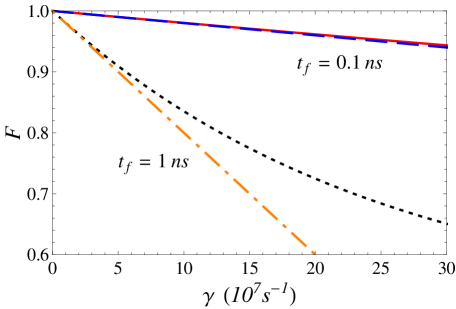
Figure 5: (Color online) Fidelity as a function of $\gamma$ for different times $t_{f}=0.1$ ns (solid red) and $t_{f}=1$ ns (dotted black). The fidelity estimated from perturbation theory is also compared, for $t_{f}=0.1$ ns (dashed blue, undistinguished) and $t_{f}=1$ ns (dot-dashed orange). $B_{0}=0.15$ T and other parameters are the same as in Fig. 2.

Another source of decoherence is the device-dependent noise in the electric field acting on the spin. This can be important when the relatively weak electric fields are applied. We analyze in detail the effect of this noise and find that our method is robust to this randomness in suppl material-2 .

Conclusions and outlook.- We have proposed a fast and robust method to flip electron spin in a QD with SO coupling and weak perpendicular magnetic field. The spin-flip process, designed by Lewis-Riesenfeld invariants, is faster than the decoherence for any known low-temperature dephasing mechanism. This method can be further complemented by optimal control theory for time- and energy-minimization subjected to different physical constraints Boscain . Implementation of this technique will allow for high-fidelity spin-manipulation for quantum information processing.

Note added: We have corrected errors in the published version.

We acknowledge funding by the Basque Government (Grants No. IT472-10 and BFI-2010-255), Ministerio de Ciencia e Innovacion (Grant No. FIS2009-12773-C02-01), UPV/EHU program (UFI 11/55), and National Natural Science Foundation of China (Grant No. 61176118) and Shanghai Rising-Star Program (Grant No. 12QH1400800).

Appendix A I. Hamiltonian reduction

Here we give the details on the derivation of the effective $2\times 2$ Hamiltonian [Eq. (6)] in the paper. For simplicity we consider a 4-level system. The total Hamiltonian is $H=H_{0}+H_{\rm so}+H_{\rm int}$. In the basis of two lowest spin-split orbital states,

$$H_{0}=\left(\begin{array}[]{cccc}E_{1}+\Delta_{z}/2&0&0&0\\ 0&E_{1}-\Delta_{z}/2&0&0\\ 0&0&E_{2}+\Delta_{z}/2&0\\ 0&0&0&E_{2}-\Delta_{z}/2\end{array}\right),$$ (45)

where $\Delta_{z}$ is the Zeeman splitting, and

$$H_{\rm so}+H_{\rm int}=\left(\begin{array}[]{cccc}-\displaystyle{\frac{e}{c}}\beta A_{x}&-\displaystyle{\frac{e}{c}}\alpha(iA_{x}+A_{y})&(\beta-\tilde{A}_{x})\overline{p}_{x}-\tilde{A}_{y}\overline{p}_{y}&\alpha(i\overline{p}_{x}+\overline{p}_{y})\\ \displaystyle{\frac{e}{c}}\alpha(iA_{x}-A_{y})&\displaystyle{\frac{e}{c}}\beta A_{x}&\alpha(-i\overline{p}_{x}+\overline{p}_{y})&-(\beta+\tilde{A}_{x})\overline{p}_{x}-\tilde{A}_{y}\overline{p}_{y}\\ (-\beta+\tilde{A}_{x})\overline{p}_{x}+\tilde{A}_{y}\overline{p}_{y}&-\alpha(i\overline{p}_{x}+\overline{p}_{y})&-\displaystyle{\frac{e}{c}}\beta A_{x}&-\displaystyle{\frac{e}{c}}\alpha(iA_{x}+A_{y})\\ \alpha(i\overline{p}_{x}-\overline{p}_{y})&(\beta+\tilde{A}_{x})\overline{p}_{x}+\tilde{A}_{y}\overline{p}_{y}&\displaystyle{\frac{e}{c}}\alpha(iA_{x}-A_{y})&\displaystyle{\frac{e}{c}}\beta A_{x}\end{array}\right),~{}~{}~{}~{}$$ (50)

with $\overline{p}_{i}={\langle}\psi_{1}|{p}_{i}|\psi_{2}{\rangle}$ and $\tilde{A}_{i}\equiv eA_{i}/mc$.

Our aim is to flip the spin between two levels taking into account the effects from orbital motion and the influence of the other levels. As the energy gap of the orbital states is much larger than the Zeeman splitting $\Delta_{z}$, the Löwdin partition lowdin-partition ; Winkler will enable us to obtain an effective $2\times 2$ matrix Hamiltonian. We split the total Hamiltonian $H$ into four blocks $\hat{Q}$, $\hat{B}$, $\hat{C}$, $\hat{C}^{\dagger}$, each of which is a $2\times 2$ matrix,

$$H=\left(\begin{array}[]{cc}\hat{Q}&\hat{C}\\ \hat{C}^{\dagger}&\hat{B}\end{array}\right).$$ (53)

The time-independent Schrödinger equation can be formally written as

$$\hat{Q}\bm{F}+\hat{C}\bm{G} = E\bm{F},$$ (54)

$$\hat{C}^{\dagger}\bm{F}+\hat{B}\bm{G} = E\bm{G},$$ (55)

Substituting the formal solution of Eq. (55), $\bm{G}=(E-\hat{B})^{-1}C^{\dagger}\bm{F}$, into Eq. (54), we get a closed equation for $\bm{F}$,

$$\hat{Q}\bm{F}+\hat{C}(E-\hat{B})^{-1}C^{\dagger}\bm{F}=E\bm{F}.$$ (56)

Therefore, the effective Hamiltonian including the effects from $\hat{B}$, $\hat{C}$ and $\hat{C}^{\dagger}$ in this subspace is given by $H^{\textrm{eff}}\rightarrow\hat{Q}+\hat{C}(E-\hat{B})^{-1}C^{\dagger}.$

Assuming that the electric field is not strong enough to excite other orbital states, namely, $e\max\left(\left|A_{x}\overline{p}_{x}\right|,\left|A_{y}\overline{p}_{y}\right|\right)/mc\ll E_{2}-E_{1}$, and keeping the first order term of the spin-orbit coupling constant, we obtain the effective Hamiltonian

$$H^{\textrm{eff}}=\left(\begin{array}[]{cc}E_{1}+h^{0}_{11}+h_{11}&h^{0}_{12}+h_{12}\\ h^{0}_{21}+h_{21}&E_{1}+h^{0}_{22}+h_{22}\end{array}\right),$$ (59)

where

$$h^{0}_{11} = -h^{0}_{22}=\Delta_{z}-\frac{e}{c}\beta A_{x},$$ (60)

$$h^{0}_{12} = h^{0*}_{21}=-\frac{e}{c}\alpha(iA_{x}+A_{y}),$$ (61)

$$h_{11} = -h_{22}=-2\frac{e\beta}{mc}\frac{\overline{p}_{x}\left(A_{x}\overline{p}_{x}+A_{y}\overline{p}_{y}\right)}{E_{2}-E_{1}},$$ (62)

$$h_{12} = h_{21}^{*}=-2\frac{e\alpha}{mc}\frac{\left(A_{x}\overline{p}_{x}+A_{y}\overline{p}_{y}\right)\left(i\overline{p}_{x}+\overline{p}_{y}\right)}{E_{2}-E_{1}}.$$ (63)

By a simple shift we may ignore the common term $E_{1}$ on the diagonal, and finally express the Hamiltonian as

$$H^{\textrm{eff}}=\frac{g\mu_{B}}{2}\left(\begin{array}[]{cc}Z&X+iY\\ X-iY&-Z\end{array}\right),$$ (66)

where $X=B_{2}(1+\xi_{y})$, $Y=(\alpha/\beta)(1+\xi_{x})B_{1}$, $Z=B_{0}+(1+\xi_{x})B_{1}$ with $B_{1}=-2e\beta A_{x}/(cg\mu_{B})$, $B_{2}=-2e\beta A_{y}/(cg\mu_{B})$. According to perturbation theory, the effects from other states can be characterized by $\xi_{x}$ and $\xi_{y}$, $\xi_{i}=2\sum_{n>1}\left|{\langle}\psi_{1}|{p}_{i}|\psi_{n}{\rangle}\right|^{2}/[m(E_{n}-E_{1})]$, summing up all contributions.

Appendix B II. Apparatus Noise Effect

Besides the decoherence resulting from the interaction between the system and the environment introduced in the main text, we consider apparatus noise, i.e. the Hamiltonian $H^{\textrm{eff}}$ [Eq. (66)] perturbed by a stochastic part $H^{\textrm{noise}}$ describing noise from the electric field source. Therefore, the Stochastic Schrödinger equation is

$$i\hbar\frac{d}{dt}\Psi(t)=(H^{\textrm{eff}}+H^{\textrm{noise}})\Psi(t).$$ (67)

Here $H^{\textrm{noise}}=\lambda H^{\prime}\zeta(t)$, and $\lambda=\lambda_{0}\sqrt{t_{f}}$, where $\zeta(t)=dW/dt$ is heuristically the time-derivative of the Brownian motion $W$ Zoller , and $\lambda_{0}$ is the strength of the noise. We have ${\langle}\zeta(t){\rangle}=0$ and ${\langle}\zeta(t)\zeta(t^{\prime}){\rangle}=\delta(t-t^{\prime})$ because the noise should have zero mean value and should be uncorrelated at different times. $H^{\prime}$ is the part of $H^{\textrm{eff}}$ contributing from the time-dependent electric field, assumed here to be parallel to the $x$-axis for the definiteness. The resulting short-time evolution of the wave function can be statistically presented using Ito approach as amplitude noise :

$$|\Psi(t+dt){\rangle}=e^{-i\left(H^{\textrm{eff}}dt+\lambda H^{\prime}dW\right)/\hbar}|\Psi(t){\rangle},$$ (68)

where $dt$ is the infinitesimal time step and $dW$ is the corresponding noise increment in the Ito calculus Zoller . The properties of such noise provide ${\langle}dW{\rangle}=0$, ${\langle}dW^{2}{\rangle}=dt$. By expanding (68) in Taylor series, and keeping the terms with first order in $dt$ and $dW$, we obtain the increment

$$|d\Psi{\rangle}=-\frac{i}{\hbar}H^{\textrm{eff}}dt|\Psi{\rangle}-\frac{\lambda^{2}}{2\hbar^{2}}H^{\prime 2}dt|\Psi{\rangle}-\frac{i\lambda}{\hbar}H^{\prime}dW|\Psi{\rangle},$$ (69)

from which time dependence of density matrix is given by amplitude noise

$$\dot{\rho}=-\frac{i}{\hbar}[H^{\textrm{eff}},\rho]-\frac{\lambda^{2}}{2\hbar^{2}}[H^{\prime},[H^{\prime},\rho]],$$ (70)

where the second term is responsible for the decrease in the process fidelity due to the apparatus noise. The master equation (70) differentiates the amplitude-noise effect from the relaxation and decoherence, described by the conventional Lindblad master equation.

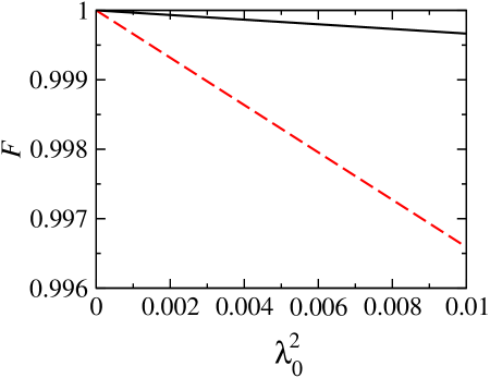
Figure 6: (Color online) Dependence of fidelity on $\lambda^{2}_{0}$, given by $t_{f}=1$ ns (solid black) and $t_{f}=0.1$ ns (dashed red). Other parameters are the same as in Fig. 2 (b) in the main text: $\hbar\alpha=2\times 10^{-6}$ meV$\cdot$cm, $\hbar\beta=10^{-6}$ meV$\cdot$cm, $g=-0.44$ for GaAs, $B_{0}=0.15$ T, $\xi_{x}=\xi_{y}=0$.

Following the same procedure to derive the Bloch equation as in the main text after Eq. (22), we obtain the corresponding equation with the source noise. By introducing three-component state vector $(u,v,w)$ we find the time evolution:

$$\left(\begin{array}[]{ccc}\dot{u}\\ \dot{v}\\ \dot{w}\end{array}\right)=\left(\begin{array}[]{ccc}-\frac{1}{2}\lambda^{2}\eta^{2}(Y^{2}+Z^{\prime 2})&\eta Z&-\eta Y\\ -\eta Z&-\frac{1}{2}\lambda^{2}\eta^{2}(X^{2}+Z^{\prime 2})&\eta X\\ \eta Y&-\eta X&-\frac{1}{2}\lambda^{2}\eta^{2}(X^{2}+Y^{2})\end{array}\right)\left(\begin{array}[]{ccc}{u}\\ {v}\\ {w}\end{array}\right),$$ (80)

where in addition to the quantities introduced in the main text, $Z^{\prime}=Z-B_{0}=(1+\xi_{x})B_{1}$. In order to analyze the effects from randomness induced by the electric field, we calculate numerically with Eq. (80) the fidelity $F=|{\langle}-1|\Psi(t_{f})|$, see Fig. 6. The high fidelity shows that our method is robust to the source noise.

References

(1) F. H. L. Koppens, C. Buizert, K. J. Tielrooij, I. T. Vink,
K. C. Nowack, T. Meunier, L. P. Kouwenhoven, and L. M. K. Vandersypen, Nature 442, 766 (2006).
(2) P. San-Jose, B. Scharfenberger, G. Schön, A. Shnirman, and G. Zarand, Phys. Rev. B 77, 045305 (2008).
(3) S. Prabhakar, J. Raynolds, A. Inomata, and R. Melnik, Phys. Rev. B, 82, 195306 (2010).
(4) A. Greilich, S. G. Carter, D. Kim, L. S. Bracker, and D. Gammon, Nat. Photon. 5, 702 (2011).
(5) T. M. Godden, J. H. Quilter, A. J. Ramsay, Y. W. Wu, P. Brereton, S. J. Boyle, I. J. Luxmoore, J. Puebla-Nunez, A. M. Fox, and M. S. Skolnick
Phys. Rev. Lett. 108, 017402 (2012).
(6) K. De Greve, Nat. Phys. 7, 872 (2011).
(7) K. C. Nowack, F. H. L. Koppens, Yu. V. Nazarov, L. M. K. Vandersypen, Science 318, 1430 (2007).
(8) J. R. Petta, H. Lu, and A. C. Gossard, Science 327, 669 (2010).
(9) A. Boyer de la Giroday, A. J. Bennett, M. A. Pooley, R. M. Stevenson, N. Sköld, R. B. Patel, I. Farrer, D. A. Ritchie, and A. J. Shields,
Phys. Rev. B 82, 241301(R) (2010).
(10) R. Hanson and D. D. Awschalom, Nature 453, 1043 (2008).
(11) M. I. Dyakonov, Spin Physics in Semiconductors, Series: Springer Series in Solid-State Sciences, Vol. 157, 2008.
(12) E. I. Rashba, Phys. Rev. B 78, 195302 (2008); E. I. Rashba and Al. L. Efros,
Phys. Rev. Lett. 91, 126405 (2003).
(13) M. Demirplak and S. A. Rice, J. Phys. Chem. A 107, 9937 (2003); J. Phys. Chem. B 109, 6838 (2005); J. Chem. Phys. 129, 154111 (2008).
(14) M. V. Berry, J. Phys. A 42, 365303 (2009).
(15) X. Chen, I. Lizuain, A. Ruschhaupt, D. Guéry-Odelin, and J. G. Muga, Phys. Rev. Lett. 105, 123003 (2010).
(16) M. G. Bason, M. Viteau, N. Malossi, P. Huillery, E. Arimondo, D. Ciampini, R. Fazio, V. Giovannetti, R. Mannella, and O. Morsch, Nat. Phys. 8, 147 (2012).
(17)J. G. Muga, X. Chen, A. Ruschhaupt, and D. Guéry-Odelin, J. Phys. B: At. Mol. Opt. Phys. 42, 241001 (2009).
(18) X. Chen, A. Ruschhaupt, S. Schmidt, A. del Campo, D. Guéry-Odelin, and J. G. Muga, Phys. Rev. Lett. 104, 063002 (2010).
(19) J. F. Schaff, X.-L. Song, P. Vignolo, and G. Labeyrie, Phys. Rev. A 82, 033430 (2010).
(20)J. F. Schaff, X. L. Song, P. Capuzzi, P. Vignolo, and G. Labeyrie, EPL 93, 23001 (2011).
(21) E. Torrontegui, X. Chen, M. Modugno, A. Ruschhaupt, D. Guéry-Odelin, and J. G. Muga, Phys. Rev. A 85, 033605 (2012).
(22) E. Torrontegui, S. Ibáñez, X. Chen, A. Ruschhaupt, D. Guéry-Odelin, and J. G. Muga, Phys. Rev. A 83, 013415 (2011).
(23) A. del Campo, Phys. Rev. A 84, 031606(R) (2011); EPL 96, 60005 (2011).
(24) S. Choi, R. Onofrio, and B. Sundaram, Phys. Rev. A 84, 051601(R) (2011).
(25) X. Chen, E. Torrontegui, and J. G. Muga, Phys. Rev. A 83, 062116 (2011).
(26) S. Masuda and K. Nakamura, Proc. R. Soc. A 466, 1135 (2010); Phys. Rev. A 84, 043434 (2011).
(27)H. R. Lewis and W. B. Riesenfeld, J. Math. Phys. 10, 1458 (1969).
(28) The term is determined by the underlying quantum well: V.N. Golovach, A.V. Khaetskii, and D. Loss, Phys. Rev. Lett. 93, 016601 (2004);
P. Stano and J. Fabian, Phys. Rev. Lett. 96, 186602 (2006).
(29) P. O. Löwdin, J. Chem. Phys. 19, 1396 (1951).
(30) R. Winkler, Spin-orbit coupling effects in two-dimensional electron and hole systems,
Springer Tracts in Modern Physics (Springer, Berlin, 2003).
(31) See Supplemental Material: I. Hamiltonian reduction.
(32) K. S. Virk and J. E. Sipe, Phys. Rev. B 72, 155312 (2005), and references therein.
(33) See Supplemental Material: II. Apparatus noise effect.
(34) U. Boscain, G. Charlot, J.-P. Gauthier, and S. Guérin, and H.-R. Jauslin, J. Math. Phys. 43, 2107 (2002).
(35) C. Gardiner and P. Zoller, Quantum Noise: A Handbook of Markovian and
Non-Markovian Quantum Stochastic Methods with Applications to Quantum Optics (Springer, Berlin, 2010)
(36) A. Ruschhaupt, X. Chen, D. Alonso, and J. G. Muga, New J. Phys. 14, 093030 (2012),
where this equation was also obtained by the Stratonovich approach.