Time-dependent barrier passage in External Noise Modulated System-reservoir Environment

Abstract

The time-dependent barrier passage of an anomalous system-reservoir coupling non-equilibrium open environment is studied where the heat bath is modulated by an external noise. The time-dependent barrier passing probability is obtained analytically by solving the generalized Langevin equation. The escaping rate and effective transmission coefficient are calculated by using of the reactive flux method in the particular case of external $\delta$-correlated noise modulated internal Ornstein-Uhlenbeck process. It is found that not all the cases of external noise modulating is harmful to the rate process. Sometimes it is even beneficial to the diffusion of the particle. There exists an optimal strength of external noise modulation for the particle to obtain a biggest probability to escape from the potential well to form a notable rate of effective net flux.

I INTRODUCTION

The diffusion model for chemical reactions has become ubiquitous in many areas of physics, chemistry and biology since its advancing by H. A. Kramers in terms of the theory of Brownian motion in phase space kramers . Several of its variants have been proposed for understanding the nature of activated processes in classical kampen ; groteh ; peterh ; epolla , semiclassical ddsray , and quantum systems clmode ; glingo ; grabet ; peteha . The majority of these treatments concern essentially with an equilibrium thermal bath at a finite temperature that simulates the reaction coordinates to cross the activation energy barrier and the inherent noise of the medium originates internally. Therefore these systems are actually classified as a thermodynamically closed system-plus-reservoir environment in contrast to the systems directly driven by external noise(s) in non-equilibrium statistical mechanics met1 . However, what will happen if the total system-reservoir environment is really open or modulated by some external forces, is the barrier crossing dynamics still amenable to the present theoretical analysis ? These problems are of valuable consideration from a microscopic point of view.

Recently, A type of system-reservoir coupling model simulating an activated rate process is studied where the heat bath is modulated by an external noise dsray2 ; dsray3 . A non-equilibrium stationary state distribution which is reminiscent of the equilibrium Boltzmann distribution in calculation of rate is proposed for this open environment by analytically solving the generalized Fokker-Planck equation and a generalized Kramers’ rate is derived via the method of flux-over-population fopm . This brings a new broad perspective for the study of anomalous activated processes in non-equilibrium open systems. However, some crucial problems such as the barrier recrossing phenomenon which is always met in an escaping process have not been concerned in these works. The time-dependent dynamical barrier escaping process in non-equilibrium open systems is far from well studied. We noticed that these can be easily achieved by the method of reactive flux rf1 ; rf2 ; jcp which is developed from the transition state theory TST1 ; TST2 ; TST3 . Therefore, following this powerful and convenient way we present in this paper a careful study on the non-equilibrium activated barrier crossing process concerning intensively on its dynamical details.

The paper is organized as follows: In Sec. II, the expression of the barrier passing probability is obtained by analytically solving the relevant generalized Langevin equation. In Sec. III, we give the time-dependent barrier escaping rate and transmission coefficient derived by using of the reaction flux method. Sec. IV serves as a summary of our conclusion where some implicate applications of this study are also discussed.

II modulated system-reservoir environment

The physical scenario depicting the modulation of the bath by an external noise lives in many different kinds of situations in forming a non-equilibrium (or non-thermal) system-reservoir coupling environment phys1 ; phys2 . For example, the simple unimolecular conversion process from $A$ to $B$ in an isomerization reaction is generally considered to be carried out in a photochemically active solvent under the influence of external fluctuating light intensity. In the reaction, fluctuations in the light intensity result in fluctuations in the polarization of the solvent molecules. Thus the effective reaction field around the reactant system gets modified. Given the required stationarity of this non-equilibrium open system is maintained, the dynamics of barrier crossing evolves amenable to the present theoretical analysis that follows.

Let us begin our study from the Hamiltonian describing a system of particles with unit mass bilinearly coupled to a harmonic reservoir that is modulated by an external noise. Mathematically it reads hami

$$H=\frac{1}{2}p^{2}+U(x)+\sum^{N}_{j=1}\left[\frac{1}{2}(p^{2}_{j}+\frac{1}{2}\omega_{j}^{2}(q_{j}-c_{j}x)^{2}\right]+H_{\textrm{int}},$$ (1)

where $\{x,p\}$ and $\{q_{j},p_{j}\}$ are the sets of coordinate and momentum variables of system and reservoir oscillators, respectively. $c_{j}x$ measures the interaction between the particle and reservoir, $U(x)$ is the potential. $H_{\textrm{int}}=\sum_{j=1}\lambda_{j}q_{j}\epsilon(t)$ represents the modulating interaction on the reservoir results from the external noise $\epsilon(t)$ which is assumed to be stationary and Gaussian with zero mean and decaying second order correlation function $\langle\epsilon(t)\epsilon(t^{\prime})\rangle_{e}=2D\psi(t-t^{\prime})$. Here $\langle\cdots\rangle_{e}$ implies the averaging over all the realizations of $\epsilon(t)$ with strength $D$ and $\psi(t)$ is a relevant memory kernel.

Eliminating the bath variables in the usual way met1 ; met2 ; met3 , a generalized Langevin equation (GLE) can be obtained as

$$\ddot{x}+\int^{t}_{0}dt^{\prime}\gamma(t-t^{\prime})\dot{x}(t^{\prime})+\partial_{x}U(x)=\zeta(t)+\varepsilon(t),$$ (2)

where $\zeta(t)=\sum_{j}c_{j}\{[q_{j}(0)-c_{j}x_{0}]\omega_{j}^{2}\textrm{cos}\omega_{j}t+p_{j}(0)\omega_{j}\textrm{sin}\omega_{j}t\}$ is the internal fluctuation force generated from the system-reservoir coupling. While $\varepsilon(t)=-\int_{0}^{t}\varphi(t-t^{\prime})\epsilon(t^{\prime})dt^{\prime}$ with $\varphi(t)=\sum_{j}c_{j}\lambda_{j}\omega_{j}\textrm{sin}\omega_{j}t$ is an additional fluctuation force resulted from the external noise $\epsilon(t)$. The anomalous form of Eq.(2) suggests that the system is under the combining government of two forcing functions. This will in no doubt lead to some novelty results.

Before reaching the central point of this article, let us firstly digress a little bit about $\zeta(t)$ and $\varepsilon(t)$. Due to its particular origin, the statistical properties of $\zeta(t)$ are determined by the initial conditions of the system-reservoir coupling environment which is assumed to be equilibrium at $t=0$ when the external noise agency has not been switched on. That is $\langle\zeta(t)\rangle=0$ and $\langle\zeta(t)\zeta(t^{\prime})\rangle=k_{B}T\gamma(t-t^{\prime})$ satisfying the fluctuation and dissipation theorem fdt1 ; fdt2 . However the statistical properties of $\varepsilon(t)$ may be enslaved to several aspects of factors such as the normal-mode density of the bath frequencies, the coupling of the system with the bath, the coupling of the bath with the external noise and the external noise itself. The very structure of $\varepsilon(t)$ suggests that this forcing function is different from a direct driving force acting on the system. Therefore after the external noise agency is switched on, the system can be regarded as being driven by an effective noise $\xi(t)$ $(=\zeta(t)+\varepsilon(t))$ whose correlation is given by

$$\langle\langle\xi(t)\xi(t^{\prime})\rangle\rangle=k_{B}T\gamma(t-t^{\prime})+2D\int^{t}_{0}dt_{1}\varphi(t-t_{1})\int^{t_{1}}_{0}dt_{2}\psi(t_{1}-t_{2})\varphi(t-t_{2}),$$ (3)

along with $\langle\langle\xi(t)\rangle\rangle=0$, where $\langle\langle\cdots\rangle\rangle$ means taking two averages independently. This relation is reminiscent of the familiar fluctuation-dissipation theorem. However, due to the appearance of the external noise intensity, it rather serves as a thermodynamic consistency condition instead.

Due to the Gaussian property of the noises $\zeta(t)$ and $\epsilon(t)$ and the linearity of the GLE, the joint probability density function $W(x,v,t;x_{0},v_{0})$ of the system oscillator must still be written in a Gaussian form adelm

$$W(x,v,t;x_{0},v_{0})=\frac{1}{2\pi|\textbf{A}(t)|^{1/2}}e^{-\frac{1}{2}\left[y^{{\dagger}}(t)\textbf{A}^{-1}(t)y(t)\right]}.$$ (4)

where $y(t)$ is the vector $[x-\langle x(t)\rangle,v-\langle v(t)\rangle]$ and $\textbf{A}(t)$ is the matrix of second moments with each component as

$$A_{11}(t) = \langle[x-\langle x(t)\rangle]^{2}\rangle,$$ (5a)

$$A_{12}(t) = A_{21}(t)=\langle[x-\langle x(t)\rangle][v-\langle v(t)\rangle]\rangle,$$ (5b)

$$A_{22}(t) = \langle[v-\langle v(t)\rangle]^{2}\rangle.$$ (5c)

The reduced distribution function can then be yielded by integrating Eq. (4) over $v$ as

$$W(x,t;x_{0},v_{0})=\frac{1}{\sqrt{2\pi A_{11}(t)}}\textrm{exp}\left[{-\frac{(x-\langle x(t)\rangle)^{2}}{2A_{11}(t)}}\right].$$ (6)

in which the average position $\langle x(t)\rangle$ can be obtained by Laplace solving the GLE. In the case of an inverse harmonic potential $U(x)=-\frac{1}{2}m\omega^{2}_{b}x^{2}$, it reads

$$\langle x(t)\rangle = \left[1+\omega^{2}_{b}\int^{t}_{0}H(t^{\prime})dt^{\prime}\right]x_{0}+H(t)v_{0}$$ (7)

where $H(t)$ namely the response function can be yielded from inverse Laplace transforming $\hat{H}(s)=[s^{2}+s\hat{\gamma}(s)-\omega^{2}_{b}]^{-1}$ with residue theorem ret1 ; ret2 .

III barrier escaping process

For the activated barrier crossing process, one of the most crucial factors that we concern is the probability of passing over the saddle point (namely also the characteristic function) which can then be determined mathematically by integrating Eq. (6) over $x$ from zero to infinity

$$\chi(x_{0},v_{0};t) = \int^{\infty}_{0}W(x,t;x_{0},v_{0})dx,$$ (8)

$$= \frac{1}{2}\textrm{erfc}\left(-\frac{\langle x(t)\rangle}{\sqrt{2A_{11}(t)}}\right),$$

which will lead to a finite real number range from 0 to 1 with 1 for reactive trajectories and 0 for nonreactive ones. The escape rate of a particle, defined in the spirit of reactive flux method by assuming the initial conditions to be at the top of the barrier, can then be yielded from

$$k(t) = \frac{1}{h}\int^{\infty}_{-\infty}dx_{0}\int^{\infty}_{-\infty}v_{0}W_{\textrm{st}}(x_{0},v_{0})\delta(x_{0}-x_{b})\chi(x_{0},v_{0};t)dv_{0}$$ (9)

in the phase space, where $W_{\textrm{st}}(x_{0},v_{{}_{0}})$ generally should be an equilibrium Boltzmann distribution that depends on the initial position and velocity of the particle. However, in the external noise modulated system-reservoir coupling environment it should be replaced by a Boltzmann form stationary probability distribution $W_{\textrm{st}}(x_{0},v_{0})=\frac{1}{Q}\textrm{exp}[-\{{\frac{v_{0}^{2}}{2D_{b}}+\frac{\tilde{U}(x_{0})}{D_{b}+\Psi(\infty)}}\}]$ which has been proved in Ref.dsray3 as a steady-state solution of the relevant Fokker-Planck equation. In the formula aforesaid, $Q$ is the partition function, $\tilde{U}(x)=U_{b}-\frac{1}{2}\Omega_{b}^{2}(x-x_{b})^{2}$ is the renormalized linear potential near the barrier top with $\Omega_{b}$ an effective frequency and $U_{b}$ the barrier height. $\Psi(\infty)$ and $D_{b}$ are two asymptotic constants to be calculated in the long time steady state (refer to Ref.dsray3 for detailed information). This stationary distribution for the non-equilibrium open system is not an equilibrium distribution but it plays the role of an equilibrium distribution of the closed system, which may, however, be recovered in the absence of the external noise.

In general, the above total rate $k(t)$ in Eq.(9) can be viewed as a generalized TST rate $k^{\textrm{TST}}=\frac{1}{Qh}e^{-U_{b}/(D_{b}+\Psi(\infty))}$ (where $[D_{b}+\Psi(\infty)]/k_{B}$ in the exponential factor defines a new effective temperature characteristic of the steady state of the non-equilibrium open system) multiplied by a factor between 0 and 1 which describes the possibility of a particle already escaped from the metastable well to recross the barrier. By substituting Eqs.(5), (7) and (8) into Eq.(9) we obtain $k(t)=\kappa(t)k^{\textrm{TST}}$ with

$$\kappa(t) = \left(1+\frac{A_{11}(t)}{D_{b}H^{2}(t)}\right)^{-1/2},$$ (10)

acting as an effective transmission factor which leads immediately to the Kramers formula for the rate constant kramers ; fopm in the absence of the external noise. As expected, both $\kappa(t)$ and $k(t)$ are the functions of the external noise strength $D$ and the coupling of noise to the bath modes. The varying of $\kappa(t)$ provides an isolated inspection on the dynamical corrections of $k(t)$ to the TST rate.

In the following calculations we rescale all the parameters so that dimensionless quantities such as $k_{B}T=1.0$ are used. We consider a particular case as an example where the external noise is $\delta$ correlated and the internal is an Ornstein-Uhlenbeck (OU) process, i.e.,

$$\langle\epsilon(t)\epsilon(t^{\prime})\rangle_{e}=2D\delta(t-t^{\prime}),$$ (11a)

$$\langle\zeta(t)\zeta(t^{\prime})\rangle=k_{B}T\frac{g^{2}}{\tau}e^{-|t-t^{\prime}|/\tau},$$ (11b)

both symmetric with respect to the time argument and assumed to be uncorrelated with each other. Where $D$ and $g$ are effective friction constants and $\tau^{-1}$ is a cutoff frequency of the system oscillator. It should be noted that for $\tau\rightarrow 0$, the internal noise shown above becomes also $\delta$-correlated. Asymptotic parameters contained in the stationary probability distribution $W_{\textrm{st}}(x_{0},v_{{}_{0}})$ are determined to be $\Omega_{b}=\omega_{b}$, $D_{b}=k_{B}T$ and $\Psi(\infty)=0$ in the particular case that we considered here.

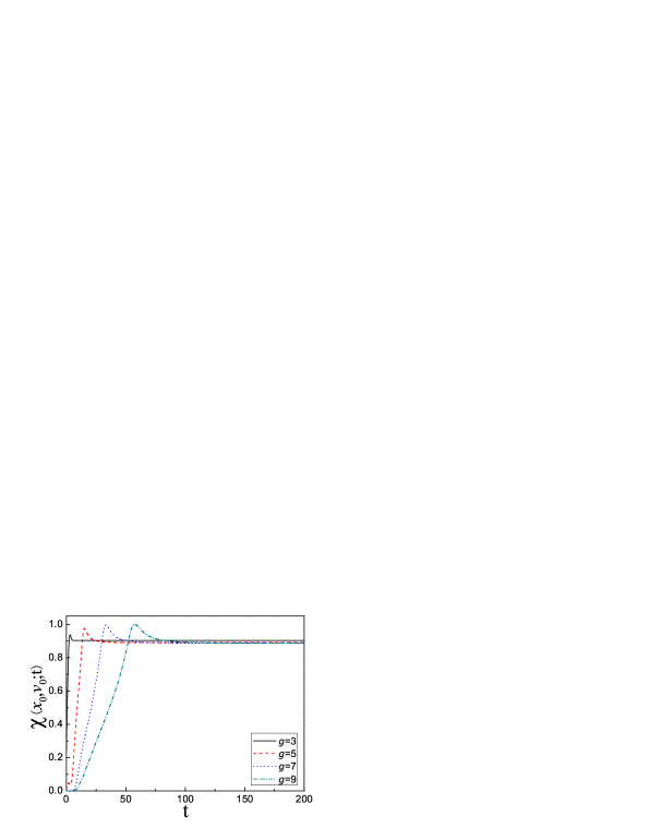
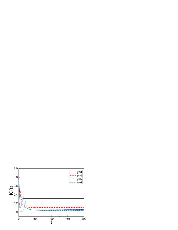
Figure 1: (Color online) Instantaneous values of $\chi(x_{0},v_{0};t)$ and $\kappa(t)$ for various strengths of purely internal noise ($D=0$). Parameters used are $\tau=3.5$, $\omega_{b}=1.2$ and $x_{0}=-1.0$, $v_{0}=0.5$ respectively.

Figure 2: Stationary values of $\chi_{\textrm{st}}$ and $\kappa_{\textrm{st}}$ as a function of the strength of internal noise $g$ where identical parameters are used as those in Fig.1.

Firstly, we present a detailed investigation on the rate process which is purely determined by the internal noise. Fig.1 gives the instantaneous values of the barrier passing probability $\chi(x_{0},v_{0};t)$ and transmission coefficient $\kappa(t)$ for various strengths of internal noise $g$ where all the system parameters are set dimensionless and particles are assumed to start from $x_{0}=-1.0$ position with initial velocity $v_{0}=0.5$. From which we can see that both $\chi(x_{0},v_{0};t)$ and $\kappa(t)$ evolve asymptotically to a stationary value in the long time limit. Meanwhile the stationary values of them decrease monotonously as the increase of the strength of internal noise. This can also be witnessed in Fig.2 where the stationary values $\chi_{\textrm{st}}$ and $\kappa_{\textrm{st}}$ are plotted as a function of the strength of internal noise $g$. This is a trivial phenomenon which can be understood in ease for a rate process. Because a hard dissipative environment is in no doubt harmful to the diffusing process. Not only will it present a frictional resistance force but also can it increase the amplitude of fluctuation. Therefore a smaller and smaller net flux is expected as the increasing of the strength of the internal noise. Particles which have already escaped from the potential well will have a big probability to recross the barrier. Correspondingly related is a small $\kappa_{\textrm{st}}$ as is shown in Fig.1.

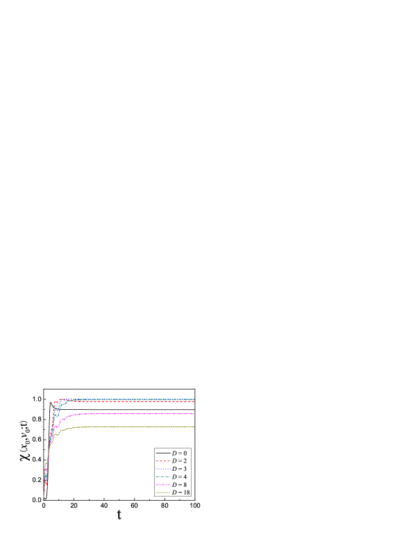
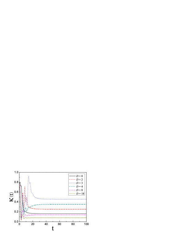
Figure 3: (Color online) Instantaneous values of $\chi(x_{0},v_{0};t)$ and $\kappa(t)$ for various strengths of external noise. Parameters used are $\tau=3.5$, $\omega_{b}=1.2$, $g=3.5$ and $x_{0}=-1.0$, $v_{0}=0.5$ for each case.

Figure 4: Stationary values of $\chi_{\textrm{st}}$ and $\kappa_{\textrm{st}}$ as a function of the strength of external noise where identical parameters are used as those in Fig.3.

In further, let us turn to the most important point of our study, i.e., what will happen if the rate process is additionally modulated by an external noise? In order to obtain a explicit elucidation of this problem we present in Fig.3 again the instantaneous values of $\chi(x_{0},v_{0};t)$ and $\kappa(t)$ at various strengths of external noise where identical system parameters are used as those in Fig.1 except for $D=0$, $2$, $3$, $4$, $8\textrm{ and }18$ respectively. The stationary values of them ($\chi_{\textrm{st}}$ and $\kappa_{\textrm{st}}$) are also exhibited as a function of the external noise strength $D$ in Fig.4 in the meantime. From which we can see a non-trivial phenomenon that both $\chi_{\textrm{st}}$ and $\kappa_{\textrm{st}}$ varies non-monotonously as the increasing of the strength of external noise. That is to say not all the cases of external noise modulating is harmful to the rate process. Sometimes it is even beneficial to the diffusing of the particle. For it can result in a bigger $\chi_{\textrm{st}}$ and $\kappa_{\textrm{st}}$ comparing to the pure internal case. This reveals, in the combining effect of internal and external noises, the particle will be able to get a biggest probability to escape from the potential well. Therefore a notable rate of net flux is expected. In further, we can infer from it that there lives an optimal strength of external noise modulation for the particle to obtain a biggest barrier escaping probability. In the particular case that is considered here this optimal value is about $D=3.4$ (dimensionless) as can be calculated following the procedures in the context foreknown.

IV SUMMARY and discussion

In summary, we have studied in this paper the time-dependent barrier passage of an external noise modulated system-reservoir coupling environment. We proposed analytically the barrier passing probability and the rate of barrier escaping. The influence of the external noise on the dynamical barrier escaping process is investigated carefully by calculating the effective transmission coefficient of an external $\delta$-correlated noise modulated internal Ornstein-Uhlenbeck process for an example. The main conclusions of our study is that not all the cases of external noise modulating is harmful to the rate process. Sometimes it is even beneficial to the diffusion of the particle. There exists an optimal strength of external noise modulation for the particle to obtain a biggest probability to escape from the potential well to form a notable rate of effective net flux.

In applications and industrial processing, the creation of a typical non-equilibrium open situation by modulating a bath with the help of an external noise is not an uncommon phenomenon. The external agency generating noise does work on the bath by stirring, pumping, agitating, etc., to which the system dissipates internally. However, provided the long-time limit of the moments for the stochastic processes pertaining to the external and internal noises characterized by arbitrary decaying correlation functions exist, the expression for the effective transmission coefficient of barrier crossing rate for the open system we derive here is fairly general. Therefore, we believe that these considerations are likely to be important in other related issues in non-equilibrium open systems and may serve as a basis for studying processes occurring within irreversibly driven environments jray ; rher and for thermal ratchet problems rdas . The externally generated non-equilibrium fluctuations can bias the Brownian motion of a particle in an anisotropic medium and may also be used for designing molecular motors and pumps.

References

- (1) H. A. Kramers, Physica (Utrecht) 7, 284 (1940).
- (2) N. G. van Kampen, Prog. Theor. Phys. 64, 389 (1978).
- (3) R. F. Grote and J. T. Hynes, J. Chem. Phys. 73, 2715 (1980).
- (4) P. Hänggi and F. Mojtabai, Phys. Rev. A 26, 1168 (1982).
- (5) E. Pollak, J. Chem. Phys. 85, 865 (1986).
- (6) P. Ghosh, A. Shit and S. Chattopadhyay, Phys. Rev. E 82, 041113 (2010).
- (7) A. O. Caldeira and A. J. Leggett, Phys. Rev. Lett. 46, 211 (1981).
- (8) H. Grabert, P. Schramm, and G. L. Ingold, Phys. Rep. 168, 115 (1988).
- (9) H. Grabert, U. Weiss, and P. Hänggi, Phys. Rev. Lett. 52, 2193 (1984).
- (10) P. Hänggi and G. L. Ingold, Chaos 15, 026105 (2005)
- (11) G. W. Ford, M. Kac and P. Mazur, J. Math. Phys. 6, 504 (1965).
- (12) S. K. Banik, J. R. Chaudhuri, and D. S. Ray, J. Chem. Phys. 112, 8330 (2000).
- (13) J. R. Chaudhuri, S. K. Banik, B. C. Chandra and D. S. Ray, Phys. Rev. E 63, 061111 (2001).
- (14) L. Farkas, Z. Phys. Chem. 125, 236 (1927).
- (15) D. J. Tannorand D. Kohen, J. Chem. Phys. 100, 4932 (1994).
- (16) D. Kohen and D. J. Tannor, J. Chem. Phys. 103, 6013 (1995).
- (17) C. Y. Wang, J. Chem. Phys. 131, 054504 (2009).
- (18) T. Seideman and W. H. Miller, J. Chem. Phys. 95, 1768 (1991).
- (19) J. M. Sancho, A. H. Romero and K. Lindenberg, J. Chem. Phys. 109, 9888 (1998).
- (20) E. Pollak and M. S. Child, J. Chem. Phys. 72, 1669 (1980).
- (21) F. Moss and P. V. E. McClintock, Noise in Nonlinear Dynamical Systems (Cambridge University, England, 1989).
- (22) W. Horsthemke and R. Lefever, Noise-Induced Transitions (Springer-Verlag, Berlin, 1984).
- (23) R. Zwanzig, J. Stat. Phys. 9, 215 (1973).
- (24) K. Lindenberg and V. Seshadri, Physica A 109, 483 (1981).
- (25) J. M. Bravo, R. M. Velasco and J. M. Sancho, J. Math. Phys. 30, 2023 (1989).
- (26) R. Kubo, Rep. Prog. Phys. 29, 255 (1966).
- (27) R. Kubo, M. Toda and N. Hashitsume, Statistical Physics II: Nonequilibrium Statistical Mechanics (Springer-Verlag, New York, 1985).
- (28) S. A. Adelman, J. Chem. Phys. 64, 124 (1976).
- (29) J. H. Mathews and R. W. Howell, Complex Analysis: for Mathematics and Engineering, 5th Ed. (Jones and Bartlett Pub. Inc. Sudbury, MA, 2006).
- (30) R. Muralidhar, D. J. Jacobs, D. Ramkrishna and H. Nakanishi, Phys. Rev. A 43, 6503 (1991).
- (31) J. R. Chaudhuri, G. Gangopadhyay and D. S. Ray, J. Chem. Phys. 109, 5565 (1998).
- (32) R. Hernandez, J. Chem. Phys. 111, 7701 (1999).
- (33) R. D. Astumian, Science 276, 917 (1997), and the references given therein.