Timeout Control in Distributed Systems Using Perturbation Analysis: Multiple Communication Links

Abstract

Timeout control is a simple mechanism used when direct feedback is either impossible, unreliable, or too costly, as is often the case in distributed systems. Its effectiveness is determined by a timeout threshold parameter and our goal is to quantify the effect of this parameter on the system behavior. In this paper, we extend previous results to the case where there are $N$ transmitting nodes making use of a common communication link bandwidth. After deriving the stochastic hybrid model for this problem, we apply Infinitesimal Perturbation Analysis to find the derivative estimates of aggregate average goodput of the system. We also derive the derivative estimate of the goodput of a transmitter with respect to its own timeout threshold which can be used for local and hence, distributed optimization.

I Introduction

Timeout control is a simple mechanism used in many systems where direct feedback is either impossible, unreliable, or too costly. This is often the case in distributed systems, where remote components cannot be observed by a controller (or several distributed controllers) and information is provided over a network with unreliable links and delays. A timeout event is scheduled using a timer which expires after some timeout threshold parameter. This defines an expected time by which some other event should occur or a “grace period” over which some response about the system state is required. If no information arrives within this period, a “timeout event” occurs and incurs certain reactions which are an integral part of the controller. In distributed systems, where usually control decisions must be made with limited information from remote components, timeouts provide a key mechanism through which a controller can infer valuable information about the unobservable system states. In fact, as pointed out in [28], timeouts are indispensable tools in building up reliable distributed systems.

This simple reactive control policy based on timeouts has been used for stabilizing systems ranging from manufacturing to communication systems [14], Dynamic Power Management (DPM) [2],[13],[22] and software systems [7],[9] among others. Despite its wide usage, quantifications of its effect on system behavior have not yet received the attention they deserve. In fact, timeout controllers are usually designed based on heuristics which may lead to poor results; an important example can be found in communication protocols, especially TCP (see [1],[14],[21],[28] and references therein). There is limited work on finding optimal timeout thresholds. For instance, in [20], a single queueing model is used for an Automatic Guided Vehicle (AGV) system and shared tester equipment. In DPM where the aim is to minimize the average power consumption, [13] and [2] propose a timeout control scheme with the aid of the theory of competitive analysis. Also, in [3], a Markov process model is used and Infinitesimal Perturbation Analysis (IPA) [4],[10] is applied to calculate the optimal timeout threshold values. In communication systems, [11],[18],[19] have attempted to find the optimal TCP retransmission timeouts by making assumptions on the probability of the transmission failure in the system. Finally, in [12] optimal web session timeouts are calculated so as to reduce the probability of falsely ending a web session in time sensitive web pages. All such approaches are limited by their reliance on the distributional information about the stochastic processes involved.

In this paper, we consider the timeout control in the context of Discrete Event Systems (DES), so that the controller output includes a response to either a timeout event or an event carrying information about network congestion. However, since stochastic DES models can be very complicated to analyze, we rely on recent advances which abstract a DES into a Stochastic Hybrid System (SHS) and, in particular, the class of Stochastic Flow Models (SFMs). A SFM treats the event rates as stochastic processes of arbitrary generality except for mild technical conditions. The emphasis in using SFMs is not in deriving approximations of performance measures of the underlying DES, but rather studying sample paths from which one can derive structural properties which are robust with respect to the abstraction made. This is the case, for instance, with many performance gradient estimates which can be obtained through IPA techniques for general SHS [6],[25]. In addition, a fundamental property of IPA in SFMs (as in DES) is that the derivative estimates obtained are independent of the probability laws of the stochastic rate processes and require minimal information from the observed sample path. This approach has proved useful in optimizing various performance metrics in serial networks [23], systems with feedback control mechanisms [27], scheduling problems [15],[16], and some multi-class models [5],[24].

In [17], we set forth a line of research aimed at quantifying how timeout threshold parameters affect the system state and ultimately its behavior and performance. We adopted a communication system model consisting of one transmitter submitting packets to a network with stochastic processing times. We showed how a SFM of a timeout-controlled distributed system can be obtained and then used to optimize the timeout threshold. This paper extends the results in [17] to multiple communication links and hence, extends this problem to broader multi-class problems with communication delays. Like [17], we directly control the timeout parameters for network communication performance. Additionally, moving from a singe class problem in [17] to multiple classes, we show how by carefully selecting the processing rate of each class, the shared communication channel operates according to a First Come First Serve (FCFS) policy. We also discuss how we can easily extend the analysis to non-FCFS frameworks. Finally, we also extend previous work on timeout control by removing any dependence on distributional information.

This paper is organized as follows: In Section II, we define the SFM of the system. In Section III, we apply IPA techniques to average goodput at each transmitter, as well as total goodput of the system aggregating the rates for all the transmitting nodes. We conclude with Section IV.

II Stochastic Flow Model (SFM)

We are interested in systems where $N$ transmitting nodes send data to their destinations through a shared channel. Associated with each node $n=1\ldots,N$, is a “class” $n$ of data packets or tasks which are to be processed in the channel and reach their destinations in a timely manner. Like the case of a single communication link, after each transmission by node $n$, a timely acknowledgement (ACK) is expected from the receiving end. For transmitter node $n$ to operate normally, the Round-Trip Transportation (RTT) time calculated for each node $n$ should be less than a timeout threshold parameter $\theta_{n}\geq 0$. If no ACK is received within $\theta_{n}$ units of time from the transmission, a timeout occurs causing node $n$ to retransmit the timed out data (previously sent at $t-\theta_{n}$) to the same destination. The control parameter vector is defined as $\boldsymbol{\theta}=[\theta_{1},\theta_{2},\ldots,\theta_{N}]^{\textsf{T}}$.

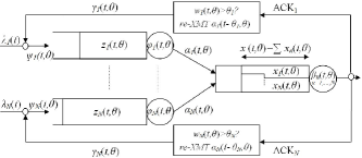
Figure 1: The SFM for the timeout system

We consider a SFM for this problem where $N$ upstream nodes are competing to get their content through a shared network channel. The channel latency represents the RTT delay in the underlying DES. The SFM for this system is shown in Fig. 1 and is observed over a finite period of time $[0,T]$. Associated with this system are several nonnegative stochastic processes all defined on a common probability space $(\Omega,\mathcal{F},P)$. The transmitters are shown as upstream nodes receiving exogenous inflow processes $\{\lambda_{n}(t)\}$, $n=1,\ldots,N$ and copy/timeout flow processes $\{\gamma_{n}(t,\boldsymbol{\theta})\}$ intended for retransmission. The process $\{z_{n}(t,\boldsymbol{\theta})\}$ models the amount of pending data to be transmitted by node $n$ and evolves according to

$$\dot{z}_{n}(t,\boldsymbol{\theta})=\frac{dz_{n}(t,\boldsymbol{\theta})}{dt^{+}}=$$

$$\left\{\begin{array}[]{ll}0&{\rm\ if\ }z_{n}(t,\boldsymbol{\theta})=0,\psi_{n}(t,\boldsymbol{\theta})\leq\phi_{n}(t,\boldsymbol{\theta})\\ \psi_{n}(t,\boldsymbol{\theta})-\phi_{n}(t,\boldsymbol{\theta})&{\rm\ otherwise}.\end{array}\right.$$ (3)

where

$$\psi_{n}(t,\boldsymbol{\theta})=\lambda_{n}(t)+\gamma_{n}(t,\boldsymbol{\theta})$$ (4)

and $\{\phi_{n}(t,\boldsymbol{\theta})\}$ is the maximal transmission rate process at node $n$. Thus, the actual transmission rate from node $n$ to the network buffer is defined as

$$\alpha_{n}(t,\boldsymbol{\theta}) =\left\{\begin{array}[]{ll}\psi_{n}(t,\boldsymbol{\theta})&{\rm\ if\ }z_{n}(t,\boldsymbol{\theta})=0,\psi_{n}(t,\boldsymbol{\theta})\leq\phi_{n}(t,\boldsymbol{\theta})\\ \phi_{n}(t,\boldsymbol{\theta})&{\rm\ otherwise}\end{array}\right.$$ (7)

In this paper, we assume that the transmitters have an infinite supply property as follows:

Assumption 1. $z_{n}(t,\theta)>0$ for all $t\in[0,T]$.

By (7), this implies $\alpha_{n}(t,\boldsymbol{\theta})=\phi_{n}(t,\boldsymbol{\theta})>0$ for all $t\in[0,T]$ , so $\phi_{n}(t,\theta)$ can henceforth be replaced by $\alpha_{n}(t,\theta)$ for the rest of the discussion.

We model the shared network channel with a buffer where the transmitted fluid from node $n$ accumulates and takes a share $x_{n}(t,\boldsymbol{\theta})\geq 0$ of the total buffer content $x(t,\boldsymbol{\theta})=\sum_{n}x_{n}(t,\boldsymbol{\theta})$. The processing rate of the fluid is governed by nonnegative service processes $\{\beta_{n}(t,\boldsymbol{\theta})\}$, $n=1,\ldots,N.$

Furthermore, for each $n$, we define the independent process $\{B_{n}(t)\}$ as the maximal processing rate of class $n$ when no other class is being processed by the network resource. Since, $\beta_{n}(t,\boldsymbol{\theta})$ is the processing rate in the presence of other fluid classes competing for a share of processing power in the network, we naturally have $\beta_{n}(t,\boldsymbol{\theta})\leq B_{n}(t)$.

At any time $t\in[0,T]$, $x_{n}(t,\boldsymbol{\theta})$ in the network follows the dynamics

$$\dot{x}_{n}(t,\boldsymbol{\theta})=\frac{dx_{n}(t,\boldsymbol{\theta})}{dt^{+}}=$$

$$\left\{\begin{array}[]{ll}0&{\rm\ if\ }x(t,\boldsymbol{\theta})=0,\alpha(t,\boldsymbol{\theta})\leq\beta(t,\boldsymbol{\theta})\\ \alpha_{n}(t,\boldsymbol{\theta})-\beta_{n}(t,\boldsymbol{\theta})&{\rm\ otherwise}\end{array}\right.$$ (10)

where $\alpha(t,\boldsymbol{\theta})=\sum_{n}\alpha_{n}(t,\boldsymbol{\theta})$ and $\beta(t,\boldsymbol{\theta})=\sum_{n}\beta_{n}(t,\boldsymbol{\theta})$. We also define the process

$$w_{n}(t,\boldsymbol{\theta})=\min_{w\geq 0}\left\{\int_{t-w}^{t}\beta_{n}(\tau,\boldsymbol{\theta})d\tau=x_{n}(t-w,\boldsymbol{\theta})\right\},$$ (11)

as the waiting time process of class $n\in\{1,\ldots,N\}$. We assume that the value of the processes $\beta_{n}(t,\boldsymbol{\theta})$ and $x_{n}(t-w,\boldsymbol{\theta})$ are known over $t\in[-w,0]$ as the initial pieces of information required to calculate $w(t,\boldsymbol{\theta})$ at $t=0$. Definition (11) has a very close relation to the “time-to-empty” process as defined in [26],[8] since one way to interpret (11) is as the earliest time it takes the server to process the content at $t-w$.

Using the waiting time process, we can define the timed-out (hence, worthless) portion of class-$n$ fluid in the network buffer for which $w_{n}(t,\boldsymbol{\theta})>\theta_{n}$. This portion needs to be retransmitted by the upstream node $n$. Under normal conditions, the network generates an acknowledgement flow indicating a successful transmission previously made at $t-w_{n}(t,\boldsymbol{\theta})$. In case of a timeout at node $n$ - i.e. the moment $w_{n}(t,\boldsymbol{\theta})$ exceeds $\theta_{n}$ - a copy of the fluid sent at time $t-\theta_{n}$ is generated and will be put back in node $n$ for retransmission. This is shown as the feedback flow process $\gamma_{n}(t,\boldsymbol{\theta})\geq 0$ in Fig. 1. To summarize, for all $t\in[0,T]$, we have

$$\gamma_{n}(t,\boldsymbol{\theta})=\left\{\begin{array}[]{ll}0&{\rm\ if\ }w_{n}(t,\boldsymbol{\theta})\leq\theta_{n}\\ \alpha_{n}(t-\theta_{n},\boldsymbol{\theta})&{\rm\ otherwise}\end{array}\right.$$ (12)

The upstream node treats this copy flow with higher priority and tries to retransmit it as soon as possible. This is inline with many retransmission-based communication protocols. Looking at Fig.1, we should explicitly show the flow $\gamma_{n}(t,\boldsymbol{\theta})$ creating contents ahead of those created by $\lambda_{n}(t)$. However, we refrained from this to avoid complicating the illustration.

We look at average goodput as the communication performance metric defined as

$$J(\boldsymbol{\theta},T) =\mathrm{E}[G(\boldsymbol{\theta},T)]$$ (13)

$$G(\boldsymbol{\theta},T) =\sum_{n}\int_{0}^{T}\bigg{[}\alpha_{n}(t,\boldsymbol{\theta})-2\gamma_{n}(t,\boldsymbol{\theta})\bigg{]}dt$$ (14)

where, like the one-dimensional problem [17], we use $2\gamma_{n}(t,\boldsymbol{\theta})$ to not only penalize the retransmissions but also to account for the worthless timed out fluid in the network buffer which should be processed by the network resource anyway.

Before proceeding, we make the following assumption on the system which we also made in [17]:

Assumption 2. The network buffer is lossless.

This assumption is merely for simplifying the exposition and can be removed at the expense of having new state variables tracking the loss volume of each class.

II-A FCFS Implementation

The definition of the waiting time (11) is contingent upon having a FCFS policy implemented in the network buffer. One of the differences between a single transmitter model in [17] is in how to ensure this policy is preserved. We achieve this by carefully selecting the network processes.

In general, depending on the processes $\beta_{n}(t,\boldsymbol{\theta})$, if two fluid particles of class $n$ and $m$, $n\neq m$ are transmitted at times $\tau_{1}$ and $\tau_{2}$, $\tau_{2}>\tau_{1}$, if $\beta_{m}(t,\boldsymbol{\theta})$ is sufficiently larger than $\beta_{n}(t,\boldsymbol{\theta})$, their order of leaving the network may be reversed. We can implement both FCFS and non-FCFS policies by carefully defining the processing rates $\beta_{n}(t,\boldsymbol{\theta})$, $n=1,\ldots,N.$ We limit the details on the non-FCFS policies to Remark 21 where it is shown that the extension of the results to the non-FCFS policies is straightforward.

Recall that $\beta_{n}(t,\boldsymbol{\theta})\leq B_{n}(t)$ since some part of the resource is consumed by other classes. Moreover, just as in the DES where a slow service for one type of customer increases the waiting time of the other customers behind it, if $B_{n}(t)$ is small, it not only means slow processing for class $n$, but also a decreasing effect on other processing rates $\beta_{m}(t,\boldsymbol{\theta})$, $m\neq n$. The availability rate of fluid class $n$ at the network server can be defined as

$$\tilde{\alpha}_{n}(t,\boldsymbol{\theta})=\alpha_{n}(t-w_{n}(t,\boldsymbol{\theta}),\boldsymbol{\theta})\quad\forall t\in[0,T].$$ (15)

Accordingly, at any time $t\in[0,T]$, the utilization of the service associated with class $n=1,\ldots,N$ is as follows:

$$\rho_{n}(t,\boldsymbol{\theta})=\frac{\tilde{\alpha}_{n}(t,\boldsymbol{\theta})}{B_{n}(t)}.$$ (16)

Hence, at each time $t$, $\rho_{n}(t,\boldsymbol{\theta})$ is a measure of how engaged the server is with the fluid of class $n$. The following theorem ensures all these characteristics are delivered by carefully defining $\beta_{n}(t,\boldsymbol{\theta}),\ n=1,\ldots,N$. Compared to [26],[8], it allows for different maximal service processes for each class.

Theorem 1. Let $w\in\mathbb{R}^{+}$. Assuming the initial conditions $w_{n}(0,\boldsymbol{\theta})\equiv w$ for all $n$, if

$$\beta_{n}(t,\boldsymbol{\theta})=\frac{\tilde{\alpha}_{n}(t,\boldsymbol{\theta})}{\sum_{m}\rho_{m}(t,\boldsymbol{\theta})}=\frac{\tilde{\alpha}_{n}(t,\boldsymbol{\theta})}{\sum_{m}\frac{\tilde{\alpha}_{m}(t,\boldsymbol{\theta})}{B_{m}(t)}},\quad\forall t\in[0,T],$$ (17)

the following statements are true:

• There exists a common waiting time process $w(t,\boldsymbol{\theta})$ such that $w_{n}(t,\boldsymbol{\theta})=w(t,\boldsymbol{\theta})$ for all $n$ and all $t\in[0,T]$.

• If $0\leq t_{1}<t_{2}$, then $t_{1}-w(t_{1},\boldsymbol{\theta})<t_{2}-w(t_{2},\boldsymbol{\theta})$

Proof: When $x(t,\boldsymbol{\theta})=0$, the buffer clearly operates according to FCFS, so we only consider the case where $x(t,\boldsymbol{\theta})>0$. By proving statement $(i)$, we show the fluid particles at the head of the queue must have arrived at the same time; Statement $(ii)$ shows that regardless of the class, fluid particles leave the system with the order they have been transmitted.
We start by proving statement $(i)$. Differentiating the term in brackets in (11) with respect to $t$ reveals

$$\beta_{n}(t,\boldsymbol{\theta})-[1-\dot{w}_{n}(t,\boldsymbol{\theta})]\beta_{n}(t-w_{n}(t,\boldsymbol{\theta}),\boldsymbol{\theta})=$$

$$[1-\dot{w}_{n}(t,\boldsymbol{\theta})]\dot{x}_{n}(t-w_{n}(t,\boldsymbol{\theta}),\boldsymbol{\theta})$$

which after regrouping the terms yields

$$\dot{w}_{n}(t,\boldsymbol{\theta})=1-\frac{\beta_{n}(t,\boldsymbol{\theta})}{\alpha_{n}(t-w_{n}(t,\boldsymbol{\theta}),\boldsymbol{\theta})}=1-\frac{\beta_{n}(t,\boldsymbol{\theta})}{\tilde{\alpha}_{n}(t,\boldsymbol{\theta})}.$$ (18)

Using (17) in the last equation gives

$$\dot{w}_{n}(t,\boldsymbol{\theta})=1-\frac{1}{\sum_{m}\rho_{m}(t,\boldsymbol{\theta})},\quad\forall t\in[0,T).$$ (19)

for which we consider the constraint $w_{n}(t)\geq 0$. Notice that the RHS is independent of $n$. Hence, with the initial condition that $w_{n}(0,\boldsymbol{\theta})\equiv w$ for all $n$, $w_{n}(t,\boldsymbol{\theta})=w_{m}(t,\boldsymbol{\theta})$ for any pair $n,m,\ n\neq m$ and the FCFS operation when $w_{n}(t,\boldsymbol{\theta})$ is defined for all $n$. Finally, we can define the waiting time dynamics of a fluid differential at the head of the network buffer as

$$\dot{w}(t,\boldsymbol{\theta})=\left\{\begin{array}[]{ll}0&{\rm\ if\ }x(t,\boldsymbol{\theta})=0\\ 1-\frac{1}{\sum_{m}\rho_{m}(t,\boldsymbol{\theta})}&{\rm\ otherwise}\end{array}\right.$$ (20)

This proves part $(i)$ in the theorem statement.

For part $(ii)$ notice that by definition, a fluid particle which is at the head of the queue at time $t$ has arrived at $t-w(t,\boldsymbol{\theta})$. Therefore, we only need to show that for any $t_{1},t_{2}\in[0,T]$ such that $t_{1}<t_{2}$, we have $t_{1}-w_{1}(t_{1},\boldsymbol{\theta})<t_{2}-w_{2}(t_{2},\boldsymbol{\theta})$. We can write $t_{1}-w(t_{1},\boldsymbol{\theta})<t_{2}-w(t_{2},\boldsymbol{\theta})$. It follows that

$$t_{1}-t_{2}<w(t_{1},\boldsymbol{\theta})-w(t_{2},\boldsymbol{\theta})$$

$$\qquad=w(t_{1},\boldsymbol{\theta})-\left[w(t_{1},\boldsymbol{\theta})+\int_{t_{1}}^{t_{2}}\dot{w}(\tau,\boldsymbol{\theta})d\tau\right]$$

$$\qquad=-\int_{t_{1}}^{t_{2}}\dot{w}(\tau,\boldsymbol{\theta})d\tau$$

$$\qquad=t_{1}-t_{2}-\int_{t_{1}}^{t_{2}}-\frac{1}{\sum_{m}\rho_{m}(\tau,\boldsymbol{\theta})}d\tau$$

which, by (20), gives

$$0<\int_{t_{1}}^{t_{2}}\frac{1}{\sum_{m}\rho_{m}(\tau,\boldsymbol{\theta})}d\tau.$$

Notice that $\frac{1}{\sum_{m}\rho_{m}(\tau,\boldsymbol{\theta})}>0$. This proves part $(ii)$ and the theorem.  With a more complicated proof, we can show the theorem statements are true even if Assumption 1 does not apply. However, we do not consider it in this paper.

Remark 1: We can come up with schemes other than FCFS and generalize the SFM analysis. For example, if by defining

$$\beta_{n}(t,\boldsymbol{\theta})=B_{n}(t)\frac{\tilde{\alpha}_{n}(t,\boldsymbol{\theta})}{\sum_{m}\tilde{\alpha}_{m}(t,\boldsymbol{\theta})},\quad\forall n.$$

we share the resource capacity according to relative availability of the fluid classes at the server, (18) becomes

$$\dot{w}_{n}(t)=1-\frac{B_{n}(t)}{\sum_{m}\tilde{\alpha}_{m}(t,\boldsymbol{\theta})},\quad\forall t\in[0,T].$$ (21)

Now, the right-hand side of this equation is $n$-dependent, which breaks the FCFS rule.

For the rest of this paper, we make the following assumption:

Assumption 3. $B_{n}(t)=B(t)$ for all $t\in[0,T]$ and $n=1,\ldots,N.$

We can remove this assumption at the expense of more complexity which diverts the focus from the main purpose of this analysis. Assumption II-A is not limiting in the present problem as the communication channels treat the packets from different sources or classes equally. Moreover, a byproduct of Assumption II-A is that

$$\beta(t,\boldsymbol{\theta}) =\sum_{n}\beta_{n}(t,\boldsymbol{\theta})=\sum_{n}\frac{\tilde{\alpha}_{n}(t,\boldsymbol{\theta})}{\sum_{m}\frac{\tilde{\alpha}_{m}(t,\boldsymbol{\theta})}{B_{m}(t)}}$$

$$=B(t)\sum_{n}\frac{\tilde{\alpha}_{n}(t,\boldsymbol{\theta})}{\sum_{m}\tilde{\alpha}_{m}(t,\boldsymbol{\theta})}=B(t),\quad\forall t\in[0,T],$$ (22)

which means the total processing rate of the channel is independent of the timeout rates chosen.

II-B Transmission Control

We say node $n$ is operating in a normal period when $w(t,\boldsymbol{\theta})\leq\theta_{n}$. In this mode, we assume that the inflow rates are determined according to the policy $\pi_{1,n}$ which is designed to increase the transmission rate $\alpha_{n}(t,\boldsymbol{\theta})$. We adopt a second policy $\pi_{2,n}$ which applies when the node is in the timeout period, i.e., $w(t,\boldsymbol{\theta})>\theta_{n}$. Policy $\pi_{2,n}$ is reactive and aims at reducing the transmission rate until the network channel comes out of the congestion and can satisfies the requirement $w(t,\boldsymbol{\theta})\leq\theta_{n}$ again. There can be many choices for the policies $\pi_{1,n}$ and $\pi_{2,n}$. For the sake of analysis, we choose the policies as follows:

$$\dot{\alpha}_{n}(t,\boldsymbol{\theta}) =f_{\alpha_{n}}(t,\boldsymbol{\theta})=\left\{\begin{array}[]{ll}r_{a}&{\rm\ if\ }w(t,\boldsymbol{\theta})\leq\theta_{n}\\ 0&{\rm\ otherwise}\end{array}\right.,$$ (25)

$$\alpha_{n}(t,\boldsymbol{\theta}) \equiv\alpha_{n,\min}{\rm\ if\ }w(t,\boldsymbol{\theta})>\theta_{n}.$$

II-C Stochastic Hybrid Model

Viewed as a SHS, we can conceive of the following SFM operation modes throughout the sample path: We refer to a period over which $x(t,\boldsymbol{\theta})>0$ and $x(t,\boldsymbol{\theta})=0$, as a Non-Empty Period (NEP) and Empty Period (EP), respectively. Moreover, we denote the periods over which $w(t,\boldsymbol{\theta})>\theta_{n}$ and $w(t,\boldsymbol{\theta})\leq\theta_{n}$ by TOP_n and NP_n, respectively.

Let $\tau_{k}$, $k=1,\ldots,K$, be the SFM event times observed in a sample path of the system over the interval $[0,T]$. We also define $\tau_{0}=0$ and $\tau_{K+1}=T$ for notational convenience and let $e_{k}$ be the event occurring at $\tau_{k}$. We are interested in the following set of events:

$$\mathcal{E}=\big{\{}E_{\lambda},E_{B},[x>0],[x= 0],[w>\theta_{n}],[w\leq\theta_{n}],$$

$$[{\tilde{\alpha}_{n}^{+}\neq\tilde{\alpha}_{n}^{-}}],[\gamma_{n}^{+}\neq\gamma_{n}^{-}]\big{\}}.$$ (26)

Here, $E_{\lambda}$ and $E_{B}$ respectively refer to random jump events in any $\lambda_{n}(t)$, $n=1,\ldots,N$ and $B(t)$ which are not affected by $\boldsymbol{\theta}$. We call the events with this property exogenous. The start and end of a NEP is marked by the events $[x>0]$ and $[x=0]$, respectively. $[w>\theta_{n}]$ and $[w\leq\theta_{n}]$ are the events defining the start and end of a TOP_n. Since these events are dependent on the system states, we categorize them as endogenous events. When a timeout $[w>\theta_{n}]$ event occurs, according to (25), $\alpha_{n}(t,\boldsymbol{\theta})$ drops. This discontinuity will then be reflected in $\tilde{\alpha}_{n}(t,\boldsymbol{\theta})$ and consequently, by (17), in $\beta_{n}(t,\boldsymbol{\theta})$. We refer to the event of $\tilde{\alpha}_{n}(t^{+},\boldsymbol{\theta})\neq\tilde{\alpha}_{n}(t^{-},\boldsymbol{\theta})$ by $[{\tilde{\alpha}_{n}^{+}\neq\tilde{\alpha}_{n}^{-}}]$. As the last system event, $[\gamma_{n}^{+}\neq\gamma_{n}^{-}]$ is an event of discontinuity in $\gamma_{n}(t,\boldsymbol{\theta})$ strictly inside a TOP. Since the start and stop of a TOP_n is already defined by $[w>\theta_{n}]$ and $[w\leq\theta_{n}]$, by (12), $[\gamma_{n}^{+}\neq\gamma_{n}^{-}]$ only reflects a discontinuity in $\alpha_{n}(t-\theta_{n},\boldsymbol{\theta})$ when $w(t,\boldsymbol{\theta})>\theta_{n}$. This directly affects the objective function (14) as it is related to $\gamma_{n}(t,\boldsymbol{\theta})$ defined by (12). We call $[{\tilde{\alpha}_{n}^{+}\neq\tilde{\alpha}_{n}^{-}}]$ and $[\gamma_{n}^{+}\neq\gamma_{n}^{-}]$ induced events because these events are bound to occur after the occurrence of a triggering event in the past. Generally, the triggering event can be either an exogenous, endogenous or itself an induced event. More information on the induced events can be found in [6].

The delays between $[w>\theta_{n}]$ and its associated $[{\tilde{\alpha}_{n}^{+}\neq\tilde{\alpha}_{n}^{-}}]$ and $[\gamma_{n}^{+}\neq\gamma_{n}^{-}]$ call for new state variables. The role of these state variables is to provide timers which trigger when $[w>\theta_{n}]$ occurs and measure the amount of time until the associated induced event. For each event time $\tau_{k}$ we define the state variables

$$\dot{h}_{1}(k,t,\boldsymbol{\theta}) =\left\{\begin{array}[]{ll}-\beta(t)&{\rm\ if\ }\exists n:e_{k}=[w>\theta_{n}]\\ 0&{\rm\ otherwise}\end{array}\right.\forall t\geq\tau_{k},$$ (27c)

$$h_{1}(k,\tau_{k}^{+},\boldsymbol{\theta}) =\left\{\begin{array}[]{ll}x(t_{k},\boldsymbol{\theta})&{\rm\ if\ }e_{k}=[w>\theta_{n}]\\ 0&{\rm\ otherwise}\end{array}\right.$$ (27f)

$$\dot{h}_{2}(k,t,\boldsymbol{\theta}) =\left\{\begin{array}[]{ll}-1&{\rm\ if\ }\exists n:e_{k}=[w>\theta_{n}]\\ 0&{\rm\ otherwise}\end{array}\right.\forall t\geq\tau_{k},$$ (28c)

$$h_{2}(k,\tau_{k}^{+};\boldsymbol{\theta}) =\left\{\begin{array}[]{ll}\theta_{n}&{\rm\ if\ }e_{k}=[w>\theta_{n}]\\ 0&{\rm\ otherwise}\end{array}\right.$$ (28f)

with the constraint $h_{i}(k,t,\boldsymbol{\theta})\geq 0$, $i=1,2$, $k=1,\ldots,K$. To identify the active timers on $[\tau_{k},\tau_{k+1})$, for each $k=1,\ldots,K$, we define the index set

$$\Phi_{k}=\{m\leq k:\exists i\mbox{ s.t. }h_{i}(m,t,\boldsymbol{\theta})>0\ \forall\ t\in[\tau_{k},\tau_{k+1})\}.$$ (29)

III Performance Optimization by IPA

The following assumption ensures existence of the IPA derivatives:

Assumption 4. With probability 1, no two events can occur at the same time unless one causes the other.

Considering the objective (14), let us define the index set

$$\Omega_{n}=\big{\{}k:w(t,\boldsymbol{\theta})>\theta_{n}\ \forall t\in[\tau_{k},\tau_{k+1})\big{\}}$$ (30)

marking all the event times in TOP_n including its start. The other possible event in $\Omega_{n}$ is $[\tilde{\alpha}_{n}^{+}\neq\tilde{\alpha}_{n}^{-}]$ which by Assumption III, cannot occur independently of $[w>\theta_{n}]$ and $[w\leq\theta_{n}]$. Since by (12), when $w(t,\boldsymbol{\theta})>\theta_{n}$, we have $\gamma_{n}(t,\boldsymbol{\theta})=\alpha_{n}(t-\theta_{n},\boldsymbol{\theta})$, we can decompose (14) as follows:

$$G(T,\boldsymbol{\theta}) =\sum_{n}G_{n}(T,\boldsymbol{\theta}),$$ (31a)

$$G_{n}(T,\boldsymbol{\theta}) =\bigg{\{}\sum_{k=0}^{K}\int_{\tau_{k}}^{\tau_{k+1}}\alpha_{n}(t,\boldsymbol{\theta})dt$$

$$-2\sum_{k\in\Omega_{n}}\int_{\tau_{k}}^{\tau_{k+1}}\alpha_{n}(t-\theta_{n},\boldsymbol{\theta})dt\bigg{\}},\ n=1,\ldots,N.$$ (31b)

III-A IPA Estimation

Let us define $\tau_{k,j}^{\prime}\equiv\frac{\partial\tau_{k}}{\partial\theta_{j}}$ for $k=0,\ldots,K+1$ and $j=1,\ldots,N$. Also, for a real valued function $f_{n}(t,\boldsymbol{\theta})$ associated with node $n$, we define the partial derivatives $f^{\prime}_{n,j}(t,\boldsymbol{\theta})\equiv\frac{\partial f_{n}(t,\boldsymbol{\theta})}{\partial\theta_{j}}$. Differentiating $G_{n}(T,\boldsymbol{\theta})$ with respect to $\theta_{j}$ and noticing by $\tau_{0}=0,$ and $\tau_{K+1}=T$, that $\tau_{0,j}^{\prime}=\tau_{K+1,j}^{\prime}=0$ for any $j$ reveals

$$\frac{dG_{n}(T,\boldsymbol{\theta})}{d\theta_{j}}=\bigg{\{}\sum_{k=1}^{K}[\alpha_{n}(\tau_{k}^{-})-\alpha_{n}(\tau_{k}^{+})]\tau_{k,j}^{\prime}$$

$$\ -2\sum_{k\in\Omega_{n}}\bigg{[}\tau_{k+1,j}^{\prime}\alpha_{n}([\tau_{k+1}-\theta_{n}]^{-})-\tau_{k,j}^{\prime}\alpha_{n}([\tau_{k}-\theta_{n}]^{+})$$

$$\ +\sum_{k=0}^{K}\int_{\tau_{k}}^{\tau_{k+1}}\alpha^{\prime}_{n,j}(t)dt+\int_{\tau_{k}}^{\tau_{k+1}}\frac{d\alpha_{n}(t-\theta_{n})}{d\theta_{j}}dt\bigg{]}\bigg{\}}.$$ (32)

The expression in the last integral in (32) can be written as

$$\frac{d\alpha_{n}(t-\theta_{n},\boldsymbol{\theta})}{d\theta_{j}} =\frac{\partial\alpha_{n}(\tau,\boldsymbol{\theta})}{\partial\theta_{j}}\bigg{|}_{\tau=t-\theta_{n}}+\frac{\partial(t-\theta_{n})}{\partial\theta_{j}}\dot{\alpha}_{n}(t-\theta_{n},\boldsymbol{\theta})$$

where $\frac{\partial\alpha_{n}(\tau,\boldsymbol{\theta})}{\partial\theta_{j}}\big{|}_{\tau=t-\theta_{n}}\equiv\alpha^{\prime}_{n,j}(\tau-\theta_{n},\boldsymbol{\theta})$. Moreover, according to (25), $\dot{\alpha}_{n}(t-\theta_{n},\boldsymbol{\theta})=r_{n}$ if $w_{n}(t-\theta_{n},\boldsymbol{\theta})<\theta_{n}$ (i.e., node $n$ not in a TOP_n at $t-\theta_{n}$). Noting that $\frac{\partial(t-\theta_{n})}{\partial\theta_{j}}=-1$ only if $j=n$ and 0, otherwise, we find

$$\frac{d\alpha_{n}(t-\theta_{n},\boldsymbol{\theta})}{d\theta_{j}}= \alpha^{\prime}_{n,j}(t-\theta_{n},\boldsymbol{\theta})$$

$$-\left\{\begin{array}[]{ll}r_{n}&{\rm\ if\ }w(t-\theta_{n},\boldsymbol{\theta})\leq\theta_{n},j=n\\ 0&{\rm\ otherwise}\end{array}\right.$$ (35)

Looking at the performance objective as well as the conditions under which an event is triggered, the state vector of the system is comprised of $\alpha_{n}(t,\boldsymbol{\theta})$, $\gamma_{n}(t,\boldsymbol{\theta})$, $n=1,\ldots,N$, $x(t,\boldsymbol{\theta})$ and $w(t,\boldsymbol{\theta})$. However, note that $\gamma_{n}(t,\boldsymbol{\theta})=\alpha_{n}(t-\theta_{n},\boldsymbol{\theta})$ when $w_{n}(t,\boldsymbol{\theta})>\theta_{n}$. Thus, its derivative can be obtained from that of $\alpha_{n}(t,\boldsymbol{\theta})$. Furthermore, Assumption II-A, allows us to have the following useful lemma which reduces the number of states to only two:

Lemma 1. If the network channel operates according to the FCFS policy, we get

$$\frac{\partial w(t,\boldsymbol{\theta})}{\partial\theta_{j}}=\frac{1}{\tilde{\alpha}(t,\boldsymbol{\theta})}\frac{\partial\tilde{x}(t,\boldsymbol{\theta})}{\partial\theta_{j}},\quad\forall t\in[0,T),j=1,\ldots,N,$$

where $\tilde{x}(t,\boldsymbol{\theta})=x(t-w(t,\boldsymbol{\theta}),\boldsymbol{\theta})$ for all $t\in[0,T]$.

Proof: Differentiating (11) with respect to $\theta_{j}$ $j\in\{1,\ldots,N\}$ gives

$$w^{\prime}_{n,j}(t,\boldsymbol{\theta})\beta_{n}(t-w_{n}(t,\boldsymbol{\theta}),\boldsymbol{\theta})+\int_{t-w_{n}(t,\boldsymbol{\theta})}^{t}\frac{d\beta_{n}(\tau,\boldsymbol{\theta})}{d\theta_{j}}d\tau$$

$$=\frac{\partial x_{n}(\tau,\boldsymbol{\theta})}{\partial\theta_{j}}\bigg{|}_{\tau=t-w_{n}(t,\boldsymbol{\theta})}+\frac{\partial x_{n}(\tau,\boldsymbol{\theta})}{\partial\tau}\frac{\partial\tau}{\partial\theta_{j}}\bigg{|}_{\tau=t-w_{n}(t,\boldsymbol{\theta})}$$

$$=x^{\prime}_{n,j}(t-w_{n}(t,\boldsymbol{\theta}),\boldsymbol{\theta})-\dot{x}_{n}(t-w_{n}(t,\boldsymbol{\theta}),\boldsymbol{\theta})w_{n,j}^{\prime}(t,\boldsymbol{\theta})$$

where we have $\dot{x}_{n}(t-w_{n}(t,\boldsymbol{\theta}),\boldsymbol{\theta})=\alpha_{n}(t-w_{n}(t,\boldsymbol{\theta}),\boldsymbol{\theta})-\beta_{n}(t-w_{n}(t,\boldsymbol{\theta}),\boldsymbol{\theta})$. Thus,

$$w^{\prime}_{n,j}(t,\boldsymbol{\theta})\beta_{n}(t-w_{n}(t,\boldsymbol{\theta}),\boldsymbol{\theta})+\int_{t-w_{n}(t,\boldsymbol{\theta})}^{t}\frac{d\beta_{n}(\tau,\boldsymbol{\theta})}{d\theta_{j}}d\tau$$

$$=x^{\prime}_{n,j}(t-w_{n}(t,\boldsymbol{\theta}),\boldsymbol{\theta})$$

$$\quad-[\alpha_{n}(t-w_{n}(t,\boldsymbol{\theta}),\boldsymbol{\theta})-\beta_{n}(t-w_{n}(t,\boldsymbol{\theta}),\boldsymbol{\theta})]w^{\prime}_{n,j}(t,\boldsymbol{\theta})$$

Regrouping terms yields the following for all $t\in[0,T]$:

$$w^{\prime}_{n,j}(t,\boldsymbol{\theta})=\frac{x^{\prime}_{n,j}(t-w_{n}(t,\boldsymbol{\theta}),\boldsymbol{\theta})-\int_{t-w_{n}(t,\boldsymbol{\theta})}^{t}\frac{d\beta_{n}(\tau,\boldsymbol{\theta})}{d\theta_{j}}d\tau}{\tilde{\alpha}_{n}(t,\boldsymbol{\theta})}.$$

Using Theorem II-A and by Assumption 1, $w_{n}(t,\boldsymbol{\theta})=w(t,\boldsymbol{\theta})$ for all $n=1,\ldots,N$ and all $t\in[0,T)$. Since $w^{\prime}_{n}(t,\boldsymbol{\theta})=w^{\prime}(t,\boldsymbol{\theta})$ for all $n\in\{1,\ldots,N\}$ we can add all the numerators and denominators and write

$$\frac{\partial w(t,\boldsymbol{\theta})}{\partial\theta_{j}}=\frac{1}{\sum_{n}\tilde{\alpha}_{n}(t,\boldsymbol{\theta})}\sum_{n}\bigg{[} x^{\prime}_{n,j}(t-w(t,\boldsymbol{\theta}),\boldsymbol{\theta})$$

$$-\int_{t-w(t,\boldsymbol{\theta})}^{t}\frac{d\beta_{n}(\tau,\boldsymbol{\theta})}{d\theta_{j}}d\tau\bigg{]}.$$

Since $\sum_{n}\tilde{\alpha}_{n}(t,\boldsymbol{\theta})=\tilde{\alpha}(t,\boldsymbol{\theta})$ and $\sum_{n}\frac{d\beta_{n}(t,\boldsymbol{\theta})}{d\theta_{j}}=\frac{d\beta(t)}{d\theta_{j}}=\frac{dB(t)}{d\theta_{j}}=0$, we find that for $j=1,\ldots,N,$

$$\frac{\partial w(t,\boldsymbol{\theta})}{\partial\theta_{j}}=\frac{1}{\tilde{\alpha}(t,\boldsymbol{\theta})}\frac{\partial x(t-w(t,\boldsymbol{\theta}),\boldsymbol{\theta})}{\partial\theta_{j}}=\frac{1}{\tilde{\alpha}(t,\boldsymbol{\theta})}\frac{\partial\tilde{x}(t,\boldsymbol{\theta})}{\partial\theta_{j}}.$$

 

III-B IPA equations

Before proceeding, we provide a brief review of the IPA framework for general stochastic hybrid systems as presented in [6]. If $s(t,\boldsymbol{\theta})\in\mathbb{R}^{M}$ is the state vector of the SFM, IPA specifies how changes in $\boldsymbol{\theta}$ influence $s(t,\boldsymbol{\theta})$ and the event times $\tau_{k}$ and, ultimately, how they influence interesting performance metrics which are generally expressed in terms of these variables. Let us assume that over an interval $[\tau_{k},\tau_{k+1})$, the SFM is at some mode during which the time-driven state satisfies $\dot{s}=f_{k}(s,\boldsymbol{\theta},t)$ for some $f_{k}:\mathbb{R}^{M}\times\mathbb{R}^{N}\times[0,T)\rightarrow\mathbb{R}^{M}$. Let $s^{\prime}(t)\equiv\frac{\partial s(t)}{\partial\theta}\in\mathbb{R}^{M}\times\mathbb{R}^{N}$ be the Jacobian matrix for all state derivatives. It is shown in [6] that, for any $t\in[\tau_{k},\tau_{k+1})$, $s^{\prime}(t)$ satisfies:

$$\frac{d}{dt}s^{\prime}(t)=\frac{\partial f_{k}(t)}{\partial s}s^{\prime}(t)+\frac{\partial f_{k}(t)}{\partial\theta}$$ (36)

for $t\in[\tau_{k},\tau_{k+1})$ with boundary condition:

$$s^{\prime}(\tau_{k}^{+})\ =\ s^{\prime}(\tau_{k}^{-})+\tau_{k}^{\prime}\left[f_{k-1}(\tau_{k}^{-})-f_{k}(\tau_{k}^{+})\right]$$ (37)

for $k=0,\ldots,K$ if $s(t)$ is continuous at $\tau_{k}$ and otherwise,

$$s^{\prime}(\tau_{k}^{+})\ =\ r^{\prime}(\tau_{k}).$$ (38)

An exogenous event at $\tau_{k}$ is not a function of $\boldsymbol{\theta}$ so $\tau_{k,j}^{\prime}=0$ for any $j=1,\ldots,N$. In our model these include $E_{\lambda}$ and $E_{B}$. However, for every endogenous event, $e_{k}$ at $\tau_{k}$ there exists a continuously differentiable function $g_{k}:\mathbb{R}^{n}\times\Theta\rightarrow\mathbb{R}$ such that $\tau_{k}\ =\ \min\{t>t_{k-1}\ :\ g_{k}\left(s(t;\boldsymbol{\theta}),\boldsymbol{\theta}\right)=0\}$. It is shown in [6] that

$$\tau_{k}^{\prime}=-\left[\frac{\partial g_{k}}{\partial s}f_{k}(\tau_{k}^{-})\right]^{-1}\left(\frac{\partial g_{k}}{\partial\theta}+\frac{\partial g_{k}}{\partial s}s^{\prime}(\tau_{k}^{-})\right)$$ (39)

if $e_{k}\in\mathcal{E}$ is endogenous and defined as long as $\frac{\partial g_{k}}{\partial s}f_{k}(\tau_{k}^{-})\neq 0$. In addition to the exogenous and endogenous events, we also have induced events. Using the results in [6], in this case, if $e_{k}\mbox{ is induced by }e_{m}$, $m<k$, we can write

$$\frac{\partial\tau_{k}}{\partial\theta_{j}}=-\left[\dot{h}_{i}(m,\tau_{k}^{-},\boldsymbol{\theta})\right]^{-1}\bigg{(} \frac{\partial s(\tau_{k}^{-})}{\partial\theta_{j}}^{\textsf{T}}\frac{\partial h_{i}}{\partial s}$$

$$+\frac{\partial h_{i}(m,\tau_{k}^{-},\boldsymbol{\theta})}{\partial\theta_{j}}\bigg{)}.$$ (40)

where $\frac{\partial h_{i}}{\partial s}$ is the gradient vector of partial derivatives $h_{i}$ with respect to state variables and depending on whether $[\tilde{\alpha}_{n}^{+}\neq\tilde{\alpha}_{n}^{-}]$ or $[\gamma_{n}^{+}\neq\gamma_{n}^{-}]$ has occurred, we use $h_{1}$ or $h_{2}$ as defined in (27) and (28).

III-B1 Event-time derivatives

We will determine $\frac{\partial\tau_{k}}{\partial\theta_{j}}$ for each event in $\mathcal{E}$ and for each $\theta_{j},\ j=1,\ldots,N$. We exclude $E_{\lambda}$ and $E_{B}$ as they are exogenous events with zero event-time derivative. Recalling $\alpha(t)=\sum_{n}\alpha_{n}(t)$, $\tilde{\alpha}(t)=\sum_{n}\tilde{\alpha}_{n}(t)$ and $\beta(t)=\sum_{n}\beta_{n}(t)$, the following lemma gives the derivatives for exogenous and induced events:

Lemma 2. Under policies $\pi_{1,n}$ and $\pi_{2,n}$, $n=1,\ldots,N$, for any $j=1,\ldots,N$, we have
$(i)$ If $e_{k}=[x>0]$: $\ \tau_{k,j}^{\prime}=-\frac{1}{\dot{\alpha}(\tau_{k}^{-})-\dot{\beta}(\tau_{k}^{-})}\frac{\partial\alpha(\tau_{k}^{-},\boldsymbol{\theta})}{\partial\theta_{j}}$ $(ii)$ If $e_{k}=[x=0]$: $\ \tau_{k,j}^{\prime}=-\frac{1}{\alpha(\tau_{k}^{-},\boldsymbol{\theta})-\beta(\tau_{k}^{-})}\frac{\partial x(\tau_{k}^{-},\boldsymbol{\theta})}{\partial\theta_{j}}$ $(iii)$ If $e_{k}=[w>\theta_{n}]$ or $[w\leq\theta_{n}]$: $\tau_{k,j}^{\prime}=\frac{\mathbf{1}_{n=j}\tilde{\alpha}(\tau_{k},\boldsymbol{\theta})-\frac{\partial\tilde{x}(\tau_{k}^{-},\boldsymbol{\theta})}{\partial\theta_{j}}}{\tilde{\alpha}(\tau_{k}^{-},\boldsymbol{\theta})-{\beta(\tau_{k}^{-})}},$ $(iv)$ If $e_{k}=[\tilde{\alpha}_{n}^{+}\neq\tilde{\alpha}_{n}^{-}]$: $\tau_{k,j}^{\prime}=\frac{1}{\beta(\tau_{k}^{-})}\left[\frac{\partial x(\tau_{m}^{+},\boldsymbol{\theta})}{\partial\theta_{j}}+\tau_{m,j}^{\prime}\alpha(\tau_{m},\boldsymbol{\theta})\right]$ $(v)$ If $e_{k}=[\gamma_{n}^{+}\neq\gamma_{n}^{-}]$: $\tau_{k,j}^{\prime}=\tau_{m,j}^{\prime}+\mathbf{1}_{n=j}$
where $\mathbf{1}_{n=j}$ is an indicator function being 1 when $n=j$ and 0, otherwise and $\tau_{m}<\tau_{k}$ is the time of the triggering event for the induced event at $\tau_{k}$.

Proof: Starting with part $(i)$, we can invoke (39) with $g_{k}(t,\boldsymbol{\theta})=\alpha(t,\boldsymbol{\theta})-\beta(t)$. Noticing $\frac{\partial g_{k}}{\partial\alpha}=1$ and $\frac{\partial g_{k}}{\partial\beta}=-1$, we find that $\frac{\partial g_{k}}{\partial\alpha}\dot{\alpha}(\tau_{k}^{-},\boldsymbol{\theta})+\frac{\partial g_{k}}{\partial\beta}\dot{\beta}(\tau_{k}^{-})=\dot{\alpha}(\tau_{k}^{-},\boldsymbol{\theta})-\dot{\beta}(\tau_{k}^{-}).$ Moreover, $\frac{\partial g_{k}(\tau_{k}^{-},\boldsymbol{\theta})}{\partial\theta_{j}}=\frac{\partial\alpha(\tau_{k}^{-},\boldsymbol{\theta})}{\partial\theta_{j}}-\frac{\partial\beta(\tau_{k}^{-})}{\partial\theta_{j}}$. However, by (22) we know that $\beta(t)=B(t)$ and is independent of the control parameters. Thus, we get $\frac{\partial g_{k}(\tau_{k}^{-},\boldsymbol{\theta})}{\partial\theta_{j}}=\frac{\partial\alpha(\tau_{k}^{-},\boldsymbol{\theta})}{\partial\theta_{j}}$. Inserting the results in the expression for (39) verifies part $(i)$. For part $(ii)$, notice that we have an endogenous event with $g_{k}(t,\boldsymbol{\theta})=x(t,\boldsymbol{\theta})$. Noticing that when $x(t,\boldsymbol{\theta})>0$, $\dot{x}(t,\boldsymbol{\theta})=f_{x}(t,\boldsymbol{\theta})=\alpha(t,\boldsymbol{\theta})-\beta(t)$. Hence, $\frac{\partial g_{k}}{\partial x}f_{x}(\tau_{k}^{-},\boldsymbol{\theta})=\alpha(\tau_{k}^{-},\boldsymbol{\theta})-\beta(\tau_{k}^{-})$. Also, $\frac{\partial g_{k}(\tau_{k}^{-},\boldsymbol{\theta})}{\partial\theta_{j}}=\frac{\partial x(\tau_{k}^{-},\boldsymbol{\theta})}{\partial\theta_{j}}$. These give $\frac{\partial\tau_{k}}{\partial\theta_{j}}=-\frac{1}{\alpha(\tau_{k}^{-},\boldsymbol{\theta})-\beta(\tau_{k}^{-})}\frac{\partial x(\tau_{k}^{-},\boldsymbol{\theta})}{\partial\theta_{j}}$ which is exactly the claim of part $(ii)$. For part $(iii)$, we have $g_{k}(\tau_{k},\boldsymbol{\theta})=w(\tau_{k},\boldsymbol{\theta})-\theta_{n}$. By (19), and Assumption II-A, we have

$$\dot{w}(t,\boldsymbol{\theta})=f_{w}(t,\boldsymbol{\theta})=1-\frac{1}{\sum_{m}\rho_{m}(t,\boldsymbol{\theta})} =1-\frac{B(t)}{\tilde{\alpha}(t,\boldsymbol{\theta})}$$

$$=\frac{\tilde{\alpha}(t,\boldsymbol{\theta})-\beta(t)}{\tilde{\alpha}(t,\boldsymbol{\theta})}.$$

Since $\frac{\partial g_{k}}{\partial w}=1$, we find $\frac{\partial g_{k}}{\partial w}f_{w}(\tau_{k}^{-},\boldsymbol{\theta})=\frac{\tilde{\alpha}(\tau_{k}^{-},\boldsymbol{\theta})-\beta(\tau_{k}^{-})}{\tilde{\alpha}(\tau_{k}^{-},\boldsymbol{\theta})}$. Finally, $\frac{\partial g_{k}(\tau_{k}^{-},\boldsymbol{\theta})}{\partial\theta_{j}}=\frac{\partial w(\tau_{k}^{-},\boldsymbol{\theta})}{\partial\theta_{j}}-\frac{\partial\theta_{n}}{\partial\theta_{j}}$. Clearly, $\frac{\partial\theta_{n}}{\partial\theta_{j}}=\mathbf{1}_{n=j}$. By Lemma III-A, we get

$$\frac{\partial w(\tau_{k}^{-},\boldsymbol{\theta})}{\partial\theta_{j}}=\frac{1}{\tilde{\alpha}(\tau_{k}^{-},\boldsymbol{\theta})}\frac{\partial x([\tau_{k}-w(\tau_{k},\boldsymbol{\theta})]^{-},\boldsymbol{\theta})}{\partial\theta_{j}}.$$

Thus, we find that

$$\frac{\partial g_{k}(\tau_{k}^{-},\boldsymbol{\theta})}{\partial\theta_{j}}=\frac{1}{\tilde{\alpha}(\tau_{k}^{-},\boldsymbol{\theta})}\left(\frac{\partial x([\tau_{k}-w(\tau_{k},\boldsymbol{\theta})]^{-})}{\partial\theta_{j}}-\mathbf{1}_{n=j}\right).$$

Putting these results in (39) gives

$$\frac{\partial\tau_{k}}{\partial\theta_{j}} =-\frac{1}{\frac{\partial g_{k}}{\partial w}f_{w}(\tau_{k}^{-},\boldsymbol{\theta})}\frac{\partial g_{k}(\tau_{k}^{-},\boldsymbol{\theta})}{\partial\theta_{j}}$$

$$=\frac{\mathbf{1}_{n=j}\tilde{\alpha}(\tau_{k},\boldsymbol{\theta})-\frac{\partial\tilde{x}(\tau_{k}^{-},\boldsymbol{\theta})}{\partial\theta_{j}}}{\tilde{\alpha}(\tau_{k}^{-},\boldsymbol{\theta})-{\beta(\tau_{k}^{-})}}$$

which completes the proof for part $(iii)$. For case $(iv)$, we have the condition $h_{1}(\tau_{k},\boldsymbol{\theta})=0$ which assuming the triggering time is $\tau_{m}$ can be written as

$$h_{1}(m,\tau_{k},\boldsymbol{\theta})=x(\tau_{m},\boldsymbol{\theta})-\int_{\tau_{m}}^{\tau_{k}}\beta(t)dt=0.$$

Notice that, $\dot{h}_{1}(\tau_{k}^{-},\theta)=-\beta(\tau_{k}^{-})$ and

$$\frac{\partial h_{1}(m,\tau_{k}^{-},\boldsymbol{\theta})}{\partial\theta_{j}}=\frac{\partial x(\tau_{m},\boldsymbol{\theta})}{\partial\boldsymbol{\theta}_{j}}+\frac{\partial\tau_{m}}{\partial\theta_{j}}\beta(\tau_{m}^{+})$$

$$\qquad\quad=\frac{\partial x(\tau_{m}^{-},\boldsymbol{\theta})}{\partial\theta_{j}}+\frac{\partial\tau_{m}}{\partial\theta_{j}}f_{x}(\tau_{m}^{-},\boldsymbol{\theta})+\frac{\partial\tau_{m}}{\partial\theta_{j}}\beta(\tau_{m}^{+}).$$

Since, at $\tau_{m}$ we have the event of discontinuity of $\alpha_{n}$, and since by Assumption III, $E_{B}$ cannot coincide with this event, we have $\beta(\tau_{m}^{-})=\beta(\tau_{m}^{+})$. Using this in the above expression by knowing that $f_{x}(\tau_{m}^{-},\boldsymbol{\theta})=\alpha(\tau_{m}^{-},\boldsymbol{\theta})-\beta(\tau_{m}^{-})$ reveals

$$\frac{\partial h_{1}(m,\tau_{k}^{-},\boldsymbol{\theta})}{\partial\theta_{j}}=\frac{\partial x(\tau_{m}^{-},\boldsymbol{\theta})}{\partial\theta_{j}}+\tau_{m,j}^{\prime}\alpha(\tau_{m}^{-},\boldsymbol{\theta}).$$

Finally, notice that $h_{1}(m,\tau_{k},\boldsymbol{\theta})$ is not directly dependent on the value of any state variable at $\tau_{k}$, hence the first term in the paranthesized expression in (III-B) is 0. Putting all the results into (III-B proves part $(iv)$. Finally, for case $(v)$, by (28), we have $h_{2}(m,t,\boldsymbol{\theta})=x(\tau_{m},\boldsymbol{\theta})-(t-\tau_{m})$ for $t\in[\tau_{m},\tau_{k})$ with the boundary condition $h_{2}(m,\tau_{k},\boldsymbol{\theta})=0$. Applying the same procedure proves part $(v)$ and the whole lemma.  

III-B2 State Derivatives

Here, we find the derivative equations for the state variables $x$ and $\alpha$. We do not include other states in the IPA calculations as by (35) and Lemma III-A, they can be calculated in terms of the derivatives of $x$ and $\alpha$:

A) Analysis at event times: We start by finding the derivative update equation of $\alpha_{n}(t,\boldsymbol{\theta})$. Notice that unlike [17] where $\alpha_{n}(t,\boldsymbol{\theta})$ was a continuous function of time, here, by definition $\alpha_{n}(t,\theta)$ has a discontinuity whenever event $[w_{n}>\theta_{n}]$ occurs. In general, we have the following lemma:

Lemma 3. Concerning state variable $\alpha_{n}(t,\boldsymbol{\theta})$,

$$\frac{\partial\alpha_{n}(\tau_{k}^{+},\boldsymbol{\theta})}{\partial\theta_{j}}=0,{\rm\ if\ }e_{k}=[w>\theta_{n}].$$ (41)

Also, for the rest of the events, we have

$$\frac{\partial\alpha_{n}(\tau_{k}^{+},\boldsymbol{\theta})}{\partial\theta_{j}}=\frac{\partial\alpha_{n}(\tau_{k}^{+},\boldsymbol{\theta})}{\partial\theta_{j}}$$

$$\qquad+\left\{\begin{array}[]{ll}-r_{n}\frac{\mathbf{1}_{n=j}\tilde{\alpha}(\tau_{k},\boldsymbol{\theta})-\frac{\partial\tilde{x}(\tau_{k}^{-},\boldsymbol{\theta})}{\partial\theta_{j}}}{\tilde{\alpha}(\tau_{k}^{-},\boldsymbol{\theta})-{\beta(\tau_{k}^{-})}}&{\rm\ if\ }e_{k}=[w\leq\theta_{n}]\\ 0&{\rm\ otherwise}\end{array}\right.$$ (44)

Proof: Equation (41) is immediate from (38) noting $r(t)=\alpha_{n,\min}$ is independent of $\boldsymbol{\theta}$. Focusing on the second part, the proof of this lemma is also straightforward by using (37). Notice that the only event $e_{k}$ (excluding $[w>\theta_{n}]$) at whose occurrence time the difference $f_{\alpha_{n}}(\tau_{k}^{-},\boldsymbol{\theta})-f_{\alpha_{n}}(\tau_{k}^{+},\boldsymbol{\theta})$ is non-zero is $e_{k}=[w\leq\theta_{n}]$ where by (25), we get $f_{\alpha_{n}}(\tau_{k}^{-},\boldsymbol{\theta})-f_{\alpha_{n}}(\tau_{k}^{+},\boldsymbol{\theta})=0-r_{n}=-r_{n}$. Using this information in (37) proves the lemma.  
Next, for any real-valued function $f$, we define $\Delta\alpha_{n}(\tau_{k})=\alpha_{n}(\tau_{k}^{-},\boldsymbol{\theta})-\alpha_{n}(\tau_{k}^{+},\boldsymbol{\theta})$ for $k=1,\ldots,K$. We derive the discrete update equations for state variable $x$.

Lemma 4. Concerning state variable $x(t,\boldsymbol{\theta})$, we have

$$\frac{\partial x(\tau_{k}^{+},\boldsymbol{\theta})}{\partial\theta_{j}}=\frac{\partial x(\tau_{k}^{-},\boldsymbol{\theta})}{\partial\theta_{j}}$$

$$+\left\{\begin{array}[]{ll}-\frac{\partial x(\tau_{k}^{-},\boldsymbol{\theta})}{\partial\theta_{j}}&{\rm\ if\ }e_{k}=[x=0]\\ \Delta\alpha_{n}(\tau_{k},\boldsymbol{\theta})\frac{\mathbf{1}_{n=j}\tilde{\alpha}(\tau_{k},\boldsymbol{\theta})-\frac{\partial\tilde{x}(\tau_{k}^{-},\boldsymbol{\theta})}{\partial\theta_{j}}}{\tilde{\alpha}(\tau_{k}^{-},\boldsymbol{\theta})-\beta(\tau_{k}^{-})}&{\rm\ if\ }e_{k}=[w>\theta_{n}]\\ 0&{\rm\ otherwise}\end{array}\right.$$ (48)

Proof: The proof follows by straightforward application of (37) to state variable $x$. When $e_{k}=[x=0]$, we get $f_{x}(\tau_{k}^{-},\boldsymbol{\theta})=\alpha(\tau_{k}^{-},\boldsymbol{\theta})-\beta(\tau_{k}^{-})$ and $f_{x}(\tau_{k}^{+},\boldsymbol{\theta})=0$. Hence, by using $\frac{\partial\tau_{k}}{\partial\theta_{j}}$ from Lemma III-B1, we find that

$$[f_{x}(\tau_{k}^{-},\boldsymbol{\theta})-f_{x}(\tau_{k}^{+},\boldsymbol{\theta})]\frac{\partial\tau_{k}}{\partial\theta_{j}}=$$

$$\quad[\alpha(\tau_{k}^{-},\boldsymbol{\theta})-\beta(\tau_{k}^{-})]\frac{-\frac{\partial x(\tau_{k}^{-},\boldsymbol{\theta})}{\partial\theta_{j}}}{\alpha(\tau_{k}^{-},\boldsymbol{\theta})-\beta(\tau_{k}^{-})}=-\frac{\partial x(\tau_{k}^{-},\boldsymbol{\theta})}{\partial\theta_{j}},$$

which proves the first condition. When $e_{k}=[w>\theta_{n}]$, we again invoke Lemma III-B1 for this event and use it in (37) considering $f_{x}(\tau_{k}^{-},\boldsymbol{\theta})-f_{x}(\tau_{k}^{+},\boldsymbol{\theta})=\alpha_{n}(\tau_{k}^{-},\boldsymbol{\theta})-\alpha(\tau_{k}^{+},\boldsymbol{\theta})$. For other events, case by case analysis shows that $f_{x}(\tau_{k}^{-},\boldsymbol{\theta})-f_{x}(\tau_{k}^{+},\boldsymbol{\theta})$ is only non-zero when $E_{B}$ occurs. However, this is an exogenous event with $\frac{\partial\tau_{k}}{\partial\theta_{j}}=0$ for all $j=1,\ldots,N.$  

B) Analysis between event times: We start from $\alpha_{n}(t,\boldsymbol{\theta})$. Recall that by (25) and Assumption 1, $f_{\alpha_{n}}(t,\theta)=f_{\phi_{n}}(t,\theta)$ for all $n$ and $t\in[0,T)$. Since $r_{n}$ is not a function of $\boldsymbol{\theta}$, differentiating $f_{\alpha_{n}}(t,\theta)$ with respect to $\theta_{j}$ reveals

$$\frac{\partial f_{\alpha_{n}}(t,\boldsymbol{\theta})}{\partial\theta_{j}}=0,\quad\forall\ t\in[0,T)\mbox{ and }j=1,\ldots,N.$$ (49)

For $x(t,\theta)$, (10) implies that for all $t\in[0,T)$,

$$f_{x}(t,\boldsymbol{\theta})=\left\{\begin{array}[]{ll}0&{\rm\ if\ }x(t,\theta)=0,\alpha(t,\boldsymbol{\theta})\leq\beta(t)\\ \alpha(t,\theta)-\beta(t)&{\rm\ otherwise}\end{array}\right.$$

therefore, for $j=1,\ldots,N$,

$$\frac{\partial f_{x}(t,\boldsymbol{\theta})}{\partial\theta_{j}}=\left\{\begin{array}[]{ll}0&{\rm\ if\ }x(t,\theta)=0,\alpha(t,\boldsymbol{\theta})\leq\beta(t)\\ \frac{\partial\alpha(t,\theta)}{\partial\theta_{j}}&{\rm\ otherwise}\end{array}\right.$$ (50)

Using (35) and Lemma III-A and applying the IPA formulas given above completes the state derivative estimations.

III-B3 IPA Implementation

We assume that the IPA derivatives for the states and event times over the interval $[t-w(t,\boldsymbol{\theta}),t)$ are available for IPA calculations at $t$.

Recall that we are interested in estimating the derivative of the average cost (13) by finding the derivative of the sample function (14) which can be calculated from (32). However, evaluating (32) is contingent upon the knowledge of $\alpha_{n,j}^{\prime}(t,\boldsymbol{\theta})$, $\frac{d\alpha_{n}(t-\theta_{n},\boldsymbol{\theta})}{d\theta_{j}}$ and $\tau_{k,j}^{\prime}$. By (35), $\frac{d\alpha_{n}(t-\theta_{n},\boldsymbol{\theta})}{d\theta_{j}}$ can be readily obtained given that the past values of $\alpha^{\prime}_{n,j}(t,\boldsymbol{\theta})$ and $w(t-\theta_{n},\boldsymbol{\theta})$ are known. By Lemma III-B1, $\tau_{k,j}^{\prime}$ can be obtained if the derivatives $\frac{\partial\alpha(t,\boldsymbol{\theta})}{\partial\theta_{j}}$, $\frac{\partial x(t,\boldsymbol{\theta})}{\partial\theta_{j}}$ and $\frac{\partial\tilde{x}(t,\boldsymbol{\theta})}{\partial\theta_{j}}$ are available. The latter is the value of $\frac{\partial x(t,\boldsymbol{\theta})}{\partial\theta_{j}}$ at $t-w(t,\boldsymbol{\theta})$. The derivative $\frac{\partial x(t,\boldsymbol{\theta})}{\partial\theta_{j}}$ itself can be found by evaluating (48) at event times $[x=0]$ and $[w>\theta_{n}]$, $n=1,\ldots,N$ and integrating (50) between these events. Furthermore, $\frac{\partial\alpha(t,\boldsymbol{\theta})}{\partial\theta_{j}}$ can be calculated by evaluating (41) at the occurrences of $[w>\theta_{n}]$ and (44) at those of $[w\leq\theta_{n}]$. Notice that by (49), no integration of $\frac{\partial f_{\alpha_{n}}(t,\boldsymbol{\theta})}{\partial\theta_{j}}$ is needed.

IV Conclusions

We extended the results in [17] to multiple communication links and laid down the conditions under which the network buffer works according to the FCFS policy. We also showed how extensions to non-FCFS policies are possible. Under the FCFS policy, we derived the derivative estimates of average goodput at each transmitter and used it to find the sensitivity of the aggregate goodput with respect to timeout thresholds.

References

- [1] M. Allman, V. Paxson, and W. Stevens. TCP congestion control. RFC2581, April 1999.
- [2] L. Cai and Y. H. Lu. Joint power management of memory and disk. In Proceedings of the Conference on Design, Automation and Test in Europe. IEEE Computer Society, pages 86–91, 2005.
- [3] X. R. Cao and H. F. Chen. Perturbation realization, potentials, and sensitivity analysis of markov processes. IEEE Transactions on Automatic Control, 42(10):1382 –1393, oct. 1997.
- [4] C. G. Cassandras and S. Lafortune. Introduction to Discrete Event Systems. Springer-Verlag New York, Inc, Secaucus, NJ, USA, 2006.
- [5] C. G. Cassandras, G. Sun, C. G. Panayiotou, and Y. Wardi. Perturbation analysis and control of two-class stochastic fluid models for communication networks. IEEE Transactions on Automatic Control, 48(5):770–782, 2003.
- [6] C. G. Cassandras, Y. Wardi, C. G. Panayiotou, and C. Yao. Perturbation analysis and optimization of stochastic hybrid systems. European Journal of Control, 16(6):642–664, 2009.
- [7] L. D. Catledge and J. E. Pitkow. Characterizing browsing strategies in the world-wide web. Computer Networks and ISDN Systems, 27(6):1065 – 1073, 1995.
- [8] M. Chen, J.-Q. Hu, and M. C. Fu. Perturbation analysis of a dynamic priority call center. IEEE Trans. on Automatic Control, 55:1191 – 1196, 2010.
- [9] R. Cooley, B. Mobasher, and J. Srivastava. Data Preparation for Mining World Wide Web Browsing Patterns. Knowledge and Information Systems, 1:5–32, 1999.
- [10] P. Glasserman. Gradient Estimation via Perturbation Analysis. Kluwer Academic Publishers, 1991.
- [11] T. Glatard, J. Montagnat, and P. X. Optimizing jobs timeouts on clusters and production grids. In Seventh IEEE International Symposium on Cluster Computing and the Grid, pages 100 – 107, may 2007.
- [12] D. He and A. Göker. Detecting session boundaries from web user logs. In 22nd Annual Colloquium on Information Retrieval Research, pages 57–66, 2000.
- [13] S. Irani, S. Shukla, and R. Gupta. Online strategies for dynamic power management in systems with multiple power-saving states. ACM Transactions Embedded Computer Systems, 2(3):325–346, 2003.
- [14] R. Jain. Divergence of timeout algorithms for packet retransmissions. In 5th Annual International Phoenix Conference on Computers and Communications, pages 174–179, March 1986.
- [15] A. Kebarighotbi and C. G. Cassandras. Revisiting the optimality of c rule with stochastic flow models. 48th IEEE Conference on Decision and Control, pages 2304–2309, 2009.
- [16] A. Kebarighotbi and C. G. Cassandras. Optimal scheduling of parallel queues using stochastic flow models. Journal of Discrete-Event Dynamic Systems, 21:547–576, 2011.
- [17] A. Kebarighotbi and C. G. Cassandras. Timeout control in distributed systems using perturbation analysis. In Proceedings of 50th IEEE Conference on Decision and Control, pages 5437–5442, 2011.
- [18] A. Kesselman and Y. Mansour. Optimizing TCP retransmission timeout. In P. Lorenz and P. Dini, editors, Lecture Notes in Computer Scienece- ICN, volume 3421, pages 133–140. Springer Berlin, 2005.
- [19] L. Libman and A. Orda. Optimal retrial and timeout strategies for accessing network resources. IEEE/ACM Transactions on Networking, 10(4):551 – 564, Aug. 2002.
- [20] J. Peralta, P. Anussornnitisarn, and S. Nof. Analysis of a time-out protocol and its applications in a single server environment. International Journal of Computer Integrated Manufacturing, 16(1):1–13, 2003.
- [21] I. Psaras and V. Tsaoussidis. Why TCP timers (still) don’t work well. Computer Networks, 51(8):2033–2048, 2007.
- [22] P. Rong. Determining the optimal timeout values for a power-managed system based on the theory of markovian processes: offline and online algorithms. In Design, Automation and Test in Europe, pages 1128–1133, 2006.
- [23] G. Sun, C. G. Cassandras, and C. G. Panayiotou. Perturbation analysis and optimizatin of stochastic flow networks. IEEE Transactions on Automatic Control, AC-49(12):2113–2128, 2004.
- [24] G. Sun, C. G. Cassandras, and C. G. Panayiotou. Perturbation analysis of multiclass stochastic fluid models. Journal of Discrete Event Dynamical Systems, 14(3):267–307, 2004.
- [25] Y. Wardi, R. Adams, and B. Melamed. A unified approach to infinitesimal perturbation analysis in stochastic flow models: The single-stage case. IEEE Transactions on Automatic Control, 55(1):89 –103, Jan 2010.
- [26] C. Yao and C. Cassandras. A solution of the lot sizing problem as a stochastic resource contention game. In Decision and Control, 49th IEEE Conference on, pages 6728 –6733, dec. 2010.
- [27] H. Yu and C. G. Cassandras. Perturbation analysis and feedback control of communication networks using stochastic hybrid models. Journal of Nonlinear Analysis, 65(6):1251–1280, 2006.
- [28] L. Zhang. Why TCP timers don’t work well. In Proceedings of the ACM SIGCOMM Conference on Communications Archictecture and Protocol, pages 397–405, Stowe, Vermont, USA, 1986.