Performance Analysis of Dual-User Macrodiversity MIMO Systems with Linear Receivers in Flat Rayleigh Fading

Abstract

The performance of linear receivers in the presence of co-channel interference in Rayleigh channels is a fundamental problem in wireless communications. Performance evaluation for these systems is well-known for receive arrays where the antennas are close enough to experience equal average SNRs from a source. In contrast, almost no analytical results are available for macrodiversity systems where both the sources and receive antennas are widely separated. Here, receive antennas experience unequal average SNRs from a source and a single receive antenna receives a different average SNR from each source. Although this is an extremely difficult problem, progress is possible for the two-user scenario. In this paper, we derive closed form results for the probability density function (pdf) and cumulative distribution function (cdf) of the output signal to interference plus noise ratio (SINR) and signal to noise ratio (SNR) of minimum mean squared error (MMSE) and zero forcing (ZF) receivers in independent Rayleigh channels with arbitrary numbers of receive antennas. The results are verified by Monte Carlo simulations and high SNR approximations are also derived. The results enable further system analysis such as the evaluation of outage probability, bit error rate (BER) and capacity.

I Introduction

A macrodiversity multiple input multiple output (MIMO) system is considered in this paper to denote a system where both the transmit antennas and receive antennas are widely separated. As a result, the slow fading experienced on all links is different and each link has a different average signal to noise ratio (SNR). There is considerable interest in such systems from a variety of perspectives. They arise naturally in network MIMO [1, 2, 3] and in other types of base station (BS) collaboration [4]. A simplified model, namely the classical circular Wyner model [6], is widely used in network MIMO systems, but is too restrictive to be useful in modern macrodiversity MIMO systems such as those proposed in 3GPP LTE-Advanced standards [7]. In the circular Wyner model, it is assumed that a given cell only experiences interference from two adjacent cells and this interference has a fixed level given by a particular fraction of the desired signal power. In contrast, the general model discussed in this paper does not make any such assumptions and assumes as many interferers as the system permits with arbitrary powers [4]. Macro-diversity can also occur as a result of collaborative MIMO ideas [5, p. 69]. In addition, the fundamental channel model, where each link has a different SNR, is closely related to the MIMO channel models in [8]. Note that the multiple distributed transmit antennas could correspond to many single-antenna users, one MIMO transmitter with distributed antennas or variations of the two.
The performance of linear receivers in such a macrodiversity system has been investigated via simulation [9, 10], but very few analytical results appear to be available. Hence, in this paper we consider an analytical treatment of signal to interference plus noise (SINR) performance for two types of linear receivers: minimum mean squared error (MMSE) and zero forcing (ZF) receivers. We focus on the baseline case of a flat fading Rayleigh channel, where the links are all independent but have different SNRs due to the geographical separation. This subject has been well-studied in the micro-diversity case [11, 12, 13, 14] where there may be distributed sources, but the receive antennas are closely spaced. The performance metric of interest is the SINR/SNR distribution since this also leads to results for bit-error-rate (BER), symbol-error-rate (SER), outage probability and capacity, etc.
The difficulty in analyzing macrodiversity systems is that there is no coherent methodology currently available to handle the type of channel matrices that occur. In independently distributed Rayleigh channels, basic results in statistics have been used to great effect [11, 12]. In the presence of correlation, if a Kronecker correlation structure is assumed, there are also many results available [16, 17, 18, 19]. These results tend to have their origins in multivariate statistics [20] and make heavy use of hypergeometric function theory [21]. Unfortunately, no such theory seems to be available for complex Gaussian matrices where every element has a different variance, i.e., the macrodiversity case. As a result, we focus on a case where progress is possible; the two-user scenario. For this scenario, the sources are two single antenna users or a single user with two widely separated transmit antennas. The sources communicate with an arbitrary number of base stations each with a single receive antenna or a single base station with an arbitrary number of widely distributed receive antennas. In this scenario, user 1 is detected with user 2 as the interferer and then vice-versa. A particular example of this scenario is also considered, where a three sector cluster in a network MIMO system communicates with two single antenna users. For the general two-user scenario, we are able to derive the exact closed form SINR/SNR distribution for both MMSE and ZF receivers. In addition to the exact SINR/SNR analysis, we also derive high SNR results for the SER of MMSE and ZF receivers. These results lead to a simple metric which relates system performance to the average link SNRs and therefore provides insight into the effect of these SNRs. In particular, we establish the following key observations and results. An exact analysis for the dual-user case is obtained. The methodology is not extendable to the multi-user case which suggests that approximations and/or bounds may be needed to handle more than two users. Simple, high SNR approximations are provided for the SER. These novel expressions provide a functional link between performance and the channel powers which is more accurate than previous measures such as orthogonality. The analysis shows that the performance of MMSE and ZF receivers becomes more different when the users have ”parallel” channel powers. At low SINR, performance is enhanced by diversity (when the desired user has roughly equal channel powers at the receive antennas), whereas at high SINR performance is enhanced by a subset of receive antennas having a high desired power and a low interference power.
The rest of the paper is laid out as follows. Section II describes the system model and receiver types. The main analysis is given in Sec. III. Sections IV and V give numerical results and conclusions, respectively.

II System Model and Receiver Types

II-A System Model

Consider two single-antenna users communicating with $n_{R}$ distributed receive antennas in an independent flat Rayleigh fading environment. The $\mathcal{C}^{n_{R}\times 1}$ received vector is given by

$$r = \mbox{\boldsymbol{$Hs$}}+\mbox{\boldsymbol{$n$}},$$ (1)

where $n$ is the $\mathcal{C}^{n_{R}\times 1}$ additive-white-Gaussian-noise (AWGN) vector, $\mbox{\boldsymbol{$s$}}=\left(s_{1},s_{2}\right)^{T}$ contains the two transmitted symbols from user 1 and user 2 and $H$ is the $\mathcal{C}^{n_{R}\times 2}$ channel matrix. The complex transmit vector, $s$, is normalized so that $E\left\{|s_{1}|^{2}\right\}=E\left\{|s_{2}|^{2}\right\}=1$. The Gaussian noise vector, $\mbox{\boldsymbol{$n$}}\sim\mathcal{CN}\left(\mbox{\boldsymbol{$0$}},\sigma^{2}\mbox{\boldsymbol{$I$}}\right)$, has independent entries with $E\left\{|n_{i}|^{2}\right\}=\sigma^{2}$, for $i=1,2,\dots,n_{R}$. The channel matrix contains independent elements, $\mbox{\boldsymbol{$H$}}_{ik}\sim\mathcal{CN}\left(0,P_{ik}\right)$, where $E\left\{|\mbox{\boldsymbol{$H$}}_{ik}|^{2}\right\}=P_{ik}$.
A particular example of this scenario is shown in Fig.1, where three BSs collaborate via a central backhaul processing unit (BPU) in the shaded three sector cluster to serve two single antenna users. In Fig. 1, it is clear that the geographical spread of users and receivers gives rise to a $3\times 2$ channel matrix, $H$, where all the $P_{ik}$ values are different.

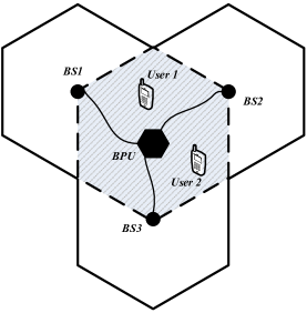
Figure 1: A network MIMO system with a 3 sector cluster.

II-B Receiver Types

At the receiver, the $n_{R}$ distributed antennas perform linear combining. Hence, the output of the combiner is $\tilde{\mbox{\boldsymbol{$r$}}}=\mbox{\boldsymbol{$W$}}^{H}\mbox{\boldsymbol{$r$}}$, where $W$ is an $n_{R}\times 2$ weight matrix. The form of $W$ and the resulting output SINR/SNR are well known for MMSE and ZF receivers. These results are summarized below. Without loss of generality, we assume that the index of the desired user is $i=1$ and we denote the first column of $W$ by $\mbox{\boldsymbol{$w$}}_{1}$. In practice, user 1 is the desired user with user 2 the interferer, followed by user 2 being detected in the presence of interference from user 1. From [11, 13, 15] the combining vector and output SINR of the MMSE receiver are given by

$$\mbox{\boldsymbol{$w$}}_{1}=\mbox{\boldsymbol{$R$}}^{-1}\mbox{\boldsymbol{$h$}}_{1},$$ (2)

$$\mbox{SINR}=\mbox{\boldsymbol{$h$}}_{1}^{H}\mbox{\boldsymbol{$R$}}^{-1}\mbox{\boldsymbol{$h$}}_{1},$$ (3)

where $\mbox{\boldsymbol{$R$}}=\mbox{\boldsymbol{$h$}}_{2}\mbox{\boldsymbol{$h$}}_{2}^{H}+\sigma^{2}\mbox{\boldsymbol{$I$}}$ and $\mbox{\boldsymbol{$h$}}_{1},\mbox{\boldsymbol{$h$}}_{2}$ denote columns 1 and 2 of $H$. From [13, 14] the combining matrix $\mbox{\boldsymbol{$W$}}=\mbox{\boldsymbol{$H$}}\left(\mbox{\boldsymbol{$H$}}^{H}\mbox{\boldsymbol{$H$}}\right)^{-1}$ and output SNR of the ZF receiver for $n_{R}\geq 2$ are given by

$$\mbox{SNR}=\frac{1}{\sigma^{2}\left[\left(\mbox{\boldsymbol{$H$}}^{H}\mbox{\boldsymbol{$H$}}\right)^{-1}\right]_{11}},$$ (4)

where $\left[\mbox{\boldsymbol{$B$}}\right]_{11}$ indicates the $\left(1,1\right)^{th}$ element of matrix $B$.

III System Analysis

In this section, we derive the CDFs of the output SINR/SNR of MMSE and ZF receivers. First, we present some useful results as follows.

III-A ZF Analysis

Let $\tilde{Z}$ be the output SNR of a ZF receiver as given in (4). $\tilde{Z}$ can be written as [15]

$$\tilde{Z} =\frac{1}{\sigma^{2}}\mbox{\boldsymbol{$h$}}_{1}^{H}\mbox{\boldsymbol{$M$}}\mbox{\boldsymbol{$h$}}_{1},$$ (5)

where $\mbox{\boldsymbol{$M$}}=\mbox{\boldsymbol{$I$}}-\mbox{\boldsymbol{$h$}}_{2}\left(\mbox{\boldsymbol{$h$}}_{2}^{H}\mbox{\boldsymbol{$h$}}_{2}\right)^{-1}\mbox{\boldsymbol{$h$}}^{H}_{2}$. The characteristic function (cf) of $\tilde{Z}$ is [20, 25]

$$\phi_{\tilde{Z}}(t) = E\left\{e^{jt\tilde{Z}}\right\}=E\left\{e^{\frac{jt}{\sigma^{2}}\mbox{\boldsymbol{$h$}}_{1}^{H}\mbox{\boldsymbol{$M$}}\mbox{\boldsymbol{$h$}}_{1}}\right\}.$$ (6)

Note that $M$ and $\mbox{\boldsymbol{$h$}}_{1}$ are independent and the pdfs of $\mbox{\boldsymbol{$h$}}_{1}$ and $\mbox{\boldsymbol{$h$}}_{2}$ are given by

$$f(\mbox{\boldsymbol{$h$}}_{k})=\frac{1}{\pi^{n_{R}}\left|\mbox{\boldsymbol{$P$}}_{k}\right|}e^{-\mbox{\boldsymbol{$h$}}_{k}^{H}\mbox{\boldsymbol{$P$}}_{k}^{-1}\mbox{\boldsymbol{$h$}}_{k}},\hskip 8.53581pt\mbox{for}\hskip 8.53581ptk=1,2,$$ (7)

where the $n_{R}\times n_{R}$ matrix $\mbox{\boldsymbol{$P$}}_{k}=\mbox{diag}(P_{1k},P_{2,k},\dots,P_{n_{R},k})$. Next, by using Lemma 2, the cf conditioned on $\mbox{\boldsymbol{$h$}}_{2}$ becomes

$$\phi_{\tilde{Z}}(t|\mbox{\boldsymbol{$h$}}_{2})=\frac{1}{\left|\mbox{\boldsymbol{$I$}}-jt\frac{1}{\sigma^{2}}\mbox{\boldsymbol{$M$}}\mbox{\boldsymbol{$P$}}_{1}\right|}.$$ (8)

Substituting $M$ in (8) and rearranging gives

$$\phi_{\tilde{Z}}(t|\mbox{\boldsymbol{$h$}}_{2})=\frac{\mbox{\boldsymbol{$h$}}^{H}_{2}\mbox{\boldsymbol{$h$}}_{2}}{\left|\mbox{\boldsymbol{$D$}}\right|\left(\mbox{\boldsymbol{$h$}}^{H}_{2}\mbox{\boldsymbol{$D$}}^{-1}\mbox{\boldsymbol{$h$}}_{2}\right)},$$ (9)

where $\mbox{\boldsymbol{$D$}}=\mbox{\boldsymbol{$I$}}-\frac{1}{\sigma^{2}}jt\mbox{\boldsymbol{$P$}}_{1}$. In Appendix B, the full cf is obtained by averaging the conditional cf in (9) over $\mbox{\boldsymbol{$h$}}_{2}$. Then, the resulting cf is inverted to give the final result, the cdf in (10). In (10), the coefficients, $\tilde{\varphi}_{ik}$, $\tilde{\psi}_{ik}$ and $\tilde{\omega}_{ik}$ are defined in (73) and the arguments, $\tilde{n}_{ik}$, $\tilde{\alpha}_{ik}$, $\tilde{m}_{ik}$ and $\tilde{\beta}_{ik}$ are defined in (65). The integrals, $\tilde{I}_{1}\left(.\right)$, $\tilde{I}_{2}\left(.\right)$ and $\tilde{I}_{3}\left(.\right)$ are given in (74)-(76).

$$F_{\tilde{Z}}(z)=\sigma^{2}\sum_{i=1}^{n_{R}}\sum_{k\neq i}^{n_{R}}\tilde{\varphi}_{ik}\tilde{I}_{1}\left(\tilde{n}_{ik},\tilde{\alpha}_{i},\tilde{m}_{ik},\tilde{\beta}_{i},z\right)+\tilde{\psi}_{ik}\tilde{I}_{2}\left(\tilde{n}_{ik},\tilde{\alpha}_{i},\tilde{m}_{ik},\tilde{\beta}_{i},z\right)+\tilde{\omega}_{ik}\tilde{I}_{3}\left(\tilde{n}_{ik},\tilde{\alpha}_{i},\tilde{m}_{ik},\tilde{\beta}_{i},z\right).$$ (10)

$$\tilde{I}_{1}\left(a,b,c,d,x\right)=\frac{1}{bc-ad}\left[\ln\left(\frac{bc}{ad}\right)-e^{-bx}e^{\frac{adx}{c}}E_{1}\left(\frac{adx}{c}\right)+E_{1}\left(bx\right)\right],$$ (11)

$$\tilde{I}_{2}\left(a,b,c,d,x\right)=\left[\frac{dx}{c\left(bc-ad\right)}+\frac{d}{\left(bc-ad\right)^{2}}\right]e^{-bx}e^{\frac{adx}{c}}E_{1}\left(\frac{adx}{c}\right)-\frac{d}{\left(bc-ad\right)^{2}}E_{1}\left(bx\right)-\frac{d+b\left(bc-ad\right)}{\left(bc-ad\right)^{2}}\ln\left(\frac{bc}{ad}\right)$$

$$+\frac{1-e^{-bx}}{a\left(bc-ad\right)},$$ (12)

$$\tilde{I}_{3}\left(a,b,c,d,x\right)=\left[\frac{ax}{c\left(bc-ad\right)}+\frac{a}{\left(bc-ad\right)^{2}}\right]e^{-bx}e^{\frac{adx}{c}}E_{1}\left(\frac{adx}{c}\right)-\frac{a}{\left(bc-ad\right)^{2}}E_{1}\left(bx\right)-\frac{a}{\left(bc-ad\right)^{2}}\ln\left(\frac{bc}{ad}\right)$$

$$+\frac{a\left(1-e^{-bx}\right)}{bc\left(bc-ad\right)}+\frac{1-e^{-bx}}{bcd}.$$ (13)

III-B MMSE Analysis

The complete MMSE analysis can be found in [26]. In this paper, we repeat a few of the initial steps which are also needed for the later high SNR results. Let Z be the output SINR of an MMSE receiver given by (3). The cf of Z is given by [11, 25]

$$\phi_{Z}(t) = E\left\{e^{jtZ}\right\}=E\left\{e^{jt\mbox{\boldsymbol{$h$}}_{1}^{H}\mbox{\boldsymbol{$R$}}^{-1}\mbox{\boldsymbol{$h$}}_{1}}\right\}.$$ (14)

As in the ZF analysis, we first obtain the cf conditioned on $\mbox{\boldsymbol{$h$}}_{2}$. The conditional cf is given by

$$\phi_{Z}(t|\mbox{\boldsymbol{$h$}}_{2})=\frac{1}{\left|\mbox{\boldsymbol{$I$}}-jt\mbox{\boldsymbol{$R$}}^{-1}\mbox{\boldsymbol{$P$}}_{1}\right|}.$$ (15)

Substituting $R$ in (15) and rearranging gives

$$\phi_{Z}(t|\mbox{\boldsymbol{$h$}}_{2})=\frac{\sigma^{2}+\mbox{\boldsymbol{$h$}}_{2}^{H}\mbox{\boldsymbol{$h$}}_{2}}{\left|\mbox{\boldsymbol{$D$}}\right|\left(\sigma^{2}+\mbox{\boldsymbol{$h$}}_{2}^{H}\mbox{\boldsymbol{$D$}}^{-1}\mbox{\boldsymbol{$h$}}_{2}\right)}.$$ (16)

Comparing $(\ref{eq:zf:cf3})$ with $(\ref{eq:mmse:cf3})$ we observe that, as expected, the MMSE results converge to the ZF results as $\sigma^{2}\rightarrow 0$. Again, Lemma 1 can be used to average the conditional cf in (16) to obtain the unconditional cf and in turn the cdf of the output SINR of an MMSE receiver as in [26]. For the sake of completeness, we give the final results in (17)-(20).

$$F_{Z}(z)=\sigma^{2}\sum_{i=1}^{n_{R}}\sum_{k\neq i}^{n_{R}}\varphi_{ik}I_{1}\left(\sigma^{2}\tilde{n}_{ik},\tilde{\alpha}_{i},\tilde{m}_{ik},\frac{\tilde{\beta}_{i}}{\sigma^{2}},z\right)+\psi_{ik}I_{2}\left(\sigma^{2}\tilde{n}_{ik},\tilde{\alpha}_{i},\tilde{m}_{ik},\frac{\tilde{\beta}_{i}}{\sigma^{2}},z\right)+\omega_{ik}I_{3}\left(\sigma^{2}\tilde{n}_{ik},\tilde{\alpha}_{i},\tilde{m}_{ik},\frac{\tilde{\beta}_{i}}{\sigma^{2}},z\right).$$ (17)

$$I_{1}\left(a,b,c,d,x\right) =\frac{1}{bc-ad}\left[e^{\frac{a}{c}}E_{1}\left(\frac{a}{c}\right)-e^{\frac{b}{d}}E_{1}\left(\frac{b}{d}\right)+e^{\frac{b}{d}}E_{1}\left(\frac{b}{d}+bx\right)-e^{-bx}e^{\frac{\left(1+dx\right)a}{c}}E_{1}\left(\frac{\left(1+dx\right)a}{c}\right)\right].$$ (18)

$$I_{2}\left(a,b,c,d,x\right)=\left[\frac{d}{\left(bc-ad\right)^{2}}+\frac{1+dx}{c\left(bc-ad\right)}\right]e^{-bx}e^{\frac{\left(1+dx\right)a}{c}}E_{1}\left(\frac{\left(1+dx\right)a}{c}\right)-\left.\frac{cd+bc-ad}{c\left(bc-ad\right)^{2}}\right.e^{\frac{a}{c}}E_{1}\left(\frac{a}{c}\right)$$

$$+\frac{d}{\left(bc-ad\right)^{2}}e^{\frac{b}{d}}\left[E_{1}\left(\frac{b}{d}\right)-E_{1}\left(\frac{b}{d}+bx\right)\right]+\frac{1-e^{-bx}}{a\left(bc-ad\right)}.$$ (19)

$$I_{3}\left(a,b,c,d,x\right)=\left[\frac{a}{\left(bc-ad\right)^{2}}+\frac{ax}{c\left(bc-ad\right)}\right]e^{-bx}e^{\frac{\left(1+dx\right)a}{c}}E_{1}\left(\frac{\left(1+dx\right)a}{c}\right)+\left.\frac{\left.ad^{2}+abd-b^{2}c\right.}{d^{2}\left(bc-ad\right)^{2}}\right.e^{\frac{b}{d}}\left[E_{1}\left(\frac{b}{d}\right)\right.$$

$$\left.-E_{1}\left(\frac{b}{d}+bx\right)\right]-\frac{a}{\left(bc-ad\right)^{2}}e^{\frac{a}{c}}E_{1}\left(\frac{a}{c}\right)+\frac{1-e^{-bx}}{d\left(bc-ad\right)}.$$ (20)

^∗Results pertaining to MMSE receiver.

The cdf is defined in (17) in terms of $I_{1}\left(.\right)$, $I_{2}\left(.\right)$ and $I_{3}\left(.\right)$ which are given in (18)-(20). Finally, the necessary constants $\varphi_{ik}$, $\psi_{ik}$ and $\omega_{ik}$ are given by

$$\!\!\!\!\varphi_{ik}\! =\!P_{i1}^{n_{R}-2}\!\left(\sigma^{2}\tilde{\eta}_{ik}\!+\!\tilde{\Delta}_{i}\tilde{\eta}_{ik}\!+\!\tilde{\zeta}_{ik}-(n_{R}-2)P_{i2}\tilde{\eta}_{ik}\right),$$ (21a)

$$\psi_{ik} =\sigma^{2}P_{i1}^{n_{R}-2}\tilde{\eta}_{ik}\tilde{\xi}_{ik},$$ (21b)

$$\omega_{ik} =-P_{i2}^{2}P_{i1}^{n_{R}-3}\tilde{\eta}_{ik}.$$ (21c)

IV SER Approximations

In this section, we derive high SNR approximations for the SER of MMSE and ZF receivers. This is motivated by the complexity of the exact analysis and the importance of finding a simple, functional link between performance and the average link SNRs.

IV-A ZF Analysis

The conditional cf in (9) is a ratio of quadratic forms in $\mbox{\boldsymbol{$h$}}_{2}$. Hence, $\phi_{\tilde{Z}}(t)=E\{\phi_{\tilde{Z}}(t|\mbox{\boldsymbol{$h$}}_{2})\}$ is the mean of a ratio of quadratic forms which can be approximated by the Laplace approximation [27] as

$$\phi_{\tilde{Z}}(t)\approx\frac{E\{\mbox{\boldsymbol{$h$}}^{H}_{2}\mbox{\boldsymbol{$h$}}_{2}\}}{\left|\mbox{\boldsymbol{$D$}}\right|E\left\{\mbox{\boldsymbol{$h$}}^{H}_{2}\mbox{\boldsymbol{$D$}}^{-1}\mbox{\boldsymbol{$h$}}_{2}\right\}}=\frac{\mbox{Tr}\left(\mbox{\boldsymbol{$P$}}_{2}\right)}{|\mbox{\boldsymbol{$D$}}|\mbox{Tr}\left(\mbox{\boldsymbol{$D$}}^{-1}\mbox{\boldsymbol{$P$}}_{2}\right)}.$$ (22)

Note that the second equality in (22) follows from the result, $E\{\mbox{\boldsymbol{$u$}}^{H}\mbox{\boldsymbol{$Q$}}\mbox{\boldsymbol{$u$}}\}=\mbox{Tr}\left(\mbox{\boldsymbol{$Q$}}\right)$, where $\mbox{\boldsymbol{$u$}}\sim\mathcal{CN}\left(0,\mbox{\boldsymbol{$I$}}\right)$ and $Q$ is a Hermitian matrix. Expanding the denominator of (22) gives

$$\phi_{\tilde{Z}}(t)\approx\frac{\mbox{Tr}\left(\mbox{\boldsymbol{$P$}}_{2}\right)}{\sum_{i=1}^{n_{R}}P_{i2}\prod_{k\neq i}^{n_{R}}\left(1-\frac{jt}{\sigma^{2}}P_{k1}\right)},$$ (23)

which follows since $D$ and $\mbox{\boldsymbol{$P$}}_{2}$ are diagonal and $\left|\mbox{\boldsymbol{$D$}}\right|$ is the product of the diagonal entries of $D$. As the SNR grows, $\sigma^{2}\rightarrow 0$ and keeping only the dominant power of $\sigma^{2}$ in (23) gives

$$\phi_{\tilde{Z}}(t)\approx\left.\frac{\mbox{Tr}\left(\mbox{\boldsymbol{$P$}}_{2}\right)}{\left|\mbox{\boldsymbol{$P$}}_{1}\right|\mbox{Tr}\left(\mbox{\boldsymbol{$P$}}_{1}^{-1}\mbox{\boldsymbol{$P$}}_{2}\right)}\right.\frac{\sigma^{2\left(n_{R}-1\right)}}{\left(-jt\right)^{n_{R}-1}}.$$ (24)

Defining $\vartheta\left(\mbox{\boldsymbol{$P$}}_{1},\mbox{\boldsymbol{$P$}}_{2}\right)=\frac{\mbox{Tr}\left.\mbox{\boldsymbol{$P$}}_{2}\right.}{\left|\mbox{\boldsymbol{$P$}}_{1}\right|\mbox{Tr}\left(\mbox{\boldsymbol{$P$}}_{1}^{-1}\mbox{\boldsymbol{$P$}}_{2}\right)}$ gives a metric which encapsulates the effects of the power matrices $\mbox{\boldsymbol{$P$}}_{1}$ and $\mbox{\boldsymbol{$P$}}_{2}$. For many modulations, the SER can be evaluated as a single integral of the moment generating function of the SNR [28]. The mgf of the SNR is $\mathcal{M}_{\tilde{Z}}\left(s\right)=\phi_{\tilde{Z}}\left(-js\right)$. As an example, for MPSK the SER is [28, 29]

$$\tilde{P}_{s}=\frac{1}{\pi}\int_{0}^{T}\mathcal{M}_{\tilde{Z}}\left(-\frac{g}{\sin^{2}\theta}\right)d\theta,$$ (25)

where $g=\sin^{2}\left(\pi/M\right)$ and $T=\frac{\left(M-1\right)\pi}{M}$. Substituting (24) in (25) gives the approximation

$$\tilde{P}_{s}\approx\left(\tilde{G}_{a}\bar{\gamma}\right)^{-\tilde{G}_{d}}.$$ (26)

In (26), the average SNR is $\bar{\gamma}=\frac{1}{\sigma^{2}}$, and the diversity gain and array gain are given by

$$\tilde{G}_{d}=n_{R}-1,\hskip 28.45274pt\tilde{G}_{a}=\left(\vartheta\left(\mbox{\boldsymbol{$P$}}_{1},\mbox{\boldsymbol{$P$}}_{2}\right)\tilde{\mathcal{I}}\right)^{-1/(n_{R}-1)}.$$

The constant integral, $\tilde{\mathcal{I}}$, is given by

$$\tilde{\mathcal{I}}=\frac{1}{\pi}\int_{0}^{T}\left(\frac{\sin^{2}\theta}{g}\right)^{\left.n_{R}-1\right.}d\theta.$$ (27)

Note that the simple representation in (26) shows the diversity order of $n_{R}-1$ and the effect of the link powers on array gain controlled by the metric $\vartheta\left(\mbox{\boldsymbol{$P$}}_{1},\mbox{\boldsymbol{$P$}}_{2}\right)$. The integral $\tilde{\mathcal{I}}$ can be solved in closed form and the final result is given in (28).

$$\tilde{\mathcal{I}}=\frac{1}{\pi g^{\left.n_{R}-1\right.}}\left\{\frac{T}{2^{2\left(n_{R}-1\right)}}\left(\frac{2n_{R}-2}{n_{R}-1}\right)+\frac{(-1)^{n_{R}-1}}{2^{2n_{R}-3}}\sum_{k=0}^{n_{R}-2}(-1)^{k}\left(\frac{2n_{R}-2}{k}\right)\frac{\sin\left(2\left(n_{R}-k-1\right)T\right)}{2\left(n_{R}-k-1\right)}\right\},$$ (28)

IV-B MMSE Analysis

By using the Laplace approximation for the expectation of the conditional cf in (16), we obtain

$$\phi_{Z}(t)\approx\frac{\sigma^{2}+\mbox{Tr}\left(\mbox{\boldsymbol{$P$}}_{2}\right)}{|\mbox{\boldsymbol{$D$}}|\left(\sigma^{2}+\mbox{Tr}\left(\mbox{\boldsymbol{$D$}}^{-1}\mbox{\boldsymbol{$P$}}_{2}\right)\right)}.$$ (29)

As the SNR grows, $\sigma^{2}\rightarrow 0$ and keeping only the dominant power of $\sigma^{2}$ in (29) gives

$$\phi_{Z}(t)\approx\frac{\mbox{Tr}\left(\mbox{\boldsymbol{$P$}}_{2}\right)\left(\frac{1}{-jt\bar{\gamma}}\right)^{n_{R}-1}}{\left|\mbox{\boldsymbol{$P$}}_{1}\right|\left(\mbox{Tr}\left(\mbox{\boldsymbol{$P$}}_{1}^{-1}\mbox{\boldsymbol{$P$}}_{2}\right)-jt\right)}.$$ (30)

As in the ZF analysis, the SER for MPSK can be approximated by

$$P_{s}\approx\left(G_{a}\bar{\gamma}\right)^{-G_{d}},$$ (31)

where the diversity gain and array gain are given by

$$G_{d} =n_{R}-1,\hskip 42.67912ptG_{a}=\left(\vartheta\left(\mbox{\boldsymbol{$P$}}_{1},\mbox{\boldsymbol{$P$}}_{2}\right)\mathcal{I}\left(\mbox{\boldsymbol{$P$}}_{1},\mbox{\boldsymbol{$P$}}_{2}\right)\right)^{-1/(n_{R}-1)}.$$ (32)

In (32), $\mathcal{I}\left(\mbox{\boldsymbol{$P$}}_{1},\mbox{\boldsymbol{$P$}}_{2}\right)$ is given by

$$\mathcal{I}\left(\mbox{\boldsymbol{$P$}}_{1},\mbox{\boldsymbol{$P$}}_{2}\right)=\frac{1}{\pi}\int_{0}^{T}\frac{g^{-\left(n_{R}-1\right)}\sin^{2n_{R}}\theta}{g_{0}+\sin^{2}\theta}d\theta,$$ (33)

where $g=g_{0}\mbox{Tr}\left(\mbox{\boldsymbol{$P$}}_{1}^{-1}\mbox{\boldsymbol{$P$}}_{2}\right)$. The integral, $\mathcal{I}\left(\mbox{\boldsymbol{$P$}}_{1},\mbox{\boldsymbol{$P$}}_{2}\right)$, can be solved in closed form by expanding the ratio of $\sin^{2}\theta$ terms in (33) as a polynomial and integrating term by term to get the final result in (34).

$$\begin{split}\mathcal{I}\left(\mbox{\boldsymbol{$P$}}_{1},\mbox{\boldsymbol{$P$}}_{2}\right)&=\left(-1\right)^{n_{R}}\frac{g_{0}^{n_{R}-1}}{\pi g^{n_{R}-1}}\left\{\sqrt{\frac{g_{0}}{1+g_{0}}}\tan^{-1}\left(\sqrt{\frac{1+g_{0}}{g_{0}}}\tan T\right)-\sum_{i=0}^{n_{R}-1}(-1)^{i}\frac{1}{g_{0}^{i}}\right.\\ &\times\left.\left[\frac{T}{2^{2i}}\left(\frac{2i}{i}\right)+\frac{(-1)^{i}}{2^{2i-1}}\sum_{k=0}^{i-1}(-1)^{k}\left(\frac{2i}{k}\right)\frac{\sin\left(2\left(i-k\right)T\right)}{2\left(i-k\right)}\right]\right\}.\end{split}$$ (34)

We note that, as expected, the diversity order of $n_{R}-1$ is observed in both receiver types and the difference only appears in the array gains.
The approximate, high SNR result for ZF in (26) is particularly useful since it is simpler than the MMSE version in (31), and at high SNR the performance of the two schemes is similar anyway. Hence, (26) acts as a useful approximation for both ZF and MMSE and provides a remarkably compact relationship between SER and the link powers, via the single function, $\vartheta\left(\mbox{\boldsymbol{$P$}}_{1},\mbox{\boldsymbol{$P$}}_{2}\right)$.

V High SNR Analysis

In this section, we derive exact high SNR results for the SER of MMSE and ZF receivers. The work in this section does not employ the Laplace type approximation used in (22) and (29) and hence produces exact asymptotics at the expense of increased complexity. The mathematical details are given in brief to avoid unnecessary detail.

V-A ZF Analysis

The conditional cf in (9) is a ratio of quadratic forms in $\mbox{\boldsymbol{$h$}}_{2}$. As the SNR grows, $\sigma^{2}\rightarrow 0$ and keeping only the dominant power of $\sigma^{2}$ in (9) gives

$$\phi_{\tilde{Z}}(t|\mbox{\boldsymbol{$h$}}_{2})\approx\frac{\mbox{\boldsymbol{$h$}}^{H}_{2}\mbox{\boldsymbol{$h$}}_{2}}{|\mbox{\boldsymbol{$P$}}_{1}|\left(\mbox{\boldsymbol{$h$}}^{H}_{2}\mbox{\boldsymbol{$P$}}_{1}^{-1}\mbox{\boldsymbol{$h$}}_{2}\right)}\left(\frac{\sigma^{2}}{-jt}\right)^{n_{R}-1}.$$ (35)

Hence, the unconditional cf, when $\sigma^{2}\rightarrow 0$, becomes

$$\phi_{\tilde{Z}}(t)=\tilde{K}_{0}\left(\frac{\sigma^{2}}{-jt}\right)^{n_{R}-1}+o\left(\sigma^{2\left(n_{R}-1\right)}\right),$$ (36)

where $o\left(.\right)$ is the standard ”little-o” notation and represents the fact that only the dominant power of $\sigma^{2}$ is used in the approximation and

$$\tilde{K}_{0}=\frac{1}{|\mbox{\boldsymbol{$P$}}_{1}|}E\left\{\frac{\mbox{\boldsymbol{$h$}}^{H}_{2}\mbox{\boldsymbol{$h$}}_{2}}{\left.\mbox{\boldsymbol{$h$}}^{H}_{2}\mbox{\boldsymbol{$P$}}_{1}^{-1}\mbox{\boldsymbol{$h$}}_{2}\right.}\right\}.$$ (37)

Following the same mgf based procedure to obtain the SER as in Sec. IV, we arrive at the following expression

$$\tilde{P}_{s}=\left(\tilde{G}_{ea}\bar{\gamma}\right)^{-\tilde{G}_{ed}}+o\left(\bar{\gamma}^{-\tilde{G}_{ed}}\right),$$ (38)

where, the diversity and array gains are given by

$$\tilde{G}_{ed}=n_{R}-1,\hskip 28.45274pt\tilde{G}_{ea}=\left(\tilde{K}_{0}\tilde{\mathcal{I}}\right)^{-1/(n_{R}-1)}.$$

The constant, $\tilde{K}_{0}$, can be found using Lemma 1 to obtain the final expression as in (39)

$$\begin{split}\tilde{K}_{0}=\sum_{i=1}^{n_{R}}\Upsilon_{i}P_{i2}+\sum_{1\leq u\neq v\leq n_{R}}^{n_{R}}\left(\Upsilon_{u}P_{v1}+\Upsilon_{v}P_{u1}\right)\left(\frac{\ln\left(\frac{P_{u1}}{P_{u2}}\right)-\ln\left(\frac{P_{v1}}{P_{v2}}\right)}{\frac{P_{u1}}{P_{u2}}-\frac{P_{v1}}{P_{v2}}}\right)\end{split}$$ (39)

where

$$\Upsilon_{i} =\frac{P_{i2}^{n_{R}-2}}{\prod_{k\neq i}^{n_{R}}P_{k1}P_{i2}-P_{i1}P_{k2}}.$$ (40)

V-B MMSE Analysis

Consider the expectation of the conditional cf expression in (16). As the SNR grows, $\sigma^{2}\rightarrow 0$ and keeping only the dominant power of $\sigma^{2}$ in (16) gives

$$\phi_{Z}(t)=K_{0}\left(jt\right)\left(\frac{\sigma^{2}}{-jt}\right)^{n_{R}-1}+o\left(\sigma^{2\left(n_{R}-1\right)}\right),$$ (41)

where

$$K_{0}\left(s\right)=\frac{1}{|\mbox{\boldsymbol{$P$}}_{1}|}E\left\{\frac{\mbox{\boldsymbol{$h$}}_{2}^{H}\mbox{\boldsymbol{$h$}}_{2}}{\left.\mbox{\boldsymbol{$h$}}_{2}^{H}\mbox{\boldsymbol{$P$}}_{1}^{-1}\mbox{\boldsymbol{$h$}}_{2}-s\right.}\right\}.$$ (42)

Following the mgf based procedure in Sec. IV, the SER at high SNR becomes

$$P_{s}\approx\frac{1}{\pi}\int_{0}^{T}\left(\frac{\sigma^{2}\sin^{2}\theta}{g}\right)^{n_{R}-1}K_{0}\left(-\frac{g}{\sin^{2}\theta}\right)d\theta.$$ (43)

From (43), the approximate SER can be written in terms of the diversity gain and array gain as

$$P_{s}=\left(G_{ea}\bar{\gamma}\right)^{-G_{ed}}+o\left(\bar{\gamma}^{-G_{ed}}\right),$$ (44)

where

$$G_{ed}=n_{R}-1,\hskip 28.45274ptG_{ea}=\left(\mathcal{I}_{e}\left(\mbox{\boldsymbol{$P$}}_{1},\mbox{\boldsymbol{$P$}}_{2}\right)\right)^{-1/(n_{R}-1)},$$

$$\mathcal{I}_{e}\left(\mbox{\boldsymbol{$P$}}_{1},\mbox{\boldsymbol{$P$}}_{2}\right)\!=\!\frac{1}{\pi}\int_{0}^{T}\!\!\!\left(\!\frac{\sin^{2}\theta}{g}\!\right)^{n_{R}-1}\!\!\!\!K_{0}\left(-\frac{g}{\sin^{2}\theta}\right)d\theta.$$ (45)

Using Lemma 1, $K_{0}\left(-s\right)$ can be given by

$$K_{0}\left(-s\right)=-\int_{0}^{\infty}\frac{\partial}{\partial\theta_{1}}\left[\frac{e^{-s\theta_{2}}}{|\mbox{\boldsymbol{$P$}}_{1}+\theta_{1}\mbox{\boldsymbol{$P$}}_{2}\mbox{\boldsymbol{$P$}}_{1}+\theta_{2}\mbox{\boldsymbol{$P$}}_{2}|}\right]_{\theta_{1}=0}d\theta_{2},$$ (46)

which can be simplified to obtain

$$\begin{split}K_{0}\left(-s\right)=\int_{0}^{\infty}e^{-s\theta_{2}}&\left(\sum_{i=1}^{n_{R}}\frac{P_{i2}\Upsilon_{i}}{P_{i2}\theta_{2}+P_{i1}}\right)\left(\sum_{i=1}^{n_{R}}\frac{P_{i1}P_{i2}}{P_{i2}\theta_{2}+P_{i1}}\right)d\theta_{2},\end{split}$$ (47)

where $\Upsilon_{i}$ is given in (40). Equation (47) can be solved in closed form to give

$$\begin{split}K_{0}\left(-s\right)\!=\!\sum_{i=1}^{n_{R}}\left\{e^{s\frac{P_{i1}}{P_{i2}}}E_{1}\left(s\frac{P_{i1}}{P_{i2}}\right)\!\!\left(\Phi_{i}-s\Upsilon_{i}P_{i1}\right)+\Upsilon_{i}P_{i2}\right\},\end{split}$$ (48)

where

$$\begin{split}\Phi_{i}&=\sum_{k\neq i}^{n_{R}}\frac{P_{i2}\Upsilon_{i}P_{k1}P_{k2}+P_{k2}\Upsilon_{k}P_{i1}P_{i2}}{P_{k1}P_{i2}-P_{k2}P_{i1}}.\end{split}$$ (49)

Substituting $s=g/\sin^{2}\theta$ in (48) and then substituting $K_{0}\left(-\frac{g}{\sin^{2}\theta}\right)$ in (45) and integrating over $\theta$ gives the result in (50)

$$\begin{split}\mathcal{I}_{e}\left(\mbox{\boldsymbol{$P$}}_{1},\mbox{\boldsymbol{$P$}}_{2}\right)=\tilde{\mathcal{I}}\left(\sum_{i=1}^{n_{R}}\Upsilon_{i}P_{i2}\right)+\frac{1}{\pi g^{\left.n_{R}-1\right.}}\sum_{i=1}^{n_{R}}\left\{\Phi_{i}H\left(n_{R}-1,g\frac{P_{i1}}{P_{i2}}\right)-\Upsilon_{i}P_{i1}H\left(n_{R}-2,g\frac{P_{i1}}{P_{i2}}\right)\right\}\end{split}$$ (50)

where

$$\begin{split}H\left(m,a\right)=\int_{0}^{T}e^{\frac{a}{\sin^{2}\theta}}E_{1}\left(\frac{a}{\sin^{2}\theta}\right)\left.\sin^{2m}\theta\right.d\theta.\end{split}$$ (51)

Clearly the exact asymptotics, especially for the MMSE case, are substantially more complex than the approximations in Sec. IV. Also, the relationship between SER and the link powers is far more involved.

VI Numerical Results

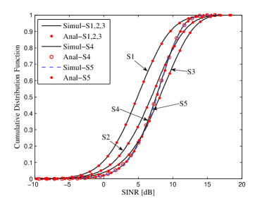
Figure 2: Analytical and simulated cdfs for the output SINR of an MMSE receiver for scenarios S1-S5 listed in Table 1 at $\rho=5$ dB with $\varsigma=1$.

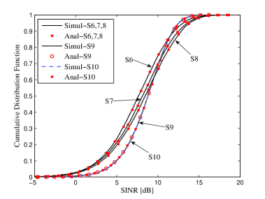
Figure 3: Analytical and simulated cdfs for the output SINR of an MMSE receiver for scenarios S6-S10 listed in Table 1 at $\rho=5$ dB with $\varsigma=20$.

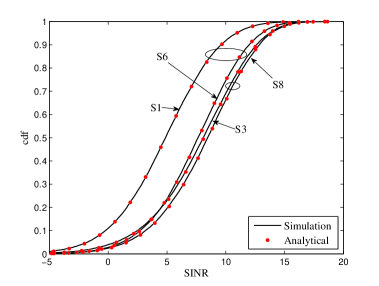
Figure 4: Analytical and simulated cdfs for the output SINR of an MMSE receiver for scenarios (S1,S6) and (S3,S8) in Table 1.

TABLE I: Parameters for Figures 2 and 3

	Decay Parameter
Sc. No.	Desired	Interfering	$\varsigma$
S1	$\alpha=0.2$	$\alpha=0.2$	1
S2	$\alpha=0.2$	$\alpha=1$	1
S3	$\alpha=0.2$	$\alpha=5$	1
S4	$\alpha=1$	$\alpha=1$	1
S5	$\alpha=1$	$\alpha=0.2$	1
S6	$\alpha=0.2$	$\alpha=0.2$	20
S7	$\alpha=0.2$	$\alpha=1$	20
S8	$\alpha=0.2$	$\alpha=5$	20
S9	$\alpha=1$	$\alpha=1$	20
S10	$\alpha=1$	$\alpha=0.2$	20

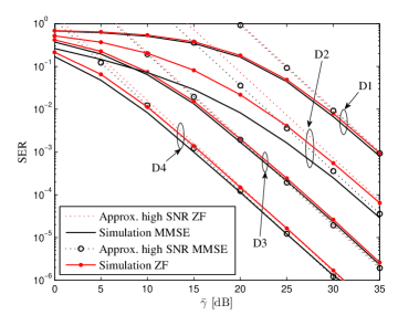
Figure 5: SER and high SNR approximations for MMSE/ZF receivers using QPSK modulation in flat Rayleigh fading for four arbitrary drops.

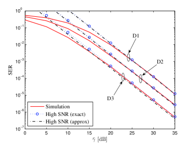
Figure 6: SER of a ZF receiver using QPSK modulation in Rayleigh flat fading for three arbitrary drops.

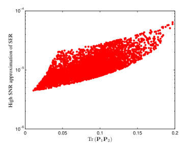
Figure 7: SER of a MMSE receiver for QPSK modulation in flat Rayleigh fading at $\bar{\gamma}=35$ dB.

In this section, we verify the analysis by Monte Carlo simulations using the network MIMO scenario in Fig. 1 [26]. We also consider some special cases of $\mbox{\boldsymbol{$P$}}_{1}$ and $\mbox{\boldsymbol{$P$}}_{2}$ in order to investigate the effect of the macrodiversity powers on performance. For the two-user system in Fig. 1, we consider the desired user to be user 1 and parameterize the system by three parameters. The average received signal to noise ratio is defined by $\rho=\left.\mbox{Tr}\left(\mbox{\boldsymbol{$P$}}_{1}\right)\right./n_{R}\sigma^{2}$. The total signal to interference ratio is defined by $\varsigma=\mbox{Tr}\left(\mbox{\boldsymbol{$P$}}_{1}\right)/\mbox{Tr}\left(\mbox{\boldsymbol{$P$}}_{2}\right)$. The spread of the signal power across the three antennas is assumed to follow an exponential profile, as in [11], so that a range of possibilities can be covered with only one parameter. The exponential profile is defined by

$$P_{ik} =K_{k}\left(\alpha\right)\alpha^{i-1},$$ (52)

for receive antenna i, source k where

$$K_{k}\left(\alpha\right) =\mbox{Tr}\left(\mbox{\boldsymbol{$P$}}_{k}\right)/\left(1+\alpha+\alpha^{2}\right),\quad k=1,2,$$ (53)

and $\alpha>0$ is the parameter controlling the uniformity of the powers across the antennas. Note that as $\alpha\rightarrow 0$ the received power is dominant at the first antenna, as $\alpha$ becomes large $\left(\alpha\gg 1\right)$ the third antenna is dominant and as $\alpha\rightarrow 1$ there is an even spread, as in the standard microdiversity scenario. Although we consider microdiversity (S4 and S9), this is in the context of exploring the effect of different $P$ matrix structures. Physically, it is not sensible to directly compare microdiversity with macrodiversity as they involve different system structures. In microdiversity, there may be multiple users communicating with a single array at a single BS. In macrodiversity, the users may be communicating with distributed antennas located at different BS sites which are back-hauled together to enable joint transmission/reception. In Figs. 2-3 we show cdf results for the ten scenarios given in Table I. In Fig. 2, we see that S1 has the worst cdf since the sharply decaying power profile is identical for both desired and interfering source. Hence, there is reduced diversity, as most of the signal strength is seen at one antenna, and there is strong interference at each antenna. Scenario S3 is best at high SINR since in this interference limited situation $\left(\varsigma=1\right)$ it is best to have at least one antenna where there is minimal interference. This occurs with S3 as the power profiles are opposing and the strongest desired signal aligns with the weakest interferer. At low SINR, scenarios S4 and S5 are slightly better than S3 as they have full diversity (equal power at each antenna) which is beneficial in this SINR region. In Fig. 3, similar results are observed with diversity being important at lower SINR (where S9 and S10 are the best) and interference reduction being important at high SINR (where S8 is best). In Fig. 4, we consider the effect of $\varsigma$ on two different macrodiversity scenarios in Table I. In particular, we have shown results for S1 and S6 and S3 and S8. As expected, S1 and S3 have lower SINRs than S6 and S9 due to increased interference. However, S1 is far more sensitive to $\varsigma$ than S3. This is because S3 has opposing power profiles for the desired and interfering users so that the two sources are more orthogonal and interference plays a smaller part in performance.
Next, we consider the high SNR results in Secs. IV and V. In Fig. 5, the MMSE/ZF receivers are considered for four drops (D1, D2, D3 and D4) of two users in the shaded coverage area of Fig. 1. Each user is dropped at a different random location (uniformly generated over the coverage area) and random lognormal shadow fading and path loss is considered where $\sigma_{SF}=8$dB (standard deviation of shadow fading) and $\gamma=3.5$ (path loss exponent). Hence, each user has a different distance and shadow fade to each BS and each drop results in a new $P$ matrix. The transmit power of the sources is scaled so that all locations in the coverage area have a maximum received SNR greater than $3$dB, at least $95\%$ of the time. The maximum SNR is taken over the 3 BSs. For all four drops, the high SNR approximations from Sec. IV are shown to be very accurate for SERs below $10^{-2}$, although for drop D2 the results are less tight. Note that drop D2 has the greatest difference between the MMSE and ZF results. In general, the gap between MMSE and ZF results can be assessed by a comparison of (27) with (33). Here, it can be seen that the approximate asymptotics are the same for ZF and MMSE when $g_{0}=0$. Hence, scenarios where $g_{0}$ is large, i.e., $\mbox{Tr}\left(\mbox{\boldsymbol{$P$}}_{1}^{-1}\mbox{\boldsymbol{$P$}}_{2}\right)\approx 0$, will create substantial differences between the two receivers. In Fig. 5, drop D2 had the smallest value of $\mbox{Tr}\left(\mbox{\boldsymbol{$P$}}_{1}^{-1}\mbox{\boldsymbol{$P$}}_{2}\right)$ and hence showed the greatest difference. Note that for $\mbox{Tr}\left(\mbox{\boldsymbol{$P$}}_{1}^{-1}\mbox{\boldsymbol{$P$}}_{2}\right)$ to be small, $P_{i1}\gg P_{i2}$ is required for $i=1,2,\dots,n_{R}$. Hence, the power profiles for users 1 and 2 must be “parallel” in some sense, with any large value of $P_{i2}$ aligning with an even larger value of $P_{i1}$. In these “parallel” scenarios, MMSE and ZF results can exhibit greater differences.
This methodology is used again in Fig. 6 for three drops and ZF results are shown. Again, the asymptotic results show good agreement at SERs below $10^{-2}$. Furthermore, the difference between the approximations in Sec. IV and the exact asymptotics in Sec. V is shown to be minor. Hence the simple SER forms in (26) and (31) are particularly useful. Note that the power matrices, $\mbox{\boldsymbol{$P$}}_{1}$ and $\mbox{\boldsymbol{$P$}}_{2}$, are completely general, with the sole constraint being $P_{ik}\geq 0$, $\forall i,k$. As a result, it is likely that some combinations of powers can be found that will cause the approximate SERs to lose accuracy. However, in all the scenarios considered and all random drops simulated (see also [26]) the approximations have shown similar accuracy to the results in Figs. 5 and 6.
In multiuser systems it is well-known that two users may be successfully detected if their channels are approximately orthogonal. In the context of a dual user system, where only the channel powers are considered, the analog would be that $\mbox{Tr}\left(\mbox{\boldsymbol{$P$}}_{1}\mbox{\boldsymbol{$P$}}_{2}\right)$ is small. To investigate this relationship, we generate a large number of random power matrices with a fixed total power. For user 1, the powers are generated by (52) with $\alpha=0.2$. For user 2, the powers are independent uniform random variables which are scaled so that $\varsigma=1$. For each pair, $\left(\mbox{\boldsymbol{$P$}}_{1},\mbox{\boldsymbol{$P$}}_{2}\right)$, we compute $\mbox{Tr}\left(\mbox{\boldsymbol{$P$}}_{1}\mbox{\boldsymbol{$P$}}_{2}\right)$ and the approximate SER of user 1 using using (31). The results are plotted in Fig. 7. As expected, SER increases with $\mbox{Tr}\left(\mbox{\boldsymbol{$P$}}_{1}\mbox{\boldsymbol{$P$}}_{2}\right)$, although there is wide variation in the band of SER results. In comparison, the new metric, $\vartheta\left(\mbox{\boldsymbol{$P$}}_{1},\mbox{\boldsymbol{$P$}}_{2}\right)$, has a one-to-one relationship with the approximate SER and carries far more information than ad-hoc measures such as $\mbox{Tr}\left(\mbox{\boldsymbol{$P$}}_{1}\mbox{\boldsymbol{$P$}}_{2}\right)$.

VII Conclusion

In this paper, we derived the exact cdf of the output SINR/SNR for MMSE and ZF receivers in the presence of a single interfering user with an arbitrary number of receive antennas. To the best of our knowledge, this represents the first exact analysis of linear combining in macrodiversity systems. Although not shown for reasons of space, the slightly simpler problem of obtaining the associated pdf can also be handled since the pdf expression in (58) is inherently computed en-route to the cdf in (59). Numerical examples demonstrate the validity of the analysis across arbitrary drops and channels. This suggests that the analysis is also numerically robust. A high SNR analysis reveals simple SER results for both MMSE and ZF which provide insights into both diversity and array gain. It also provides a functional link between the performance of the macrodiversity system and the link SNRs.

Appendix A Background Results

The following lemma gives a compact method to calculate the expected value of a ratio of random variables with arbitrary integer powers [23].

Lemma 1.

Let $U_{1}$, $U_{2}$ and $Z$ be three continuous random variables such that $P(U_{2}>0)=1$, $Z\geq 0$ and $Z=\frac{U_{1}^{m}}{U_{2}^{n}}$. Assuming that there exists a joint moment generating function (mgf) for $U_{1}$ and $U_{2}$, denoted $\mathcal{M}(\theta_{1},\theta_{2})=E\left(e^{\theta_{1}U_{1}+\theta_{2}U_{2}}\right)$, then, for all positive integer values of $m$ and $n$, the expected value of $Z$ is given by

$$E\left\{\frac{U_{1}^{m}}{U_{2}^{n}}\right\}=\frac{1}{(n-1)!}\int_{0}^{\infty}z^{n-1}\left.\frac{\partial^{m}\mathcal{M}(\theta,-z)}{\partial\theta^{m}}\right|_{\theta=0}dz.$$

The following n-dimensional complex Gaussian integral identity will be used extensively.

Lemma 2.

Let $A$ be an arbitrary $n\times n$ complex Hermitian positive definite matrix. Then, the following integral identity holds.

$$\int_{-\infty}^{\infty}\ldots\int_{-\infty}^{\infty}e^{-\mbox{\boldsymbol{$x$}}^{H}\mbox{\boldsymbol{$A$}}\normalsize{\mbox{\boldsymbol{$x$}}}}dx_{1}\ldots dx_{n}=\frac{\pi^{n}}{\left|\mbox{\boldsymbol{$A$}}\right|},$$

where the complex $n\times 1$ vector $\mbox{\boldsymbol{$x$}}=[x_{1},\ldots,x_{n}]^{T}$, $dx_{i}=dx_{iI}dx_{iQ}$, $x_{iI}=\textup{Re}(x_{i})$ and $x_{iQ}=\textup{Im}(x_{i})$.

Finally, we give the following partial fraction expansion from elementary algebra,

$$\frac{1}{\prod_{i=1}^{n_{R}}\left(a_{i}-jtb_{i}\right)}=\sum_{i=1}^{n_{R}}\frac{A_{i}}{\left.\frac{a_{i}}{b_{i}}-jt\right.},$$ (54)

where $j^{2}=-1$ and

$$A_{i}=\frac{b_{i}^{n_{R}-2}}{\prod_{k\neq i}^{n_{R}}\left(b_{i}a_{k}-a_{i}b_{k}\right)}.$$ (55)

Appendix B ZF Analysis

From [25], the full cf can be obtained by averaging the conditional cf in (9) over $\mbox{\boldsymbol{$h$}}_{2}$. Using Lemma 1, the full cf is given by

$$\phi_{\tilde{Z}}(t)=-\frac{1}{\left|\mbox{\boldsymbol{$D$}}\right|}\int_{0}^{\infty}\left.\frac{\partial E\left\{e^{-\theta_{1}z_{1}-\theta_{2}z_{2}}\right\}}{\partial\theta_{1}}\right|_{\theta_{1}=0}d\theta_{2},$$ (56)

where $z_{1}=\mbox{\boldsymbol{$h$}}_{2}^{H}\mbox{\boldsymbol{$h$}}_{2}$ and $z_{2}=\mbox{\boldsymbol{$h$}}_{2}^{H}\mbox{\boldsymbol{$D$}}^{-1}\mbox{\boldsymbol{$h$}}_{2}$. Note that the dummy variables are $\theta_{1},\theta_{2}\geq 0$ and we have used a slight variation of Lemma 1, in which the joint mgf has negative coefficients, for convenience. Using the pdf of $\mbox{\boldsymbol{$h$}}_{2}$ in (7) to evaluate the expectation in (56) and using the Gaussian integral identity in Lemma 2 and a few simplifications, we obtain the following result.

$$\phi_{\tilde{Z}}(t)=-\int_{0}^{\infty}\frac{\partial}{\partial\theta_{1}}\left[\frac{1}{\left|\mbox{\boldsymbol{$D$}}_{1}-jt\mbox{\boldsymbol{$D$}}_{2}\right|}\right]_{\theta_{1}=0}d\theta_{2},$$ (57)

where $\mbox{\boldsymbol{$D$}}_{1}=\mbox{\boldsymbol{$I$}}+\theta_{1}\mbox{\boldsymbol{$P$}}_{2}+\theta_{2}\mbox{\boldsymbol{$P$}}_{2}$ and $\mbox{\boldsymbol{$D$}}_{2}=\frac{1}{\sigma^{2}}\mbox{\boldsymbol{$P$}}_{1}\left(\mbox{\boldsymbol{$I$}}+\theta_{1}\mbox{\boldsymbol{$P$}}_{2}\right)$. From [25], the pdf and cdf of $\tilde{Z}$ are

$$f_{\tilde{Z}}(z)=\frac{1}{2\pi}\int_{-\infty}^{\infty}\phi_{\tilde{Z}}(t)e^{-jtz}dt,$$ (58)

and

$$F_{\tilde{Z}}(z)=\frac{1}{2\pi}\int_{0}^{z}\int_{-\infty}^{\infty}\phi_{\tilde{Z}}(t)e^{-jtx}dtdx.$$ (59)

By substituting (57) into (58) and (59) multiple integral forms for the pdf and cdf of $\tilde{Z}$ are obtained as

$$f_{\tilde{Z}}(z)=-\frac{1}{2\pi}\int_{-\infty}^{\infty}\int_{0}^{\infty}\frac{\partial}{\partial\theta_{1}}\left[\frac{e^{-jtz}}{\left|\mbox{\boldsymbol{$D$}}_{1}-jt\mbox{\boldsymbol{$D$}}_{2}\right|}\right]_{\theta_{1}=0}d\theta_{2}dt,$$ (60)

$$F_{\tilde{Z}}(z)=-\frac{1}{2\pi}\int_{0}^{z}\int_{-\infty}^{\infty}\int_{0}^{\infty}\frac{\partial}{\partial\theta_{1}}\left[\frac{e^{-jtx}}{\left|\mbox{\boldsymbol{$D$}}_{1}-jt\mbox{\boldsymbol{$D$}}_{2}\right|}\right]_{\theta_{1}=0}d\theta_{2}dtdx.$$ (61)

Since $\mbox{\boldsymbol{$D$}}_{1}$ and $\mbox{\boldsymbol{$D$}}_{2}$ are diagonal, we can further simplify the expression in (61) with the substitutions, $a_{i}=1+\theta_{1}P_{i2}+\theta_{2}P_{i2}$ and $b_{i}=\frac{1}{\sigma^{2}}P_{i1}\left(1+\theta_{1}P_{i2}\right)$. Then, the integrand in (61), before differentiation, can be written as $\tilde{J}_{0}=\frac{e^{-jtx}}{\prod_{i=1}^{n_{R}}\left(a_{i}-jtb_{i}\right)}$. Hence,

$$\begin{split}F_{\tilde{Z}}(z)=-\frac{1}{2\pi}\int_{0}^{z}\int_{-\infty}^{\infty}\int_{0}^{\infty}\left.\frac{\partial\tilde{J}_{0}}{\partial\theta_{1}}\right|_{\theta_{1}=0}d\theta_{2}dtdx.\end{split}$$ (62)

Since the limits of integration are independent of $\theta_{1}$, we can interchange the order of differentiation and first perform the integration over $t$. To obtain this integral, we use the partial fraction expansion of $\tilde{J}_{0}$ from (54) and apply the following integral identity from [24],

$$\int_{-\infty}^{\infty}\frac{e^{-jpx}}{\left(\beta-jx\right)^{v}}dx=\begin{cases}\frac{2\pi p^{v-1}e^{-\beta p}}{\Gamma\left(v\right)}&p>0\\ 0&p<0,\end{cases}\hskip 28.45274pt\left[Re(v)>0,Re(\beta)>0\right].$$

This gives the result,

$$\begin{split}F_{\tilde{Z}}(z)=-\int_{0}^{z}\int_{0}^{\infty}\left.\frac{\partial\tilde{J}_{1}}{\partial\theta_{1}}\right|_{\theta_{1}=0}d\theta_{2}dx,\end{split}$$ (63)

where $\tilde{J}_{1}=\sum_{i=1}^{n_{R}}A_{i}e^{-\frac{a_{i}}{b_{i}}x}$. Differentiating $\tilde{J}_{1}$ term by term and setting $\theta_{1}=0$ gives (64)

$$\left.\frac{\partial\tilde{J}_{1}}{\partial\theta_{1}}\right|_{\theta_{1}=0}=\sigma^{2}\sum_{i=1}^{n_{R}}e^{-\tilde{\alpha}_{i}x-\tilde{\beta}_{i}x\theta_{2}}\left\{\frac{P_{i1}^{n_{R}-2}\left(x\theta_{2}\sigma^{2}P_{i2}^{2}P_{i1}^{-1}+(n_{R}-2)P_{i2}\right)}{\prod_{k\neq i}^{n_{R}}\left(\tilde{n}_{ik}+\theta_{2}\tilde{m}_{ik}\right)}-\frac{P_{i1}^{n_{R}-2}}{\prod_{k\neq i}^{n_{R}}\tilde{n}_{ik}+\theta_{2}\tilde{m}_{ik}}\left[\sum_{k\neq i}^{n_{R}}\frac{\tilde{\gamma}_{ik}+\theta_{2}\tilde{\delta}_{ik}}{\tilde{n}_{ik}+\theta_{2}\tilde{m}_{ik}}\right]\right\}$$ (64)

where $\tilde{\gamma}_{ik}=\left(P_{i1}-P_{k1}\right)\left(P_{i2}+P_{k2}\right)$ and $\tilde{\delta}_{ik}=\left(P_{i1}-P_{k1}\right)P_{i2}P_{k2}$. Also

$$\tilde{n}_{ik} =\left(P_{i1}-P_{k1}\right),\qquad\tilde{m}_{ik}=\left(P_{i1}P_{k2}-P_{k1}P_{i2}\right),$$ (65a)

$$\tilde{\alpha}_{i} =\frac{\sigma^{2}}{P_{i1}},\qquad\tilde{\beta}_{i}=\frac{\sigma^{2}P_{i2}}{P_{i1}}.$$ (65b)

Using (54), the product in the denominator of (64) can be expanded as

$$\frac{1}{\prod_{k\neq i}^{n_{R}}\left(\tilde{n}_{ik}+\theta_{2}\tilde{m}_{ik}\right)} =\sum_{k\neq i}^{n_{R}}\frac{\tilde{\eta}_{ik}}{\left.\tilde{n}_{ik}+\theta_{2}\tilde{m}_{ik}\right.},$$ (66)

where

$$\tilde{\eta}_{ik}=\frac{\tilde{m}_{ik}^{n_{R}-2}}{\prod_{l\neq i,k}^{n_{R}}\left(\tilde{n}_{il}\tilde{m}_{ik}-\tilde{n}_{ik}\tilde{m}_{il}\right)}.$$ (67)

Substituting (66) in (64) gives (68)

$$\left.\frac{\partial\tilde{J}_{1}}{\partial\theta_{1}}\right|_{\theta_{1}=0}=\sigma^{2}\sum_{i=1}^{n_{R}}\sum_{k\neq i}^{n_{R}}e^{-\tilde{\alpha}_{i}x-\tilde{\beta}_{i}x\theta_{2}}\left\{\frac{x\theta_{2}\sigma^{2}P_{i2}^{2}P_{i1}^{n_{R}-3}\tilde{\eta}_{ik}}{\left(\tilde{n}_{ik}+\theta_{2}\tilde{m}_{ik}\right)}-\frac{\tilde{\varphi}_{ik}}{\left(\tilde{n}_{ik}+\theta_{2}\tilde{m}_{ik}\right)}-\frac{P_{i1}^{n_{R}-2}\tilde{\eta}_{ik}\tilde{\xi}_{ik}}{\left(\tilde{n}_{ik}+\theta_{2}\tilde{m}_{ik}\right)^{2}}\right\}.$$ (68)

where the constants are given by

$$\tilde{\Delta}_{i} =\sum_{k\neq i}^{n_{R}}\frac{\left(P_{i1}P_{i2}P_{k2}-P_{k1}P_{k2}P_{i2}\right)}{\left(P_{i1}P_{k2}-P_{i2}P_{k1}\right)},$$ (69)

$$\tilde{\xi}_{ik} =\frac{\left(P_{i1}-P_{k1}\right)\left(P_{i1}P_{k2}^{2}-P_{k1}P_{i2}^{2}\right)}{\left(P_{i1}P_{k2}-P_{i2}P_{k1}\right)},$$ (70)

$$\tilde{\zeta}_{ik} =\tilde{m}_{ik}\sum_{l\neq i,l\neq k}^{n_{R}}\frac{\tilde{\eta}_{ik}\tilde{\xi}_{il}+\tilde{\eta}_{il}\tilde{\xi}_{ik}}{\left(\tilde{n}_{il}\tilde{m}_{ik}-\tilde{n}_{ik}\tilde{m}_{il}\right)}.$$ (71)

Substituting $\left.\frac{\partial\tilde{J}_{1}}{\partial\theta_{1}}\right|_{\theta_{1}=0}$ from (68) in to the cdf expression in (63) gives (72).

$$F_{\tilde{Z}}(z)=-\sigma^{2}\int_{0}^{z}\int_{0}^{\infty}\sum_{i=1}^{n_{R}}\sum_{k\neq i}^{n_{R}}e^{-\tilde{\alpha}_{i}x-\tilde{\beta}_{i}x\theta_{2}}\left\{\frac{x\theta_{2}\sigma^{2}P_{i2}^{2}P_{i1}^{n_{R}-3}\tilde{\eta}_{ik}}{\left(\tilde{n}_{ik}+\theta_{2}\tilde{m}_{ik}\right)}-\frac{\tilde{\varphi}_{ik}}{\left(\tilde{n}_{ik}+\theta_{2}\tilde{m}_{ik}\right)}-\frac{P_{i1}^{n_{R}-2}\tilde{\eta}_{ik}\tilde{\xi}_{ik}}{\left(\tilde{n}_{ik}+\theta_{2}\tilde{m}_{ik}\right)^{2}}\right\}d\theta_{2}dx.$$ (72)

The desired cdf in (72) is rewritten in (10) where

$$\tilde{\varphi}_{ik} =P_{i1}^{n_{R}-2}\left(\tilde{\Delta}_{i}\tilde{\eta}_{ik}-(n_{R}-2)P_{i2}\tilde{\eta}_{ik}+\tilde{\zeta}_{ik}\right),$$ (73a)

$$\tilde{\psi}_{ik} =\tilde{\eta}_{ik}\tilde{\xi}_{ik}P_{i1}^{n_{R}-2},$$ (73b)

$$\tilde{\omega}_{ik} =-P_{i1}^{n_{R}-3}\tilde{\eta}_{ik}P_{i2}^{2}$$ (73c)

Note that when $n_{R}=2$, $\tilde{\zeta}_{ik}=0$ and $\tilde{\eta}_{ik}=1$ for all $i,k$. The cdf in (10) contains three types of double integral defined by

$$\tilde{I_{1}}\left(a,b,c,d,x\right) =\int_{0}^{x}\int_{0}^{\infty}\frac{e^{-bt-dt\theta}}{a+c\theta}d\theta dt,$$ (74)

$$\tilde{I_{2}}\left(a,b,c,d,x\right) =\int_{0}^{x}\int_{0}^{\infty}\frac{e^{-bt-dt\theta}}{\left(a+c\theta\right)^{2}}d\theta dt,$$ (75)

$$\tilde{I_{3}}\left(a,b,c,d,x\right) =\int_{0}^{x}\int_{0}^{\infty}\frac{t\theta e^{-bt-dt\theta}}{a+c\theta}d\theta dt.$$ (76)

Each double integral can be evaluated using standard methods in terms of a sum of exponential integral functions as shown in (11)-(13), where $E_{1}(x)=\int_{x}^{\infty}\frac{e^{-t}}{t}dt$. An outline of the solutions of (74)-(76) is given as follows. $\tilde{I}_{1}$ in (74) can be solved by integrating over $t$ first and making use of the two identities in [24]

$$\int_{0}^{\infty}\frac{e^{-\lambda\theta}}{\alpha+\beta\theta}d\theta=\frac{e^{\frac{\lambda\alpha}{\beta}}}{\beta}E_{1}\left(\frac{\lambda\alpha}{\beta}\right),$$ (77)

$$\int_{0}^{\infty}\frac{dx}{\left(x+\alpha\right)\left(x+\beta\right)}=\frac{\ln\left(\beta/\alpha\right)}{\beta-\alpha},$$ (78)

to solve the resulting integral over $\theta$. Next, we note that $\tilde{I}_{2}$ follows directly from $\tilde{I}_{1}$ as $\tilde{I}_{2}=-\frac{\partial\tilde{I}_{1}}{\partial a}$. Hence, by differentiating the expression for $\tilde{I}_{1}$ in (11), we obtain (12). In order to differentiate the exponential integral, we use Leibnitz’s integration formula to give

$$\frac{\partial\left[E_{1}\left(\alpha a\right)\right]}{\partial a}=-\frac{e^{-\alpha a}}{a}.$$ (79)

$\tilde{I}_{3}$ in (76) can also be solved by a similar approach as in $\tilde{I}_{1}$ and making use of the following integral identity from [24] where necessary:

$$\int_{0}^{x}\frac{e^{-bt}}{t+d}dt=e^{bd}\left[E_{1}(bd)-E_{1}(bx+bd)\right].$$ (80)

Dushyantha Basnayaka (S’11) was born in 1982 in Colombo, Sri Lanka. He received the B.Sc.Eng degree with 1st class honors from the University of Peradeniya, Sri Lanka, in Jan 2006. He is currently working towards for his PhD degree in Electrical and Computer Engineering at the University of Canterbury, Christchurch, New Zealand. He was an instructor in the Department of Electrical and Electronics Engineering at the University of Peradeniya from Jan 2006 to May 2006. He was a system engineer at MillenniumIT (a member company of London Stock Exchange group) from May 2006 to Jun 2009. Since Jun. 2009 he is with the communication research group at the University of Canterbury, New Zealand. D. A. Basnayaka is a recipient of University of Canterbury International Doctoral Scholarship for his doctoral studies at UC. His current research interest includes all the areas of digital communication, specially macrodiversity wireless systems. He holds one pending US patent as a result of his doctoral studies at UC.

Peter Smith (M’93-SM’01) received the B.Sc degree in Mathematics and the Ph.D degree in Statistics from the University of London, London, U.K., in 1983 and 1988, respectively. From 1983 to 1986 he was with the Telecommunications Laboratories at GEC Hirst Research Centre. From 1988 to 2001 he was a lecturer in statistics at Victoria University, Wellington, New Zealand. Since 2001 he has been a Senior Lecturer and Associate Professor in Electrical and Computer Engineering at the University of Canterbury in New Zealand. His research interests include the statistical aspects of design, modeling and analysis for communication systems, especially antenna arrays, MIMO, cognitive radio and relays.

Philippa Martin (S 95-M 01-SM 06) received the B.E. (Hons. 1) and Ph.D. degrees in electrical and electronic engineering from the University of Canterbury, Christchurch, New Zealand, in 1997 and 2001, respectively. From 2001 to 2004, she was a postdoctoral fellow, funded in part by the New Zealand Foundation for Research, Science and Technology (FRST), in the Department of Electrical and Computer Engineering at the University of Canterbury. In 2002, she spent 5 months as a visiting researcher in the Department of Electrical Engineering at the University of Hawaii at Manoa, Honolulu, Hawaii, USA. Since 2004 she has been working at the University of Canterbury as a lecturer and then as a senior lecturer (since 2007). In 2007, she was awarded the University of Canterbury, College of Engineering young researcher award. She served as an Editor for the IEEE Transactions on Wireless Communications 2005-2008 and regularly serves on technical program committees for IEEE conferences. Her current research interests include multilevel coding, error correction coding, iterative decoding and equalization, space-time coding and detection, cognitive radio and cooperative communications in particular for wireless communications

References

• [1] L. C. Wang and C. J. Yeh, “A three-cell coordinated network MIMO with fractional frequency reuse and directional antennas,” IEEE ICC, Cape Town, South Africa, pp. 1–5, Mar. 2010.
• [2] H. Yu, S. Zhang, V. K. N. Lau and X. Yang, “Game theoretical power control for open-loop network MIMO systems with partial cooperation,” IEEE TENCON, Singapore, pp. 1–6, Oct. 2009.
• [3] S. Venkatesan, A. Lozano and R. Valenzuela, “Network MIMO: Overcoming intercell interference in indoor wireless systems,” IEEE ACSSC, Pacific Grove, California, pp. 83–87, Jul. 2007.
• [4] A. Sanderovich, O. Somekh, H.V. Poor and S. Shamai, “Uplink macro diversity of limited backhaul cellular network,” IEEE Trans. Inform. Theory, vol 55, no. 8, pp. 3457–3478, Aug. 2009.
• [5] E. Biglieri, R. Calderbank, A. Constantinides, A. Goldsmith, A. Paulraj and H. V. Poor, MIMO Wireless Communication, 1st ed, Cambridge: Cambridge University Press, 2007.
• [6] A. Wyner, “Shannon theoretic approach to a Gaussian cellular multiple access channel,” IEEE Trans. Inform. Theory, vol 40, no. 6, pp. 1713–1727, Nov. 1994.
• [7] M. Sawahashi, Y. Kishiyama, A. Moromoto, D. Nishikawa and M. Tanno, “Coordinated multipoint transmission/reception techniques for LTE-Advanced,” IEEE Trans. Wireless Commun., vol. 17, no. 3, pp. 26–34, Nov. 2011.
• [8] W. Weichselberger, M. Herdin, H. Ozcelik, and E. Bonek, “A stochastic MIMO channel model with joint correlation of both link ends,” IEEE Trans. Wireless Commun, vol. 5, no. 1, pp. 90–100, Jan 2006.
• [9] M. Kobayashi, M. Debbah and J. C. Belfiore, “Outage efficient strategies for network MIMO with partial CSIT,” IEEE ISIT 2009, Coex, Seoul, Korea, pp. 249–253, Jun/Jul. 2009.
• [10] L. Hui and W. W. Bo, “Performance analysis of network MIMO technology,” IEEE APCC, Shanghai, China, pp. 234–236, May 2009.
• [11] H. Gao, P. J. Smith and M. V. Clark, “Theoretical reliability of MMSE linear diversity combining in Rayleigh-fading additive interference channels,” IEEE Trans. Commun., vol. 46, no. 5, pp. 666–672, May. 1998.
• [12] P. J. Smith, “Exact performance analysis of optimum combining with multiple interferers in flat Rayleigh fading,” IEEE Trans. Commun., vol. 55, no. 9, pp. 1674–1677, Sep. 2007.
• [13] J. H. Winters, J. Salz and R. D. Gitlin, “The impact of antenna diversity on the capacity of wireless communication systems,” IEEE Trans. Commun., vol. 42, no.2/3/4, pp.1740–1751, Feb/Mar/Apr. 1994.
• [14] D. A. Gore, R. W. Heath, Jr. and A. J. Paulraj, “Transmit selection in spatial multiplexing systems,” IEEE Commun. Lett., vol. 6, no.11, pp. 491–493, Nov. 2002.
• [15] Y. Jiang, M. K. Varanasi, and J. Li, “Performance analysis of ZF and MMSE equalizers for MIMO systems: A closer study in high SNR regime,” IEEE Trans. Inform. Theory, vol. 57, no. 4, pp. 2008 - 2026, Apr. 2011.
• [16] J. Salz and J. H. Winters, “Effect of fading correlation on adaptive arrays in digital mobile radio,” IEEE Trans. Veh. Technol., vol. 43, pp. 1049–1057, Nov. 1994.
• [17] D. Shiu, G. Foschini, M. Gans, and J. Kahn, “Fading correlation and its effect on the capacity of multielement antenna systems,” IEEE Trans. Commun., vo1.48, no.3, pp. 502–513, Mar. 2000.
• [18] H. Shin, M. Z. Win, J. H. Lee and M. Chiani, “On the capacity of doubly correlated MIMO channels,” IEEE Trans. Wireless Commun, vol-5, no. 8, pp. 2253–2265, Aug 2006.
• [19] M. R. McKay, A. Grant, and I. B. Collings, “Performance analysis of MIMO-MRC in double-correlated Rayleigh environments,” IEEE Trans. Commun., vol-55, no. 3, pp. 497–507, Mar 2007.
• [20] R. J. Muirhead, Aspects of Multivariate Statistical Theory, 1st ed, New York: John Wiley, 1982.
• [21] K. I. Gross and D. S. T. P. Richards, “Total positivity, spherical series and hypergeometric functions of matrix arguments,” J. Approx. Theory, vol-59, pp. 224–226, 1989.
• [22] J. H. Winters, “Optimum combining in digital mobile radio with co-channel interference,” IEEE J. Select Areas in Commun., vol.SAC-2, pp. 528–539, July. 1984.
• [23] T. Suwa, “Finite-sample properties of the k-class estimators,” Econometrica, vol. 40, no. 4, pp. 653–680, Jul 1972.
• [24] I. S. Gradshteyn and I. M. Ryzhik, Table of Integrals, Series, and Products, 6th ed, Boston: Academic Press, 2000.
• [25] J. G. Proakis, Digital Communications, 4th ed, New York: McGraw-Hill, 2001.
• [26] D. A. Basnayaka, P. J. Smith and P. A. Martin, “Exact dual-user macrodiversity performance with linear receivers in flat Rayleigh fading,” IEEE ICC, Ottawa, Canada, pp.  5626–5631, Jun. 2012.
• [27] O. Lieberman, “A Laplace approximation to the moments of a ratio of quadratic forms,” Biometrika, vol. 81, no. 4, pp. 681–690, Dec 1994.
• [28] M. K. Simon and M. S. Alouini, Digital Communications over Fading Channels: A Unified Approach to Performance Analysis.   New York, NY, USA: Wiley, 2000.
• [29] A. Goldsmith, Wireless Communication, 1st ed, Cambridge University Press, 2005.