Penalized estimation in high-dimensional hidden Markov models with state-specific graphical models

Abstract

We consider penalized estimation in hidden Markov models(HMMs) with multivariate Normal observations. In the moderate-to-large dimensional setting, estimation for HMMs remains challenging in practice, due to several concerns arising from the hidden nature of the states. We address these concerns by $\ell_{1}$-penalization of state-specific inverse covariance matrices. Penalized estimation leads to sparse inverse covariance matrices which can be interpreted as state-specific conditional independence graphs. Penalization is nontrivial in this latent variable setting; we propose a penalty that automatically adapts to the number of states $K$ and the state-specific sample sizes and can cope with scaling issues arising from the unknown states. The methodology is adaptive and very general, applying in particular to both low- and high-dimensional settings without requiring hand tuning. Furthermore, our approach facilitates exploration of the number of states $K$ by coupling estimation for successive candidate values $K$. Empirical results on simulated examples demonstrate the effectiveness of the proposed approach. In a challenging real data example from genome biology, we demonstrate the ability of our approach to yield gains in predictive power and to deliver richer estimates than existing methods.

and

1 Introduction

In this paper we consider estimation in high-dimensional hidden Markov models. We consider multivariate observations $X_{t}\in\mathbb{R}^{p}$ with discrete index $t\in\mathcal{T}=\{1,\ldots,n\}$ and hidden states $S_{t}\in\{1,\ldots,K\}$ (the models we consider are high-dimensional in the sense of relatively large $p$). Conditional on state, emission distributions are multivariate Normal (MVN), with $X_{t}\mid S_{t}=k\sim\mathcal{N}(\mu_{k},\Sigma_{k})$ [where $\mathcal{N}(\mu,\Sigma)$ denotes the MVN density with mean $\mu$ and covariance matrix $\Sigma$]. Estimation in the small $p$ case of univariate or low-dimensional observations is a well-studied problem. In contrast, estimation in the larger $p$ setting remains challenging due to several factors: [(iii)]

High-dimensionality. Inference in HMMs with moderate or large number of features is, in a sense, always a high-dimensional problem since the ratio $\min_{k}n_{k}/p$ may be small, as it depends on the unknown number of states and the unknown size of the states ($n_{k}$ denotes the number of samples in state $k$). Therefore, large samples for each state cannot be relied upon at the outset, even when the overall sample size $n=\sum_{k}n_{k}$ is large.

Covariance structure. Estimation is especially challenging in settings where covariances $\Sigma_{k}$ cannot be assumed to have a simple structure (e.g., diagonal) or where state-specific covariance structure is itself of scientific interest. Then, due to Simpson’s paradox, state-specific covariances must be jointly estimated along with state assignments.

Regularization. The size and scale of individual states may vary and are usually unknown at the outset. Regularization schemes need to self-adapt appropriately.

Number of hidden states. The model selection problem of determining or exploring the number of states $K$ is coupled to the estimation problem for known $K$. In the multivariate setting, estimation for known $K$ is itself challenging. Then, the straightforward strategy of fitting models for various values $K$ and comparing by model selection criteria may become difficult or intractable, especially when practically important issues like initialization and setting of tuning parameters are taken into consideration.

This work is motivated by applied questions in genome biology; we present below a real data example from that field. HMMs are very widely used in genomics. Measurements at genome locations $t$ constitute the vector $X_{t}$, while states $S_{t}$ are typically identified with biological states of the genome (e.g., whether the location $t$ is within a gene-coding region). Early, pioneering applications of HMMs to genomic data [see, e.g., Krogh, Mian and Haussler (1994), Durbin et al. (1998)] considered univariate or low-dimensional observations $X_{t}$ (such as the gene sequence itself). However, in recent years technological advances have begun to permit higher dimensional studies. For example, using technologies such as DamID [van Steensel and Henikoff (2000)] or ChIP-seq [Park (2009)], it is now possible to measure the binding of proteins to the DNA across the entire genome for dozens or hundreds of proteins and the dimensionality (i.e., number of proteins) of such approaches continues to increase; see, for example, ENCODE Project Consortium (2012). Gene expression depends not only on sequence (the genome) but also on a diverse set of regulatory mechanisms including the binding of protein transcription factors to the DNA. Protein-DNA binding can be influential in regulating transcription, for example, cells belonging to different tissue types in the same organism (with the same genome) may have quite different protein-DNA binding patterns, expression profiles and biological functions. The importance of protein-DNA binding in understanding such epigenetic variation has led to much interest in studying the genome in terms of binding patterns and in identifying regions of the genome with shared regulatory influences. At present such analyses are performed using HMMs where the states $S_{t}$ are identified with biological states and observations with multivariate protein-DNA binding data [Filion et al. (2010), Ernst and Kellis (2010)]. However, absent reliable methodology for fitting high-dimensional HMMs, it is common practice in the field to instead consider reduced dimension versions of the data [by selecting key “marker” variables or carrying out dimensionality reduction as a preprocessing step; see, e.g., Filion et al. (2010)] or by discretizing the data and treating observations as independent Bernoulli [Ernst and Kellis (2010)]. We show below in a real data example from genome biology that our penalized approach applied to all available variables (proteins) from a recent experiment yields large gains in predictive accuracy (on held-out test data) relative to a reduced-dimension approach, as well as relative to classical estimation applied to the full set of variables. Beyond genomics, potential application areas for high-dimensional HMMs are diverse and include biomedical signal processing (e.g., analysis of multi-channel EEG data), engineering applications (including image and video processing) and finance.

We propose a penalized log-likelihood procedure involving $\ell_{1}$-norms of the state-specific inverse covariance matrices $\Sigma_{k}^{-1}$, with optimization carried out within an expectation-maximization (EM) framework. Our approach has several attractive features:

• Penalized estimation leads to sparse inverse covariance matrices which can be interpreted as state-specific conditional independence graphs or networks [Yuan and Lin (2007), Friedman, Hastie and Tibshirani (2008)].

• The specific penalty we propose automatically adapts to the number of states and state-specific sample size and enjoys scale invariance that takes care of state-specific scaling.

• The number of states $K$ can be selected automatically, or estimates for various values $K$ explored, using a computationally efficient approach that couples estimation for successive candidate values for $K$.

• The approach requires essentially no hand tuning; only a maximum number of states $K_{\mathrm{max}}$ must be set by the user. Otherwise, tuning parameters (including, if desired, $K$ itself) are set automatically.

Our approach is very general: as we demonstrate below, it works well in diverse regimes, including both low- and high-dimensional examples, with no hand-tuning required. In a real data example from genomics the methodology leads to large gains in predictive power relative to existing approaches.

Penalized estimators can be incorporated into EM-type algorithms and a number of recent authors have done so, notably in the context of mixture models [Khalili and Chen (2007), Städler, Bühlmann and van de Geer (2010), Pan and Shen (2007), Hill and Mukherjee (2013)]. However, the unknown nature of the states (or mixture components) poses special challenges for penalization that have not been adequately addressed so far. In particular, appropriate penalization must account for the number of hidden states and their respective sample sizes, but these are themselves unknown at the outset. Furthermore, scaling also poses a subtle problem: in the classical Lasso [Tibshirani (1996)] or Graphical Lasso [Friedman, Hastie and Tibshirani (2008)] standardization is an important preprocessing step to ensure appropriate scaling. However, in HMMs and mixtures different states or components may differ with respect to scale, but since state assignments are a priori unknown, standardization cannot be carried out as a preprocessing step. The penalty we propose automatically adapts with state-sizes and takes care of scaling issues. Inspired by the seminal paper of Donoho and Johnstone (1994) and related work in the Lasso context [Zhang (2010), Sun and Zhang (2012), Barron et al. (2008)], our penalty allows for universal regularization by use of a tuning parameter $\lambda_{\mathrm{uni}}$, that depends only on $n$ and $p$. Using universal regularization by $\lambda_{\mathrm{uni}}$ within our EM algorithm allows automatic adaptation to number of states $K$ and state-specific sample sizes. As a consequence of these features, our procedure for penalized estimation for a given number of states $K$ is entirely free of user-set parameters.

Parameter estimates for successive values $K,K+1$ are related, and it is therefore natural to exploit this fact in exploring the number of states; we do so using an iterative algorithm. In principle, an iterative approach could proceed in a “top down” manner from few states to many, or “bottom up” from many states to few. However, we cannot in general gain information about two underlying states from estimates obtained from a single, merged state (Simpson’s paradox); this means the “top down” approach cannot be reliably used in the multivariate setting. We therefore proceed in a “bottom up” manner, starting with a large number of states $K_{\mathrm{max}}$ and iteratively reducing the number of states through the entire considered range. Model order reduction is guided using the Kullback–Leibler divergence between state densities; this naturally takes account of both mean and covariance information. This exploration is efficient because (i) current estimates are used to provide initialization for the subsequent iteration and (ii) we initialize the EM algorithm only once, at the first iteration corresponding to $K=K_{\mathrm{max}}$. As we demonstrate below, this procedure in fact outperforms the “brute-force” approach of entirely separately fitting models for various $K$’s. In this way, our approach allows tractable exploration of estimates for a range of values $K$ and, if desired, automatic selection of $K$. Our approach is inspired by the work of Figueiredo and Jain (2000) who used a similar strategy in the context of low-dimensional mixtures.

2 Inference in hidden Markov models with state-specific graphical models

We consider a hidden Markov model (HMM) with multivariate Normal (MVN) emissions. We denote by $S_{t}\in\{1,\ldots,K\}$ the (hidden) state process, that is, a discrete Markov chain with transition matrix ${\Pi}_{kk^{\prime}}=\mathrm{P}(S_{t+1}=k^{\prime}|S_{t}=k)$; in order to simplify the notation, we omit the initial probabilities $p_{k}=\mathrm{P}(S_{1}=k)$ in the further description of our methodology. We denote by $X_{t}\in\mathbb{R}^{p}$ the observed process with emission distribution $X_{t}\mid S_{t}=k\sim\mathcal{N}(\mu_{k},\Sigma_{k})$.

The case of sparse inverse covariance matrices $\Omega_{k}=\Sigma_{k}^{-1}$ will be of particular interest. For each state we have a Gaussian graphical model with undirected graph $G_{k}$ defined by locations of zero entries in the inverse covariance matrix, that is, $(l,l^{\prime})\notin G_{k}\iff(\Omega_{k})_{ll^{\prime}}=0$. We denote model parameters by $\Theta_{K}=(\theta_{1},\ldots,\theta_{K},\Pi),\theta_{k}=(\mu_{k},\Omega_{k})$. The goal, for given $K$, is to infer $\Theta_{K}$ from the observed $n\times p$ data matrix $\mathbf{X}$, and further to solve the related problem of exploring (or determining) $K$ itself.

Conceptually, it makes sense to think of inference in a HMM (or mixture model) as a combination of two (coupled) tasks. The first task consists of estimating the model parameter $\Theta_{K}$, given the number of states $K$ and a regularization parameter $\lambda$. For this task, we propose to minimize the negative penalized log-likelihood

$$\hat{\Theta}_{K,\lambda}=\mathop{\arg\min}_{\Theta_{K,\lambda}}-\ell(\Theta_{K,\lambda};\mathbf{X})+\lambda\operatorname{pen}(\Theta_{K,\lambda}),$$ (1)

where $\ell(\Theta_{K,\lambda};\mathbf{X})$ denotes the observed log-likelihood and $\operatorname{pen}(\Theta_{K,\lambda})$ is a penalty function involving the $\ell_{1}$-norms of the inverse covariance matrices [Yuan and Lin (2007), Friedman, Hastie and Tibshirani (2008), Meinshausen and Bühlmann (2006)] that we describe in detail below. The $\ell_{1}$-norm is especially appealing when the goal is network inference, as it induces sparsity in $\Omega_{k}$’s and therefore in the corresponding undirected graphs $G_{k}$. We solve this problem by an EM-type algorithm, using a specific penalty that we describe below; we call this approach HMMGLasso (see Section 2.1 for details). The adaptive regularization strategy we propose in HMMGLasso permits estimation of HMMs with state-specific covariance structure in both low- and high-dimensional settings, while taking care of state size and scaling; this addresses points (i)–(iii) raised in the Introduction.

The second task involves determining an appropriate number of states $K^{*}$ and suitable penalization parameter $\lambda^{*}$. This is a model selection problem, and can in principle be solved by minimizing a model selection criterion $\mathcal{C}(K,\lambda)$ (we consider specific criteria below), that is,

$$\bigl{(}K^{*},\lambda^{*}\bigr{)}=\mathop{\arg\min}_{K,\lambda}\mathcal{C}(K,\lambda).$$ (2)

As described in detail below, we propose an iterative approach called Greedy Backward Pruning that exploits the relationship between estimates $\hat{\Theta}_{K}$ for successive $K$’s to allow efficient model exploration and, if desired, determination of $K$. This addresses point (iv) raised in the Introduction. Using Greedy Backward Pruning, initialization is carried out once at a (too) large number of states $K_{\mathrm{max}}$; as we show below, this strategy gives highly competitive estimates despite needing only a single initialization.

2.1 HMMGLasso in detail: Baum–Welch algorithm and $\ell_{1}$ regularization

Maximum likelihood estimation for HMM is usually performed using the EM algorithm (or the Baum–Welch algorithm in the HMM context). Denote the complete log-likelihood with

$$\ell_{c}(\Theta;\mathbf{X},\mathbf{S})=\sum_{k}\ell\bigl{(}\mu_{k},\Omega_{k};\mathbf{T}^{k}_{1},\mathbf{T}^{k}_{2}\bigr{)}+\ell(\Pi;\mathbf{T}_{3}),$$

where $\mathbf{S}=(S_{1},\ldots,S_{n})$ are state assignments, $\mathbf{X}=(X_{1},\ldots,X_{n})^{\mathrm{T}}$ is the $n\times p$ data matrix, $\ell(\mu_{k},\Omega_{k};\mathbf{T}^{k}_{1},\mathbf{T}^{k}_{2})$ is the log-likelihood of the MVN distribution with mean $\mu_{k}$ and inverse covariance $\Omega_{k}$ and $\ell(\Pi;\mathbf{T}_{3})$ is the log-likelihood of the Markov chain with transition matrix $\Pi$. $\mathbf{T}^{k}_{1}=\sum_{t}\mathbf{1}_{(S_{t}=k)}X_{t},\mathbf{T}^{k}_{2}=\sum_{t}\mathbf{1}_{(S_{t}=k)}X_{t}X_{t}^{T}$ and $(\mathbf{T}_{3})_{kk^{\prime}}=\sum_{t}\mathbf{1}_{(S_{t}=k,S_{t+1}=k^{\prime})}$ are the corresponding sufficient statistics.

Following initialization, EM produces a sequence of estimates $\{\Theta^{(i)};i=1,2,3,\ldots\}$ by alternating between E- and M-Steps. To facilitate network inference, we seek to induce sparsity in the $\Omega_{k}$’s. We do this by $\ell_{1}$-regularization. In particular, we replace maximization with respect to $(\mu_{k},\Omega_{k})$ in the M-Step of the Baum–Welch algorithm by

$$\qquad\bigl{(}\mu_{k}^{(i+1)},\Omega_{k}^{(i+1)}\bigr{)}=\mathop{\arg\min}_{\mu_{k},\Omega_{k}}-\ell\bigl{(}\mu_{k},\Omega_{k};\mathbf{T}^{u^{(i)}_{k}}_{1},\mathbf{T}^{u^{(i)}_{k}}_{2}\bigr{)}+\lambda\sqrt{\pi_{k}^{(i)}}\operatorname{Pen}(\Omega_{k}).$$ (3)

Here,

$$\mathbf{T}^{u^{(i)}_{k}}_{1}=\sum_{t}u_{k}^{(i)}(t)X_{t},\qquad\mathbf{T}^{u^{(i)}_{k}}_{2}=\sum_{t}u_{k}^{(i)}(t)X_{t}X_{t}^{T}$$

denote the expected sufficient statistics given $\mathbf{X}$ and current estimate $\Theta^{(i)}$ with state-responsibilities $\mathrm{u}_{k}^{(i)}(t)=\mathrm{P}_{\Theta^{(i)}}(S_{t}=k|\mathbf{X})$ obtained from the E-Step.

By $\pi_{k}^{(i)}=n_{k}^{(i)}/n$ ($n_{k}^{(i)}=\sum_{t}u_{k}^{(i)}(t)$) we denote the (scaled) effective sample size of state $k$. The penalty term depends on a regularization parameter $\lambda$, on the effective sample size $\pi_{k}^{(i)}$ and on a function $\operatorname{Pen}(\cdot)$ involving $\ell_{1}$-norm of $\Omega_{k}$. The reason why we incorporate the square root of the effective sample size is that it is known from the Lasso literature that the $\ell_{1}$-penalty term asymptotically has to grow with the square root of the sample size in order to achieve optimality [Bühlmann and van de Geer (2011)]. We consider three slightly different functions $\operatorname{Pen}(\cdot)$ defined as follows:

• $\operatorname{Pen}_{\mathrm{invcov}}(\Omega)=\|\Omega^{-}\|_{1}$, the classical penalty known from the Graphical Lasso. It imposes $\ell_{1}$-constraints on the nondiagonal entries of the concentration matrix $\Omega$.

• $\operatorname{Pen}_{\mathrm{parcor}}(\Omega)=\|\Psi^{-}\|_{1}$, where $\Psi$ is the partial correlation matrix which can be written as $(\Psi)_{ll^{\prime}}=-\Omega_{ll^{\prime}}/\sqrt{\Omega_{ll}\Omega_{l^{\prime}l^{\prime}}}$.

• $\operatorname{Pen}_{\mathrm{invcor}}(\Omega)=\|\Phi^{-}\|_{1}$, where $\Phi$ is the inverse of the correlation matrix given by $\Phi=\mathrm{C}^{-1},\mathrm{C}_{ll^{\prime}}=\Sigma_{ll^{\prime}}/\sqrt{\Sigma_{ll}\Sigma_{l^{\prime}l^{\prime}}}$.

Note that all three functions penalize the $\ell_{1}$-norm of the concentration matrix and therefore lead to sparse $\Omega$’s. The advantage of $\operatorname{Pen}_{\mathrm{parcor}}(\cdot)$ and $\operatorname{Pen}_{\mathrm{invcor}}(\cdot)$ is that they are scale-invariant and therefore remove concerns that arise from state-specific scaling. As we noted above, state-specific scaling cannot be removed by preprocessing in the HMM setting since state assignments are themselves unknown at the outset.

Optimization of (3) is nonstandard. Noting that

$$\ell\bigl{(}\mu_{k},\Omega_{k};\mathbf{T}^{u^{(i)}_{k}}_{1},\mathbf{T}^{u^{(i)}_{k}}_{2}\bigr{)} = \frac{n_{k}^{(i)}}{2}\log|\Omega_{k}|-\frac{1}{2}\operatorname{tr}\bigl{(}\Omega_{k}\mathbf{T}^{u^{(i)}_{k}}_{2}\bigr{)}+\mu_{k}^{T}\Omega_{k}\mathbf{T}^{u^{(i)}_{k}}_{1}$$

$${}-\frac{1}{2}n_{k}^{(i)}\mu_{k}^{T}\Omega_{k}\mu_{k},$$

it is easy to verify that (3) reduces to $\mu_{k}^{(i+1)}=\mathbf{T}^{u^{(i)}_{k}}_{1}/n_{k}^{(i)}$,

$$\quad\Omega_{k}^{(i+1)}=\mathop{\arg\min}_{\Omega_{k}}-\log|\Omega_{k}|+\operatorname{tr}\bigl{(}\Omega_{k}\mathbf{C}^{u^{(i)}_{k}}\bigr{)}+2\frac{\lambda}{n_{k}^{(i)}}\sqrt{\pi_{k}^{(i)}}\operatorname{Pen}(\Omega_{k}),$$ (4)

where $\mathbf{C}^{\mathrm{u}^{(i)}_{k}}=\frac{1}{n_{k}^{(i)}}\mathbf{T}^{u^{(i)}_{k}}_{2}-\mu_{k}^{(i+1)}(\mu_{k}^{(i+1)})^{T}$. For the penalty function $\operatorname{Pen}_{\mathrm{invcov}}(\cdot)$ optimization problem (4) can be solved by the Graphical Lasso algorithm presented in Friedman, Hastie and Tibshirani (2008). In the supplementary material [Städler and Mukherjee (2013)] we compare these three different penalties and discuss how we perform optimization.

Algorithm 1 HMMGLasso

1:Input $K,\lambda,\Upsilon^{(0)}\,{=}\,\{\!(\mathrm{u}^{(0)}_{k}(t)\!)_{k=1,\ldots,K,t\in\mathcal{T}},\Pi^{(0)},\pi^{(0)}\!\}$ and set $i\,{=}\,0,\mathrm{err}^{(0)}\,{=}\,0$.

2:while $\{\mathrm{err}^{(i)}>\varepsilon\}\vee\{\pi^{(i)}_{k}>\pi_{\mathrm{min}}\mbox{ for all }k=1,\ldots,K\}$ do

3:     M-Step Obtain estimates $(\mu_{k}^{(i+1)},\Omega_{k}^{(i+1)})=\mathop{\arg\min}_{\mu_{k},\Omega_{k}}-\ell(\mu_{k},\Omega_{k};\mathbf{T}^{\mathbf{u_{k}^{(i)}}}_{1},\mathbf{T}^{\mathbf{u_{k}^{(i)}}}_{2})+\lambda\sqrt{\pi^{(i)}_{k}}\times\break\hskip 20.0pt\operatorname{Pen}(\Omega_{k})$ $\Pi^{(i+1)}_{kk^{\prime}}=\mathbf{v}^{(i)}_{kk^{\prime}}/\pi^{(i)}_{k}$ ($\Pi^{(1)}_{kk^{\prime}}=\Pi^{(0)}_{kk^{\prime}}$ in 1st iteration)

4:     E-Step Use Forward-Backward equations to update $\mathrm{u}^{(i+1)}_{k}(t)=\mathrm{P}_{\Theta^{(i+1)}}(S_{t}=k|\mathbf{X})$$\mathrm{v}^{(i+1)}_{kk^{\prime}}(t)=\mathrm{P}_{\Theta^{(i+1)}}(S_{t}=k,S_{t+1}=k^{\prime}|\mathbf{X})$$\pi^{(i+1)}_{k}=\sum_{t}\mathrm{u}^{(i+1)}_{k}(t)/n$

5:     Set $\mathrm{err}^{(i+1)}=\max_{k,l,l^{\prime}}\{\frac{|\Sigma_{k,ll^{\prime}}^{(i+1)}-\Sigma_{k,ll^{\prime}}^{(i)}|}{1+|\Sigma_{k,ll^{\prime}}^{(i+1)}|}\}$ and $i\leftarrow i+1$

6:end while

7:Output $\hat{\Xi}^{(K,\lambda)}=\{\hat{\Theta}_{K,\lambda},(\mathrm{\hat{u}}_{k}(t))_{k=1,\ldots,K,t\in\mathcal{T}},\hat{\pi}\}$

Algorithm 1 summarizes HMMGLasso. As stated above, the EM algorithm depends on initial specification of parameters, that is, $\theta_{k}^{(0)},\Pi^{(0)}$ ($k=1,\ldots,K$). For convenience (see later in text) we directly specify $\mathrm{u}_{k}^{(0)}(t)$ (instead of $\theta_{k}^{(0)}$) and start with an M-Step followed by an E-Step. We stop the algorithm if the relative change in the $\Sigma_{k}$’s falls below a threshold $\varepsilon$ or if for at least one state the scaled effective sample size $\pi_{k}$ is smaller than $\pi_{\mathrm{min}}$.

2.2 Universal regularization

In this section we discuss the choice of the regularization parameter $\lambda$ in HMMGLasso. We will argue that $\lambda_{\mathrm{uni}}=\sqrt{2n\log p}/2$ is a reasonable regularization parameter for HMMGLasso. We do this by considering connections with the Lasso [Tibshirani (1996)] and the Graphical Lasso [or GLasso; Friedman, Hastie and Tibshirani (2008)]. In the classical Lasso or GLasso setup the regularization parameter is usually chosen empirically to minimize the prediction error (e.g., by performing cross-validation). However, in the HMM (or more generally latent variable) setting, with unknown number of states $K$, such a brute force strategy is computationally burdensome, motivating the need for universal regularization.

First, consider a classical regression setup with $y=\mathbf{X}\beta+\varepsilon$, where $\varepsilon\sim\mathcal{N}(0,\sigma^{2}\mathrm{I})$. Here, $\mathbf{X}$ is a $N\times p$ predictor matrix, $y$ a $N\times 1$ response vector, $\beta$ denotes the $p\times 1$ regression parameter and $\sigma^{2}$ is the error variance. Then, the Lasso estimator minimizes $\|y-\mathbf{X}\beta\|^{2}/2N+s\|\beta\|_{1}$. Assuming an orthonormal predictor matrix, Donoho and Johnstone (1994) showed that the risk of the Lasso estimator comes close to the oracle risk if we use $s_{\mathrm{uni}}=\sigma\sqrt{2\log p/N}$ as a regularization parameter. Universal regularization and the penalty $\sigma\sqrt{2\log p/N}$ are discussed also in the nonorthonormal case in Zhang (2010) or Sun and Zhang (2012) [see also Barron et al. (2008); they propose a universal penalty parameter based on the minimum description length principle]. It is important to note that $s_{\mathrm{uni}}$ decreases with $1/\sqrt{N}$. This is the reason why we include the square-root of the effective sample size into the state-specific penalty terms in the HMMGLasso (see Section 2.1).

Next, consider the Graphical Lasso,

$$\hat{\Omega}=\mathop{\arg\min}_{\Omega}-\log|\Omega|+\operatorname{tr}(\mathbf{S}\Omega)+\rho\bigl{\|}\Omega^{-}\bigr{\|}_{1},$$

where $\mathbf{S}$ is the sample covariance matrix of $X=(X^{(1)},\ldots,X^{(p)})\sim\mathcal{N}(0,\Sigma)$ with $\Omega=\Sigma^{-1}$. Friedman, Hastie and Tibshirani (2008) showed that the last row/column of $\hat{\Omega}$ can be obtained by solving

$$\hat{\beta}=\mathop{\arg\min}_{\beta}0.5\beta{\Sigma_{11}}\beta-\beta\mathrm{s}_{12}+\rho\|\beta\|_{1},$$ (5)

where $\beta$ and $\Omega$ are linked through $\sigma_{12}=\Sigma_{11}\beta$ ($\Sigma_{11}$ is the covariance matrix with the last row and column deleted; $\sigma_{12}$ and $\mathrm{s}_{12}$ denote the last row of the covariance and sample covariance matrix). Note that (5) can be interpreted as the Lasso estimator corresponding to regression of variable $X^{(p)}$ against $X^{(1)},\ldots,X^{(p-1)}$. As $1/\Omega_{pp}$ is the error variance in regressing $X^{(p)}$ against $X^{(1)},\ldots,X^{(p-1)}$, we can identify ${\Omega_{pp}^{-1/2}}\sqrt{2\log p/N}$ as a good choice for $\rho$ in (5). If $\Omega$ is standardized to have unit diagonal entries, then we can write $\rho_{\mathrm{uni}}=\sqrt{2\log p/N}$.

Now consider equation (4) of the HMMGLasso with $\operatorname{Pen}_{\mathrm{invcov}}(\cdot)$ and assume all $\Omega_{k}$’s are standardized to have unit diagonal. Equating $2\frac{\lambda}{n_{k}}\sqrt{\pi_{k}^{(i)}}$ with $\rho_{\mathrm{uni}}=\sqrt{2\log p/n_{k}}$ (the universal shrinkage level in the Graphical Lasso with sample size $N=n_{k}$) and solving for $\lambda$, we obtain

$$\lambda_{\mathrm{uni}}=\sqrt{2n\log p}/2.$$

For the penalty function $\operatorname{Pen}_{\mathrm{invcov}}(\cdot)$ the foregoing indicates that $\lambda_{\mathrm{uni}}=\sqrt{2n\log p}/2$ only holds if the $\Omega_{k}$’s are standardized and therefore equal the corresponding partial correlation matrix. In general, since state assignments are themselves unknown, this standardization cannot be done as a preprocessing step. However, if we use $\operatorname{Pen}_{\mathrm{parcor}}(\cdot)$ instead, $\lambda_{\mathrm{uni}}=\sqrt{2n\log p}/2$ applies regardless of scaling. Penalizing the partial correlation can be seen as a generalization of the “scaled” Lasso proposed by Städler, Bühlmann and van de Geer (2010). There, the negative log-likelihood is penalized by $s\frac{\|\beta\|_{1}}{\sigma}$ and optimization is performed over $\beta$ and $\sigma$ simultaneously. A reasonable choice for $s$ is $\sqrt{2\log p/N}$, which does not depend anymore on the unknown noise level [see Sun and Zhang (2012) and also the discussion in Städler, Bühlmann and van de Geer (2010)].

Thus, $\lambda_{\mathrm{uni}}$ is the penalty level we use for estimation in HMMGLasso. It is “universal” in the sense that it only depends on the dimensionality of the input data $n$ and $p$. Furthermore, when $\lambda_{\mathrm{uni}}$ is used with the penalty $\operatorname{Pen}_{\mathrm{parcor}}(\cdot)$ the penalization self-adapts to the hidden states by incorporating the square-root of the effective sample size and by taking care of scaling.

2.3 Model order exploration using Greedy Backward Pruning

Greedy Backward Pruning can in principle be used with a wide range of model selection criteria; here we consider the popular Bayesian Information Criterion (BIC) and the Mixture Minimum Description Length (MMDL). MMDL was introduced by Figueiredo, Leitão and Jain (1999) and was specifically proposed for the purpose of determining the number of components in finite mixtures. We first describe these criteria and then go on to give a detailed description of the Greedy Backward Pruning algorithm.

Model selection criteria. A model selection criterion $\mathcal{C}$ has to trade off goodness of fit and model complexity. BIC and MMDL are defined by

$$\operatorname{BIC}(\hat{\Theta}_{K,\lambda}) = -\ell(\hat{\Theta}_{K,\lambda};\mathbf{X})+\frac{1}{2}\log(n)K(K-1)+\frac{1}{2}\log(n)\sum_{k}\operatorname{Df}(k,\lambda),$$

$$\operatorname{MMDL}(\hat{\Theta}_{K,\lambda}) = -\ell(\hat{\Theta}_{K,\lambda};\mathbf{X})+\frac{1}{2}\log(n)K(K-1)+\sum_{k}\frac{1}{2}\log(n\hat{\pi}_{k})\operatorname{Df}(k,\lambda),$$

where in the context of $\ell_{1}$ penalized log-likelihood we set the degrees of freedom as $\operatorname{Df}(k,\lambda)=p+\sum_{l^{\prime}\geq l}\mathbf{1}_{(\hat{\Omega}_{k,\lambda})_{ll^{\prime}}\neq 0}$.

MMDL can be motivated by the minimum description length principle [Grünwald (2007)]. The negative log-likelihood represents the optimal code-length of the data given model parameters $\Theta$. The term $\frac{1}{2}\log(n)K(K-1)$ is the “optimal” code-length for the transition matrix $\Pi$ (note that $\Pi$ is estimated from all data). As $n\pi_{k}$ is the effective sample size from which $\theta_{k}=(\mu_{k},\Omega_{k})$ is estimated, we get $\frac{1}{2}\log(n\pi_{k})\operatorname{Df}(k,\lambda)$ as an “optimal” code-length for describing $\theta_{k}$.

The main difference between BIC and MMDL is the use of the effective sample size $n\hat{\pi}_{k}$ in the code-lengths for parameters which are state-specific. Figueiredo, Leitão and Jain (1999) argued using ideas from minimum description length literature that MMDL is more appropriate for mixtures than BIC. They demonstrate on real and synthetic data that MMDL outperforms BIC. In Section 3 we compare performance of Greedy Backward Pruning using BIC and MMDL as model selection criteria. In our more involved inference task we come to the same conclusion as Figueiredo, Leitão and Jain (1999), namely, that MMDL outperforms BIC.

Greedy Backward Pruning in detail. Greedy Backward Pruning works by first estimating parameters using HMMGLasso with a large number of states $K_{\mathrm{max}}$ and then iteratively reducing the number of states until some minimal number of states $K_{\mathrm{min}}$ is reached. Each iteration involves either merging the two “closest” states or deleting the “smallest” state, and then re-running HMMGLasso with one fewer state, using estimates from the previous step as initialization. This scheme is summarized in Algorithm 2.

Algorithm 2 Greedy Backward Pruning with HMMGLasso

1:Input $K_{\mathrm{min}}$ and $K_{\mathrm{max}}$. Initialization of $\Upsilon^{(K_{\mathrm{max}})}=\{(\mathrm{u}_{k}(t))_{k=1,\ldots,K_{\mathrm{max}},t\in\mathcal{T}},\Pi,\pi\}.$

2:Fit HMMGLasso and obtain: $\hat{\Xi}^{(K_{\mathrm{{max}}},\lambda_{\mathrm{uni}})}\leftarrow\textbf{HMMGLasso}(K_{\mathrm{max}},\lambda_{\mathrm{uni}},\Upsilon^{(K_{\mathrm{max}})})$.

3:Set $\kappa=K_{\mathrm{max}}$.

4:while $\kappa>K_{\mathrm{min}}$ do

5:     Merge Or Delete Compute merged/deleted initial conditions: $\Upsilon_{\mathbf{mer}}$ and $\Upsilon_{\mathbf{del}}$. Compute $\Xi_{\mathbf{mer}}\leftarrow\textbf{HMMGLasso}(\kappa-1,\lambda_{\mathrm{uni}},\Upsilon_{\mathbf{mer}})$ Compute $\Xi_{\mathbf{del}}\leftarrow\textbf{HMMGLasso}(\kappa-1,\lambda_{\mathrm{uni}},\Upsilon_{\mathbf{del}})$.

6:     Update: Set $\kappa\leftarrow\kappa-1$. Set $\hat{\Xi}^{(\kappa,\lambda_{\mathrm{uni}})}\leftarrow\Xi_{\mathbf{mer}}$ if $\mathcal{C}(\Theta_{\mathbf{mer}})<\mathcal{C}(\Theta_{\mathbf{del}})$. Set $\hat{\Xi}^{(\kappa,\lambda_{\mathrm{uni}})}\leftarrow\Xi_{\mathbf{del}}$ if $\mathcal{C}(\Theta_{\mathbf{del}})<\mathcal{C}(\Theta_{\mathbf{mer}})$.

7:end while

8:Set: $\hat{K}_{\mathrm{opt}}=\mathop{\arg\min}_{\kappa}\mathcal{C}(\hat{\Theta}_{\kappa,\lambda_{\mathrm{uni}}})$.

9:Output final estimates: $\hat{\Theta}_{K_{\mathrm{opt}},\lambda_{\mathrm{uni}}}$.

We give now a definition of “smallest” state and “closest” states and describe the “merge” and “delete” operations in detail. Let $\hat{\Theta}_{K}$ be the current estimate for $K$ states. The merge operation consists of detecting the two closest states $k_{1}$ and $k_{2}$ defined as

$$(k_{1},k_{2})=\mathop{\arg\min}_{k,k^{\prime}\in\{1,\ldots,K\}}\mathcal{D}_{s}(\hat{\theta}_{k}\|\hat{\theta}_{k^{\prime}}),$$

where $\mathcal{D}_{s}(\hat{\theta}_{k}\|\hat{\theta}_{k^{\prime}})$ is the symmetric Kullback–Leibler divergence given by

$$\mathcal{D}_{s}(\hat{\theta}_{k}\|\hat{\theta}_{k^{\prime}})$$

$$\qquad=\operatorname{tr}\bigl{\{}(\hat{\Sigma}_{k}-\hat{\Sigma}_{k^{\prime}})\bigl{(}\hat{\Sigma}^{-1}_{k^{\prime}}-\hat{\Sigma}^{-1}_{k}\bigr{)}\bigr{\}}+(\hat{\mu}_{k}-\hat{\mu}_{k^{\prime}})^{T}\bigl{(}\hat{\Sigma}^{-1}_{k}-\hat{\Sigma}^{-1}_{k^{\prime}}\bigr{)}(\hat{\mu}_{k}-\hat{\mu}_{k^{\prime}}).$$

We merge states $k_{1}$ and $k_{2}$ into a new state (denoted by $k_{1}\cup k_{2}$) by forming new initial conditions for the next run of HMMGLasso with $K-1$ states. In particular, we compute merged responsibilities as

$$\mathrm{u}_{\mathbf{mer}k_{1}\cup k_{2}}(t) = \mathrm{\hat{u}}_{k_{1}}(t)+\mathrm{\hat{u}}_{k_{2}}(t),$$

$$\mathrm{u}_{\mathbf{mer}k}(t) = \mathrm{\hat{u}}_{k}(t)\qquad(\mbox{for }k\neq k_{1}\cup k_{2})$$

and get a merged transition matrix using updates

$$\Pi_{\mathbf{mer}\mathrm{k}_{1}\cup k_{2},k^{\prime}} = \hat{\Pi}_{k_{1}k^{\prime}}+\hat{\Pi}_{k_{2}k^{\prime}}\qquad\bigl{(}\mbox{for }k^{\prime}\neq k_{1}\cup k_{2}\bigr{)},$$

$$\Pi_{\mathbf{mer}\mathrm{k},k^{\prime}} = \hat{\Pi}_{k,k^{\prime}}\qquad\bigl{(}\mbox{for }k^{\prime},k\neq k_{1}\cup k_{2}\bigr{)},$$

$$\Pi_{\mathbf{mer}k^{\prime},k_{1}\cup k_{2}} = 1/(K-1)\qquad\bigl{(}\mbox{for }k^{\prime}=1,\ldots,K-1\bigr{)}.$$

All these operations are based on the relation $\mathrm{P}(S_{t}=k_{1}\cup S_{t}=k_{2}|\cdot)=\mathrm{P}(S_{t}=k_{1}|\cdot)+\mathrm{P}(S_{t}=k_{2}|\cdot)$.

The delete operation simply discards the smallest state according to$\min_{k\in\{1,\ldots,K\}}\hat{\pi}_{k}$. Initial conditions $\mathrm{u}_{\mathbf{del}},\Pi_{\mathbf{del}}$ arising from deleting a state are derived by omitting the corresponding row/column of $\hat{\mathrm{u}},\hat{\Pi}$ and renormalizing these quantities such that rows sum up to one.

Note that the Greedy Backward Pruning algorithm needs to be initialized only once, namely, at $K_{\mathrm{max}}$. Further, we note from Algorithm 2 that we decide between the “merging” and “deleting” operations based on the model selection criterion, that is, if initial conditions obtained from merging leads to an estimate with smaller criterion $\mathcal{C}$, we choose that solution, otherwise we take the solution obtained from the “delete” operation. As demonstrated in the examples below, Greedy Backward Pruning with only a single initialization at large $K_{\mathrm{max}}$ yields remarkably good estimates in the unknown $K$ case. Our procedure originates from the algorithms proposed in Figueiredo, Leitão and Jain (1999), Figueiredo and Jain (2000) and Bicego, Murino and Figueiredo (2003). Our empirical results below echo the findings of these authors that Greedy Backward Pruning-like approaches can confer robustness to initialization.

3 Examples

3.1 Simulation studies

In this section we describe data-generating models that we use for simulation examples. We consider the following: [Model 1.]

$K_{\mathrm{true}}\in\{2,4,6\},n=2000,p=10$, ($n/p$-ratio=200).

Transition matrix. $\Pi_{kk^{\prime}}=0.1\gamma$ and $\Pi_{kk}=0.9\gamma$, where $k,k^{\prime}\in\{1,\ldots,K_{\mathrm{true}}\}$ and $\gamma$ is chosen such that $\sum_{k^{\prime}=1}^{K_{\mathrm{true}}}\Pi_{kk^{\prime}}=1$.

Means $\mu_{k},k=1,\ldots,K_{\mathrm{true}}$. Each state has $p/K_{\mathrm{true}}$ nonzero entries with value $(-1)^{k}\alpha/\sqrt{p/K_{\mathrm{true}}}$. Nonzeros are at different locations for each state.

Concentration matrix $\Omega_{k},k=1,\ldots,K_{\mathrm{true}}$. Each state has $p$ nonzero (off-diagonal) entries. To reflect the setting in which states share some aspects of the graphical model structure, $p/2$ nonzeros are shared between all states, whereas the other $p/2$ nonzeros are at different locations for each state. Concentration matrices are generated as in Rothman et al. (2008) but standardized to have unit diagonal entries.

As model 1 but with $p=75$, ($n/p$-ratio${}=26\ 2/3$).

As model 1 but with $n=1000$ and $p=100$, ($n/p$-ratio${}=10$).

$K_{\mathrm{true}}\in\{2,4,6\},n=5000,p=50$.

Transition matrix. $\Pi_{kk^{\prime}}=0.1\gamma$, $\Pi_{kk}=0.9\gamma$ for $k\neq K_{\mathrm{true}}$; $\Pi_{K_{\mathrm{true}},k^{\prime}}=1/K_{\mathrm{true}}$ ($k^{\prime}\in\{1,\ldots,K_{\mathrm{true}}\})$. Again, $\gamma$ is chosen such that rows sum up to one.

Means. $(\mu_{k})_{l}=\alpha$ for $l\in\{1,2\}$ and $k\in\{1,2\}$. All other entries equal zero.

Concentration matrix. For $k=1,2$: $\Omega_{k}=\mathrm{I}_{p}$. For $k=3,\ldots,K_{\mathrm{true}}$: $\Omega_{k}$ has two nonzero entries, at different locations for each state. Concentration matrices are standardized to have unit diagonal entries.

Ideally we seek methodology that can automatically adapt to both low- and high-dimensional settings. Accordingly, models 1, 2 and 3 have the same design but differ with respect to the $n/p$-ratio. We include the small $p$, large $n$ model 1 as a baseline and to investigate the performance of universal regularization in the classical low-dimensional setting. Model 4 is a challenging problem, similar in terms of $n,p$ to the real, genomic data example below.

Experiment I: Number of states. In this experiment the focus is on state recovery. We explore the ability to estimate the correct number of states $K$ and recover the state assignments. We compare the following methods:

• HMMGLasso initialized by Kmeans (Hmmgl);

• HMMGLasso with Greedy Backward Pruning (Bwprun);

• Unpenalized maximum likelihood estimation (MLE) (Unpen);

• MLE with diagonal restricted covariance matrices (Diagcov);

• Model-based clustering via Gaussian mixture models [Mclust; Fraley and Raftery (2006)].

Thus, Hmmgl and Bwprun are the methods we propose. Both Hmmgl and Bwprun carry out estimation (for given $K$) using the penalty and universal regularization via $\lambda_{\mathrm{uni}}$ that we put forward above; the former embeds our estimator within a standard, “brute-force” exploration of $K$, while the latter uses Greedy Backward Pruning.

In all numerical experiments we stop the algorithms according to the rule described in Algorithm 1 with $\varepsilon=10^{-3}$ and $\pi_{\mathrm{min}}=5/n$ (for Unpen we use $\pi_{\mathrm{min}}=p/n$ to ensure nonsingular covariance estimates). For each method we use each of BIC and MMDL as model selection criteria. For Hmmgl, Unpen and Diagcov we compute estimates for $K=1,\ldots,K_{\mathrm{true}}+2$ and pick the number of states minimizing BIC or MMDL. As a reference, we also cluster the data using the R-package mclust [Fraley and Raftery (2006)]. We use the function Mclust; this employs Gaussian mixture models and uses BIC to automatically select between different covariance structures and numbers of clusters (we allow $K=1,\ldots,K_{\mathrm{true}}+2$). We initialize Mclust using model-based hierarchical clustering with equal spherical covariances (we note that the default initialization of Mclust, using hierarchical clustering with unconstrained covariances, performs worse in the examples below). For more details see Fraley and Raftery (2002). Specifications of all the methods are summarized in Table 1.

Table 1: Methods used in simulation Experiment I [r.s. stands for random starts]

Method	Selection criterion $\bolds{\mathcal{C}}$	Regularization/Constraints	Initialization
Bwprun	BIC/MMDL	($\operatorname{Pen}_{\mathrm{parcor}}$, $\lambda_{\mathrm{uni}}$)	KM (100 r.s.) at $K_{\mathrm{max}}=15$
Hmmgl	BIC/MMDL	($\operatorname{Pen}_{\mathrm{parcor}}$, $\lambda_{\mathrm{uni}}$)	KM (100 r.s.)
Unpen	BIC/MMDL	No constraints	KM (100 r.s.)
Diagcov	BIC/MMDL	Diagonal covariances	KM (100 r.s.)
Mclust	BIC	Various covariance structures	Hierarchical clustering
		[see Fraley and Raftery (2002)]

We generated 50 data sets from each of models 1–4 with $\alpha=2$ and report for all methods number of selected states and adjusted Rand index (this quantifies the extent to which estimated state assignments agree with true state membership). The results for models 3 and 4 are summarized in Figures 1 and 2; Figures S2 and S3 in the supplementary material [Städler and Mukherjee (2013)] show results for models 1 and 2.

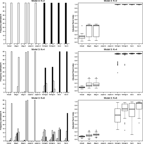
Figure 1: Simulation model 3 ($p=100,n=1000$), number of states and state assignments. Left panels: frequency of estimated number of states; in each case the correct number of states (i.e., number of states in data-generating model) is indicated in black. Right panels: adjusted Rand index with respect to true state assignments. [Legend: Results for Mclust (mclust), MLE with diagonal covariance matrices (diag), MLE (unpen) and Greedy Backward Pruning (bw) are shown. The extensions “.b” and “.m” stand for BIC and MMDL, resp.]

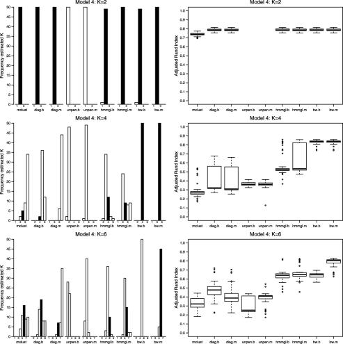
Figure 2: Simulation model 4 ($p=50,n=5000$), number of states and state assignments. Left panels: frequency of estimated number of states (as in Figure 1 correct number of states indicated in black). Right panels: adjusted Rand index with respect to true state assignments. [Legend: Results for Mclust (mclust), MLE with diagonal covariance matrices (diag), MLE (unpen) and Greedy Backward Pruning (bw) are shown. Extensions “.b” and “.m” stand for BIC and MMDL, resp.]

In nearly all settings Diagcov is unable to recover the correct number of states and performs poorly in terms of adjusted Rand index. This is not surprising as Diagcov imposes incorrect model assumptions. Only in model 3 with $K_{\mathrm{true}}=2$, where for both states the data generating covariance matrices are diagonal, does Diagcov perform well. MLE without penalization (Unpen) does well only in the low-dimensional model 1. Both the proposed methods (Hmmgl and Bwprun) greatly outperform the other methods in models 2–4. This supports the notion that regularization can be useful even when sample size $n$ is seemingly large.

HMMGLasso also works well in model 1 with large $n$ and very small $p$, a scenario where no constraints are necessary. This demonstrates that the adaptive strategy and universal regularization can be applied without any hand tuning also in the low-dimensional setting. We also read off from Figures 1–2 (see especially scenarios with $K=6$) the substantial improvement of Greedy Backward Pruning relative to HMMGLasso, despite the fact that the latter carries out essentially a brute-force search over $K$. Also, the use of MMDL further improves performance (it never performs worse than BIC). Especially in tough and very high-dimensional scenarios (models 3 and 4 with $K=6$), MMDL seems to perform better.

Experiment II: Graph structure. In this experiment we focus on recovering state-specific graphical model structure. We consider model 3 with $K_{\mathrm{true}}\in\{2,4,6\}$ and $\alpha\in\{2,6,10\}$. We compare Greedy Backward Pruning, HMMGLasso ($K=K_{\mathrm{true}},\operatorname{Pen}_{\mathrm{parcor}},\lambda_{\mathrm{uni}}$), Kmeans (with number of clusters set to $K=K_{\mathrm{true}}$) followed by estimating cluster-specific inverse covariance matrices using Graphical Lasso, and Graphical Lasso using all samples (no state assignment or clustering). In Figure 3 True Positive Rate (TPR; with respect to edges in the data-generating graph) is plotted against the corresponding False Positive Rate (FPR) for all combinations of $K$ and $\alpha$ and different methods. We note that Greedy Backward Pruning consistently selects the correct number of states in all scenarios except in $(K_{\mathrm{true}},\alpha)=(6,2)$ where it chooses $K$ correctly in 36 out of 50 data sets.

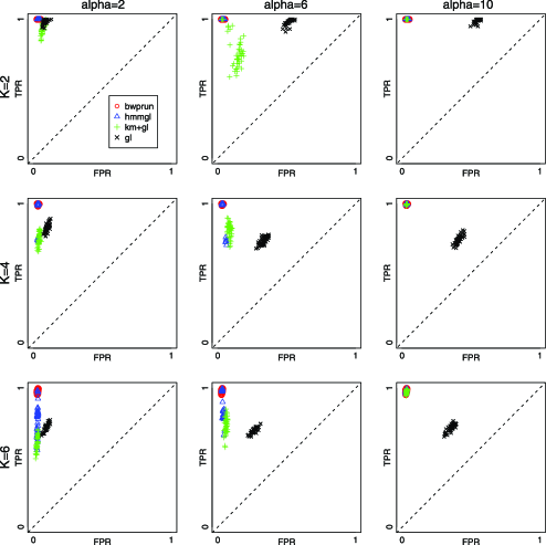
Figure 3: Simulation experiment II, graphical model estimation. Comparing estimated state-specific conditional independence graphs against the data-generating graphs gave true positive and false positive rates with respect to edges in the graphs (TPR and FPR, resp.). We show TPR plotted against FPR with $K\in\{2,4,6\}$, $\alpha\in\{2,6,10\}$ for model 3. [Legend: Results for Greedy Backward Pruning (bwprun), HMMGLasso (hmmgl), Kmeans clustering with cluster-wise Graphical Lasso (km${}+{}$glasso) and Graphical Lasso applied to nonclustered data (glasso) are shown.]

Greedy Backward Pruning performs well in terms of TPR and FPR. It is noteworthy that universal regularization using $\lambda_{\mathrm{uni}}$ gives consistently good results under a range of conditions. We see that HMMGLasso exhibits a smaller true positive rate in the most challenging $K_{\mathrm{true}}=6$ case. For $\alpha=2$ Kmeans in combination with GLasso performs much worse, in particular in terms of TPR. For larger $\alpha$’s (and therefore with increased information about state-assignment in the means) TPR and FPR of Kmeans improves. Finally, GLasso applied to all data without any clustering leads to very poor performance (this is likely a consequence of Simpson’s paradox).

3.2 Application to genomic data

We consider genome-wide binding data for 53 proteins in the Drosophila cell line Kc167 [data from Filion et al. (2010)]. Filion et al. (2010) represents an important step forward in the genome biology of Drosophila, showing how multivariate data can reveal protein-DNA binding patterns that depend on genome region. Here, we use this data set to test our HMM methodology. The data set offers a number of advantages for our purposes. First, the coverage of a relatively large number of proteins ($p=53$) in the full data gives a high-dimensional example from current genome biology. Second, the abundance of data ($n=33\mbox{,}632$ for chromosome 2L and $n=32\mbox{,}791$ for chromsome 2R) allows fully held-out validation on a large test set (we use the latter half of chromsome 2R, giving $n_{\mathrm{test}}=16\mbox{,}396$) as well as exploration of the effect of (training) sample size. Finally, although substantive biological questions are beyond the scope of this paper, several open questions concerning genome organization in Drosophila, including the likely number of genome regions, and the possibility of region-specific protein–protein interplay, help to motivate the methodological questions we address here.

Filion et al. (2010) identified regions of the genome by fitting a HMM (using classical, unpenalized estimation) to reduced-dimension data. Dimensionality reduction was carried out using principal component analysis (PCA) as a preprocessing step, with the HMM fitted to the first three principal components. Such approaches are currently widely used in genome biology. By looking at principal components, Filion et al. (2010) suggested a model with five states (corresponding to different chromatin types). They further noted that these five states are marked by enriched binding of the proteins HP1, PC, H1, BRM and MRG15 and that a 5-state HMM using only the five marker proteins as an input recapitulates $85.5\%$ of the original state classification.

We investigated performance in a held-out predictive sense by training on the first $n_{\mathrm{train}}=500,1000,$ $2000,\ldots,5000$ observations of chromosome 2L and then reporting the test log-likelihood obtained from the second half of chromosome 2R ($n_{\mathrm{test}}=16\mbox{,}396$). As above, we compare HMMGLasso (Hmmgl), Greedy Backward Pruning (Bwprun), unpenalized MLE (Unpen) and MLE with diagonal covariance matrices (Diagcov). Additionally, we include a five-state MLE using only the five marker proteins reported by Filion et al. (2010) (Marker). For Hmmgl, Unpen and Diagcov the number of states is determined by exploring different $K$’s in a forward stepwise manner. We use MMDL and BIC as model selection criteria. All methods are initialized by Kmeans with initial centroids obtained using hierarchical clustering; this renders the overall analysis deterministic by removing variability due to random initialization of Kmeans.

Figure 4 shows the MMDL(BIC)-scores (scaled by $n_{\mathrm{train}}$) and the negative test log-likelihood as a function of $n_{\mathrm{train}}$. Figure 5 depicts the selected number of states for each method and training sample size. Overall, we notice that MMDL (BIC) and test log-likelihood show similar patterns for different methods and different sample sizes. Bwprun and Hmmgl greatly outperform Marker and Diagcov. This provides a topical example where a multivariate view (using all variables and modeling also state-specific covariances) improves out-of-sample predictive performance. The predictive gain of penalization compared to unpenalized MLE for moderate $n/p$-ratios is also noteworthy. As expected, the performance of Unpen in terms of MMDL (BIC) and test log-likelihood approaches the penalized methods with increasing sample size. However, in terms of number of states (Figure 5), the estimates are very different even for large $n_{\mathrm{train}}$, that is, penalization typically leads to more states than unpenalized MLE. This illustrates that the prediction-optimal number of states depends on the estimation procedure employed: regularization allows estimation for a greater number of states. If state-specific estimates have scientific relevance, this property can be important, since, due to Simpson’s paradox, estimates for finer state distinctions (larger $K$) cannot, in general, be recovered from coarser models (smaller $K$). We return to the question of exploration of number of states in the Discussion below.

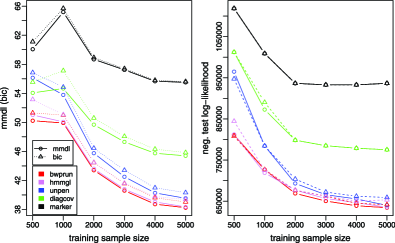
Figure 4: Genomic data, MMDL(BIC) and predictive performance. Models were fitted to protein binding data from Filion et al. (2010) (see text for details) and tested on held-out data from the same study. Left panel: MMDL(BIC)-scores (scaled by $n_{\mathrm{train}}$) for different methods trained on the first $n_{\mathrm{train}}=500,1000,\ldots,5000$ observations of chromosome 2L. Right panel: negative test log-likelihood evaluated on a test set (second half of chromosome 2R; training data is from parts of chromosome 2L). [Legend: Greedy Backward Pruning (Bwprun); HMMGLasso (Hmmgl); Unpenalized MLE (Unpen); MLE with diagonal restricted covariance matrices (Diagcov); Five-state MLE using only marker proteins (Marker).]

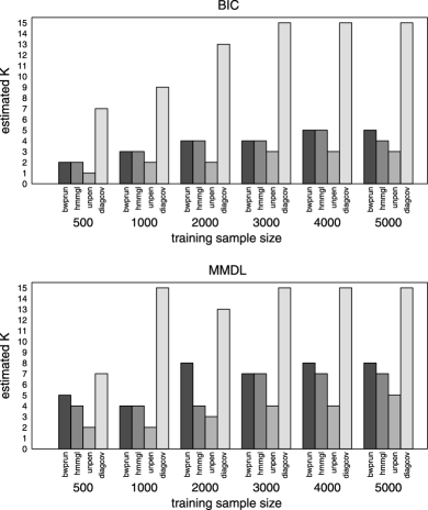
Figure 5: Genomic data, number of states. Number of states selected (at various training sample sizes) by Greedy Backward Pruning (Bwprun), HMMGLasso (Hmmgl), unpenalised MLE (Unpen) and MLE with diagonal restricted covariance matrices (Diagcov). All methods are trained on parts of chromosome 2L and use MMDL or BIC as the model selection criterion. The number of states in Hmmgl, Unpen and Diagcov are determined by a forward stepwise selection.

We note that for each training sample size $n_{\mathrm{train}}$ the results shown in Figures 4–5 reflect performance for a single training sample of the specified length. For completeness, Figure S4 in the supplementary material [Städler and Mukherjee (2013)] shows performance over 9 different training data sets of size $n_{\mathrm{train}}=1000$.

4 Discussion

We considered penalized estimation in multivariate HMMs, including, in particular, the case of high dimensions and state-specific graphical models. As we demonstrated in simulated and real data examples, the methodology we propose substantially improves upon current practice. Our results demonstrate the utility of regularization for HMMs, even when sample sizes are not small.

It is interesting to consider why careful penalization is needed in HMMs (and related latent variable settings like mixture models). In a simple linear model, as in regression, the ratio $n/p$ is a measure to distinguish between a low- and high-dimensional problem. If the ratio $n/p$ is small, classical least-squares estimation leads to poor predictive performance due to a large number of predictors compared to a small sample size. On the other hand, if $n/p$ is large (e.g., $>$20), then, very likely, least-squares regression performs well. In HMMs (and mixtures) the situation is more subtle. It is instructive to consider the ratios $n_{k}/p$ ($n_{k}$ denotes the number of samples belonging to state $k$) as a measure whether an inference problem is high-dimensional or not. If for at least one state this ratio is small, then MLE is likely to overfit and results in a poor generalization error. A fundamental problem that we emphasized throughout the paper is the fact that the ratios $n_{k}/p$ depend on the number of states $K$ and on the state-sizes $n_{k}$, which are themselves usually unknown a priori. So, a seemingly low-dimensional problem with a large sample size and with a moderate number of features can become a high-dimensional task in practice, especially if a large number of states cannot be ruled out a priori. In fact, our simulations illustrate that even when $\min_{k}n_{k}/p$ is relatively large, the MLE can be ill-behaved. For example, in our simulated model 2, with $K=2$, we have $n=2000$ and $n_{k}/p>13$ in each state; nevertheless, the MLE fails completely to recover correct state assignments [see Figure S3, supplementary material, Städler and Mukherjee (2013)].

A straightforward approach to handle inference in high-dimensional HMMs is to fix constraints on the state-specific covariance matrices (e.g., assuming diagonal covariance matrices). However, such an approach leads to poor predictive performance when the assumption is invalid and precludes discovery of state-specific covariance structure. As in the genome biology example we considered, such structure may itself be of scientific interest. We note also that the hidden nature of the states makes it difficult to test any such model assumption. In fact, if the covariance matrices of an HMM with a specific number of states satisfy some constraints, then these constraints do not necessarily hold for an HMM with smaller or larger number of states (Simpson’s paradox).

Estimation of the number of states in a HMM (or mixture model) remains challenging. The backward pruning approach we proposed gives an efficient way to estimate parameters for a sequence of candidate number of states $K$. If desired, a single “optimal” number of states can then be selected using model selection criteria, as we demonstrated in the examples above. Several recent efforts in genome biology have sought to use statistical criteria to elucidate the number of states in the genome [Filion et al. (2010), Ernst and Kellis (2010)] and the methodology we propose can help to further explore this question in a truly multivariate manner. However, it is important to emphasize the limitations of model selection approaches in scientific settings of this kind. Under model misspecification, in general there is no guarantee that the correct number of states will be selected. To illustrate this effect empirically, we simulated data under model 3, but with contamination by samples drawn from a multivariate t distribution [Figure S5, supplementary material, Städler and Mukherjee (2013)]. We find that although estimation of the number of states holds up well for lighter tailed contamination, for heavier tails it is demonstrably inaccurate. Such behavior is unsurprising, even in the large sample setting, since under model misspecification we would then expect to recover the model closest in Kullback–Leibler sense to the data-generating model, which may not be the model with the scientifically correct number of states. These observations underline the need for care in scientific applications where the number of states may have a physical or biological interpretation and where some degree of model misspecification is likely unavoidable [in the related setting of mixture modeling, see, e.g., the discussion in Hennig and Liao (2013)].

In light of the foregoing observations concerning model misspecification, it is interesting to consider the interplay between model selection and regularization. For a given estimator, the optimal number of states is well defined in a predictive sense as the value that minimizes risk. From this point of view it is easy to understand why the prediction-optimal number of states may be higher under regularization or when more training data are available (see Figure 5). For these reasons, when scientific understanding rather than prediction alone is one of the goals of analysis, it is not clear whether it is useful to think in terms of a “correct” number of states. Rather, it may be useful to think of estimates $\{\Theta_{K}\}$ (obtained, e.g., via backward pruning) as collectively providing a resource for exploration of a system of interest.

In the context of mixtures, there is a growing literature on penalized likelihood methods which address the high-dimensional context to some extent [Khalili and Chen (2007), Städler, Bühlmann and van de Geer (2010), Pan and Shen (2007), Hill and Mukherjee (2013)]. However, none of these methods addresses the need to ensure penalties are able to handle state-specific scaling (that cannot be dealt with by preprocessing) and size (i.e., unknown at the outset). The selection of the number of mixture components also remains an open issue in this literature. Our approach handles these issues that arise due to the hidden nature of the states and could be straightforwardly applied in the mixture model setting. Further generalization to other latent variable models may also be possible.

In the genome biology example we considered, penalization led to gains in predictive ability relative to the MLE and to reduced dimension approaches that have been used in the literature. This suggests that despite redundancy in biological signals, a multivariate view can enhance predictive ability. Further, we were able to learn richer models than are possible using currently available methods, including estimates of state-specific graphical model structure. The latter may shed light on protein–protein interplay that is specific to genomic region; such interplay has not been investigated to date and is one focus of our ongoing efforts in this application area. We used data from Filion et al. (2010); we note that the main substantive conclusions drawn in that paper are broadly supported by our analyses and the richer set of states uncovered by our approach are related to the states they report. Genomic data sets are becoming increasingly high-dimensional and we anticipate that the methodology presented here will be useful to researchers in that field. Beyond biology, potential applications for high-dimensional HMMs are numerous, including in signal processing and finance.

We showed that the approaches we put forward for HMMs, including universal regularization and Greedy Backward Pruning, work well in empirical examples. However, there remains a need for theoretical investigation of these ideas. Our penalty in combination with $\lambda_{\mathrm{uni}}$ was inspired by making connections to results obtained for the well-studied Lasso case. A challenge for future theoretical work is to provide insight into optimality of these and related approaches and to establish global convergence properties of penalized estimation in latent variable settings.

References

- Barron et al. (2008) {bbook}[auto:STB—2013/06/05—13:45:01] \bauthor\bsnmBarron, \bfnmA.\binitsA., \bauthor\bsnmHuang, \bfnmC.\binitsC., \bauthor\bsnmLi, \bfnmJ. Q.\binitsJ. Q. and \bauthor\bsnmLuo, \bfnmX.\binitsX. (\byear2008). \btitleMDL Principle, Penalized Likelihood, and Statistical Risk. MIT Press Books. \bpublisherTampere Univ. Press, \blocationTampere, Finland.\bptokimsref\endbibitem
- Bicego, Murino and Figueiredo (2003) {barticle}[auto:STB—2013/06/05—13:45:01] \bauthor\bsnmBicego, \bfnmM.\binitsM., \bauthor\bsnmMurino, \bfnmV.\binitsV. and \bauthor\bsnmFigueiredo, \bfnmM. A. T.\binitsM. A. T. (\byear2003). \btitleA sequential pruning strategy for the selection of the number of states in hidden Markov models. \bjournalPattern Recognition Letters \bvolume24 \bpages1395–1407. \bptokimsref \endbibitem
- Bühlmann and van de Geer (2011) {bbook}[mr] \bauthor\bsnmBühlmann, \bfnmPeter\binitsP. and \bauthor\bparticlevan de \bsnmGeer, \bfnmSara\binitsS. (\byear2011). \btitleStatistics for High-Dimensional Data: Methods, Theory and Applications. \bpublisherSpringer, \blocationHeidelberg. \biddoi=10.1007/978-3-642-20192-9, mr=2807761 \bptokimsref \endbibitem
- Donoho and Johnstone (1994) {barticle}[mr] \bauthor\bsnmDonoho, \bfnmDavid L.\binitsD. L. and \bauthor\bsnmJohnstone, \bfnmIain M.\binitsI. M. (\byear1994). \btitleIdeal spatial adaptation by wavelet shrinkage. \bjournalBiometrika \bvolume81 \bpages425–455. \biddoi=10.1093/biomet/81.3.425, issn=0006-3444, mr=1311089 \bptokimsref \endbibitem
- Durbin et al. (1998) {bbook}[auto:STB—2013/06/05—13:45:01] \bauthor\bsnmDurbin, \bfnmR.\binitsR., \bauthor\bsnmEddy, \bfnmS. R.\binitsS. R., \bauthor\bsnmKrogh, \bfnmA.\binitsA. and \bauthor\bsnmMitchison, \bfnmG. J.\binitsG. J. (\byear1998). \btitleBiological Sequence Analysis: Probabilistic Models of Proteins and Nucleic Acids. \bpublisherCambridge Univ. Press, \blocationCambridge. \bptokimsref \endbibitem
- ENCODE Project Consortium (2012) {bmisc}[pbm] \borganizationENCODE Project Consortium (\byear2012). \bhowpublishedAn integrated encyclopedia of DNA elements in the human genome. Nature 489 57–74. \bptokimsref \endbibitem
- Ernst and Kellis (2010) {barticle}[pbm] \bauthor\bsnmErnst, \bfnmJason\binitsJ. and \bauthor\bsnmKellis, \bfnmManolis\binitsM. (\byear2010). \btitleDiscovery and characterization of chromatin states for systematic annotation of the human genome. \bjournalNat. Biotechnol. \bvolume28 \bpages817–825. \biddoi=10.1038/nbt.1662, issn=1546-1696, mid=NIHMS214961, pii=nbt.1662, pmcid=2919626, pmid=20657582 \bptokimsref \endbibitem
- Figueiredo and Jain (2000) {barticle}[auto:STB—2013/06/05—13:45:01] \bauthor\bsnmFigueiredo, \bfnmM. A. T.\binitsM. A. T. and \bauthor\bsnmJain, \bfnmA. K.\binitsA. K. (\byear2000). \btitleUnsupervised learning of finite mixture models. \bjournalIEEE Transactions on Pattern Analysis and Machine Intelligence \bvolume24 \bpages381–396. \bptokimsref \endbibitem
- Figueiredo, Leitão and Jain (1999) {bincollection}[auto:STB—2013/06/05—13:45:01] \bauthor\bsnmFigueiredo, \bfnmM. A. T.\binitsM. A. T., \bauthor\bsnmLeitão, \bfnmJ. M. N.\binitsJ. M. N. and \bauthor\bsnmJain, \bfnmA. K.\binitsA. K. (\byear1999). \btitleOn fitting mixture models. In \bbooktitleProceedings of the Second International Workshop on Energy Minimization Methods in Computer Vision and Pattern Recognition, EMMCVPR’99 \bpages54–69. \bpublisherSpringer, \baddressBerlin. \bptokimsref \endbibitem
- Filion et al. (2010) {barticle}[pbm] \bauthor\bsnmFilion, \bfnmGuillaume J.\binitsG. J., \bauthor\bparticlevan \bsnmBemmel, \bfnmJoke G.\binitsJ. G., \bauthor\bsnmBraunschweig, \bfnmUlrich\binitsU., \bauthor\bsnmTalhout, \bfnmWendy\binitsW., \bauthor\bsnmKind, \bfnmJop\binitsJ., \bauthor\bsnmWard, \bfnmLucas D.\binitsL. D., \bauthor\bsnmBrugman, \bfnmWim\binitsW., \bauthor\bparticlede \bsnmCastro, \bfnmInês J.\binitsI. J., \bauthor\bsnmKerkhoven, \bfnmRon M.\binitsR. M., \bauthor\bsnmBussemaker, \bfnmHarmen J.\binitsH. J. and \bauthor\bparticlevan \bsnmSteensel, \bfnmBas\binitsB. (\byear2010). \btitleSystematic protein location mapping reveals five principal chromatin types in Drosophila cells. \bjournalCell \bvolume143 \bpages212–224. \biddoi=10.1016/j.cell.2010.09.009, issn=1097-4172, mid=NIHMS237730, pii=S0092-8674(10)01057-3, pmcid=3119929, pmid=20888037 \bptokimsref \endbibitem
- Fraley and Raftery (2002) {barticle}[mr] \bauthor\bsnmFraley, \bfnmChris\binitsC. and \bauthor\bsnmRaftery, \bfnmAdrian E.\binitsA. E. (\byear2002). \btitleModel-based clustering, discriminant analysis, and density estimation. \bjournalJ. Amer. Statist. Assoc. \bvolume97 \bpages611–631. \biddoi=10.1198/016214502760047131, issn=0162-1459, mr=1951635 \bptokimsref \endbibitem
- Fraley and Raftery (2006) {bmisc}[auto:STB—2013/06/05—13:45:01] \bauthor\bsnmFraley, \bfnmC.\binitsC. and \bauthor\bsnmRaftery, \bfnmA. E.\binitsA. E. (\byear2006). \bhowpublishedMCLUST version 3 for R: Normal mixture modeling and model-based clustering. Technical Report 504, Dept. Statistics, Univ. Washington, Seattle, WA. \bptokimsref \endbibitem
- Friedman, Hastie and Tibshirani (2008) {barticle}[pbm] \bauthor\bsnmFriedman, \bfnmJerome\binitsJ., \bauthor\bsnmHastie, \bfnmTrevor\binitsT. and \bauthor\bsnmTibshirani, \bfnmRobert\binitsR. (\byear2008). \btitleSparse inverse covariance estimation with the graphical lasso. \bjournalBiostatistics \bvolume9 \bpages432–441. \biddoi=10.1093/biostatistics/kxm045, issn=1468-4357, mid=NIHMS248717, pii=kxm045, pmcid=3019769, pmid=18079126 \bptokimsref \endbibitem
- Grünwald (2007) {bbook}[auto:STB—2013/06/05—13:45:01] \bauthor\bsnmGrünwald, \bfnmP. D.\binitsP. D. (\byear2007). \btitleThe Minimum Description Length Principle. \bpublisherMIT Press, \blocationCambridge, MA. \bptokimsref \endbibitem
- Hennig and Liao (2013) {barticle}[auto:STB—2013/06/05—13:45:01] \bauthor\bsnmHennig, \bfnmC.\binitsC. and \bauthor\bsnmLiao, \bfnmT. F.\binitsT. F. (\byear2013). \btitleHow to find an appropriate clustering for mixed type variables with application to socio-economic stratification. \bjournalJ. R. Stat. Soc. Ser. C. Appl. Stat. \bvolume62 \bpages309–369. \bptokimsref \endbibitem
- Hill and Mukherjee (2013) {bmisc}[auto:STB—2013/06/05—13:45:01] \bauthor\bsnmHill, \bfnmS. M.\binitsS. M. and \bauthor\bsnmMukherjee, \bfnmS.\binitsS. (\byear2013). \bhowpublishedNetwork-based clustering with mixtures of L1-penalized Gaussian graphical models: An empirical investigation. Available at \arxivurlarXiv:1301.2194. \bptokimsref \endbibitem
- Khalili and Chen (2007) {barticle}[mr] \bauthor\bsnmKhalili, \bfnmAbbas\binitsA. and \bauthor\bsnmChen, \bfnmJiahua\binitsJ. (\byear2007). \btitleVariable selection in finite mixture of regression models. \bjournalJ. Amer. Statist. Assoc. \bvolume102 \bpages1025–1038. \biddoi=10.1198/016214507000000590, issn=0162-1459, mr=2411662 \bptokimsref \endbibitem
- Krogh, Mian and Haussler (1994) {barticle}[auto:STB—2013/06/05—13:45:01] \bauthor\bsnmKrogh, \bfnmA.\binitsA., \bauthor\bsnmMian, \bfnmI. S.\binitsI. S. and \bauthor\bsnmHaussler, \bfnmD.\binitsD. (\byear1994). \btitleA hidden Markov model that finds genes in E. coli DNA. \bjournalNucleic Acids Res. \bvolume22 \bpages4768–4778. \bptokimsref \endbibitem
- Meinshausen and Bühlmann (2006) {barticle}[mr] \bauthor\bsnmMeinshausen, \bfnmNicolai\binitsN. and \bauthor\bsnmBühlmann, \bfnmPeter\binitsP. (\byear2006). \btitleHigh-dimensional graphs and variable selection with the lasso. \bjournalAnn. Statist. \bvolume34 \bpages1436–1462. \biddoi=10.1214/009053606000000281, issn=0090-5364, mr=2278363 \bptokimsref \endbibitem
- Pan and Shen (2007) {barticle}[auto:STB—2013/06/05—13:45:01] \bauthor\bsnmPan, \bfnmW.\binitsW. and \bauthor\bsnmShen, \bfnmX.\binitsX. (\byear2007). \btitlePenalized model-based clustering with application to variable selection. \bjournalJ. Mach. Learn. Res. \bvolume8 \bpages1145–1164. \bptokimsref \endbibitem
- Park (2009) {barticle}[auto:STB—2013/06/05—13:45:01] \bauthor\bsnmPark, \bfnmP.\binitsP. (\byear2009). \btitleChIP–seq: Advantages and challenges of a maturing technology. \bjournalNature Reviews Genetics \bvolume10 \bpages669–680. \bptokimsref \endbibitem
- Rothman et al. (2008) {barticle}[mr] \bauthor\bsnmRothman, \bfnmAdam J.\binitsA. J., \bauthor\bsnmBickel, \bfnmPeter J.\binitsP. J., \bauthor\bsnmLevina, \bfnmElizaveta\binitsE. and \bauthor\bsnmZhu, \bfnmJi\binitsJ. (\byear2008). \btitleSparse permutation invariant covariance estimation. \bjournalElectron. J. Stat. \bvolume2 \bpages494–515. \biddoi=10.1214/08-EJS176, issn=1935-7524, mr=2417391 \bptokimsref \endbibitem
- Städler, Bühlmann and van de Geer (2010) {barticle}[mr] \bauthor\bsnmStädler, \bfnmNicolas\binitsN., \bauthor\bsnmBühlmann, \bfnmPeter\binitsP. and \bauthor\bparticlevan de \bsnmGeer, \bfnmSara\binitsS. (\byear2010). \btitle-penalization for mixture regression models. \bjournalTEST \bvolume19 \bpages209–256. \biddoi=10.1007/s11749-010-0197-z, issn=1133-0686, mr=2677722 \bptnotecheck related\bptokimsref \endbibitem
- Städler and Mukherjee (2013) {bmisc}[auto:STB—2013/06/05—13:45:01] \bauthor\bsnmStädler, \bfnmN.\binitsN. and \bauthor\bsnmMukherjee, \bfnmS.\binitsS. (\byear2013). \bhowpublishedSupplement to “Penalized estimation in high-dimensional hidden Markov models with state-specific graphical models.” DOI:\doiurl10.1214/13-AOAS662SUPP. \bptokimsref \endbibitem
- Sun and Zhang (2012) {barticle}[mr] \bauthor\bsnmSun, \bfnmTingni\binitsT. and \bauthor\bsnmZhang, \bfnmCun-Hui\binitsC.-H. (\byear2012). \btitleScaled sparse linear regression. \bjournalBiometrika \bvolume99 \bpages879–898. \biddoi=10.1093/biomet/ass043, issn=0006-3444, mr=2999166 \bptnotecheck year\bptokimsref \endbibitem
- Tibshirani (1996) {barticle}[mr] \bauthor\bsnmTibshirani, \bfnmRobert\binitsR. (\byear1996). \btitleRegression shrinkage and selection via the lasso. \bjournalJ. R. Stat. Soc. Ser. B Stat. Methodol. \bvolume58 \bpages267–288. \bidissn=0035-9246, mr=1379242 \bptokimsref \endbibitem
- van Steensel and Henikoff (2000) {barticle}[pbm] \bauthor\bparticlevan \bsnmSteensel, \bfnmB.\binitsB. and \bauthor\bsnmHenikoff, \bfnmS.\binitsS. (\byear2000). \btitleIdentification of in vivo DNA targets of chromatin proteins using tethered dam methyltransferase. \bjournalNat. Biotechnol. \bvolume18 \bpages424–428. \biddoi=10.1038/74487, issn=1087-0156, pmid=10748524 \bptokimsref \endbibitem
- Yuan and Lin (2007) {barticle}[mr] \bauthor\bsnmYuan, \bfnmMing\binitsM. and \bauthor\bsnmLin, \bfnmYi\binitsY. (\byear2007). \btitleModel selection and estimation in the Gaussian graphical model. \bjournalBiometrika \bvolume94 \bpages19–35. \biddoi=10.1093/biomet/asm018, issn=0006-3444, mr=2367824 \bptokimsref \endbibitem
- Zhang (2010) {barticle}[mr] \bauthor\bsnmZhang, \bfnmCun-Hui\binitsC.-H. (\byear2010). \btitleNearly unbiased variable selection under minimax concave penalty. \bjournalAnn. Statist. \bvolume38 \bpages894–942. \biddoi=10.1214/09-AOS729, issn=0090-5364, mr=2604701 \bptokimsref \endbibitem