New scaling for the alpha effect in slowly rotating turbulence

Abstract

Using simulations of slowly rotating stratified turbulence, we show that the $\alpha$ effect responsible for the generation of astrophysical magnetic fields is proportional to the logarithmic gradient of kinetic energy density rather than that of momentum, as was previously thought. This result is in agreement with a new analytic theory developed in this paper for large Reynolds numbers. Thus, the contribution of density stratification is less important than that of turbulent velocity. The $\alpha$ effect and other turbulent transport coefficients are determined by means of the test-field method. In addition to forced turbulence, we also investigate supernova-driven turbulence and stellar convection. In some cases (intermediate rotation rate for forced turbulence, convection with intermediate temperature stratification, and supernova-driven turbulence) we find that the contribution of density stratification might be even less important than suggested by the analytic theory.

1. Introduction

Turbulent dynamos occur in many astrophysical situations. They tend to develop large-scale magnetic structures in space and time that are generally understood in terms of mean-field dynamo theory (e.g. Moffatt, 1978; Parker, 1979; Krause & Rädler, 1980; Zeldovich et al., 1983; Ruzmaikin et al., 1988; Rüdiger & Hollerbach, 2004; Brandenburg & Subramanian, 2005). Central to this theory is the $\alpha$ effect, which denotes a contribution to the mean electromotive force that is given by a pseudo-scalar $\alpha$ multiplying the mean magnetic field. Such a pseudo-scalar can be the result of rotation, $\bm{\Omega}$, combined with stratification of density and/or turbulence intensity, $\mbox{\boldmath$\nabla$}{}\overline{\rho}$ and/or $\mbox{\boldmath$\nabla$}{}u_{\rm rms}$, respectively. Here, $\overline{\rho}$ is the mean gas density and $u_{\rm rms}=(\overline{{\bm{u}}^{2}})^{1/2}$ is the rms value of the turbulent velocity, ${\bm{u}}$.

There have been a number of analytic studies quantifying the effects of rotating stratified turbulence on the mean electromotive force (Krause & Rädler, 1980; Kichatinov, 1991; Rüdiger & Kichatinov, 1993; Kitchatinov et al., 1994; Rädler et al., 2003; Kleeorin & Rogachevskii, 2003). In particular, it was found, using the quasi-linear approach (or second-order correlation approximation), that the diagonal components of the $\alpha$ tensor for slow rotation rate (or small Coriolis numbers) are given by (Steenbeck et al., 1966; Krause & Rädler, 1980)

$$\alpha\approx-\ell_{\alpha}^{2}\bm{\Omega}\cdot\mbox{\boldmath$\nabla$}{}\ln(\overline{\rho}\,u_{\rm rms}),$$ (1)

where $\ell_{\alpha}=\tau_{0}u_{\rm rms}$ is a relevant length scale and $\tau_{0}$ is the characteristic turbulent time related to the turnover time.

In the solar convective zone the mean fluid density $\overline{\rho}$ changes by seven orders of magnitudes, while the turbulent kinetic energy ($\approx\overline{\rho}u_{\rm rms}^{2}/2$) changes by only three orders of magnitudes and, according to stellar mixing length theory (Vitense, 1953), $\overline{\rho}\,u_{\rm rms}^{3}$ would be approximately constant in the solar convective zone. Here the fluid density $\rho$ is the sum of the mean and fluctuating density. This issue has become timely, because there is a new numerical technique that allows the different proposals to be examined with sufficient accuracy. The so-called test-field method (Schrinner et al., 2005, 2007) allows one to determine all the relevant turbulent transport coefficients in the expression for the mean electromotive force without the restrictions of some of the analytic approaches such as the quasi-linear approach, the path-integral approach or the $\tau$ approach. With the test-field method one solves sets of equations for the small-scale fields resulting from different prescribed mean fields — the test fields. These equations resemble the usual induction equation, except that they contain an additional inhomogeneous term.

This method is quite powerful because it has been shown to be rather accurate and it gives not only the tensor coefficients of $\alpha$ effect and turbulent diffusivity, but it also allows the scale-dependence to be determined, which means that these coefficients are actually integral kernels that allow the effects of neighboring points in space and time to be taken into account. For details regarding scale separation, see Brandenburg et al. (2008) and Hubbard & Brandenburg (2009). We apply this method to numerical simulations of forced turbulence in a stably stratified layer in the presence of rotation and a prescribed vertical dependence of the turbulence intensity. We also use test-field method in simulations of turbulent convection and supernova-driven turbulence of the interstellar medium (ISM).

The goal of the present paper is to determine the correct scaling of the $\alpha$ effect with mean density and rms velocity for slow rotation, i.e., when the Coriolis number ${\rm Co}\equiv 2\Omega\tau_{0}$ is much less than unity, and large Reynolds numbers. In addition to the parameter $\ell_{\alpha}$, we determine the exponent $\sigma$ in the diagonal components of the $\alpha$ tensor,

$$\alpha=-\ell_{\alpha}^{2}\bm{\Omega}\cdot\mbox{\boldmath$\nabla$}{}\ln(\overline{\rho}^{\sigma}u_{\rm rms}).$$ (2)

Such an ansatz was also made by Rüdiger & Kichatinov (1993), who found that in the high conductivity limit, $\sigma=3/2$ for slow rotation and $\sigma=1$ for rapid rotation. However, as we will show in this paper, both numerically (for forced turbulence and for turbulent convection with stronger temperature stratification and overshoot layer) as well as analytically, our results for slow rotation and large fluid and magnetic Reynolds numbers are consistent with $\sigma=1/2$. In some simulations we also found $\sigma=1/3$.

2. Theoretical predictions

We consider the kinematic problem, i.e., we neglect the feedback of the magnetic field on the turbulent fluid flow. We use a mean field approach whereby velocity, pressure and magnetic field are separated into mean and fluctuating parts. Unlike in earlier derivations, and to maintain maximum generality, we allow the characteristic scales of the mean fluid density, $\overline{\rho}$, the turbulent kinetic energy, $\overline{\rho}u_{\rm rms}^{2}/2$, and the variations of $\overline{\rho}\,u_{\rm rms}^{3}$ to be different. We also assume vanishing mean motion. The strategy of our analytic derivation is to determine the $\Omega$ dependencies of the second moments for the velocity $\overline{u_{i}(t,{\bm{x}})\,u_{j}(t,{\bm{x}})}$ and for the cross-helicity tensor $\overline{b_{i}(t,{\bm{x}})\,u_{j}(t,{\bm{x}})}$, where ${\bm{b}}$ are fluctuations of magnetic field produced by tangling of the large-scale field. To this end we use the equations for fluctuations of velocity and magnetic field in rotating turbulence, which are obtained by subtracting equations for the mean fields from the corresponding equations for the actual (mean plus fluctuating) fields.

2.1. Governing equations

The equations for the fluctuations of velocity and magnetic fields are given by

$${\partial{\bm{u}}\over\partial t} = -c_{\rm s}^{2}{\mbox{\boldmath$\nabla$}\rho^{\prime}\over\overline{\rho}}+2{\bm{u}}\times{\bm{\Omega}}+\hat{\cal N}({\bm{u}}),$$ (3)

$${\partial{\bm{b}}\over\partial t} = (\overline{\mbox{\boldmath$B$}}{}\cdot\mbox{\boldmath$\nabla$}){\bm{u}}-({\bm{u}}\cdot\mbox{\boldmath$\nabla$})\overline{\mbox{\boldmath$B$}}{}-\overline{\mbox{\boldmath$B$}}{}(\mbox{\boldmath$\nabla$}\cdot{\bm{u}})+\hat{\cal N}({\bm{b}}),$$ (4)

$${\partial\rho^{\prime}\over\partial t} = -\mbox{\boldmath$\nabla$}{}\cdot(\overline{\rho}{\bm{u}})-\mbox{\boldmath$\nabla$}{}\cdot(\rho^{\prime}{\bm{u}}),$$ (5)

where Equation (3) is written in a reference frame rotating with constant angular velocity ${\bm{\Omega}}$, and $\rho^{\prime}=\rho-\overline{\rho}$ is the fluctuating density. We consider an isothermal equation of state, $p=c_{\rm s}^{2}\rho$, so that the density scale height is then constant. Here, $c_{\rm s}={\rm const}{}$ is the sound speed, $\overline{\mbox{\boldmath$B$}}{}$ is the mean magnetic field, $p$ and $\rho$ are the full (mean plus fluctuating) fluid pressure and density, respectively. The terms $\hat{\cal N}({\bm{u}})$ and $\hat{\cal N}({\bm{b}})$, which include nonlinear and molecular viscous and dissipative terms, are given by

$$\hat{\cal N}({\bm{u}}) = \overline{({\bm{u}}\cdot\mbox{\boldmath$\nabla$}){\bm{u}}}-({\bm{u}}\cdot\mbox{\boldmath$\nabla$}){\bm{u}}+{\bm{f}}_{\nu}({\bm{u}}),$$ (6)

$$\hat{\cal N}({\bm{b}}) = \mbox{\boldmath$\nabla$}\times\left({\bm{u}}\times{\bm{b}}-\overline{{\bm{u}}\times{\bm{b}}}-\eta\mbox{\boldmath$\nabla$}\times{\bm{b}}\right),$$ (7)

where $\overline{\rho}{\bm{f}}_{\nu}({\bm{u}})$ is the molecular viscous force and $\eta$ is the magnetic diffusion due to the electrical conductivity of the fluid.

2.2. The derivation procedure

To study rotating turbulence we perform derivations which include the following steps:

(i) use new variables $({\bm{V}},\,\overline{\mbox{\boldmath$H$}}{})$ and perform derivations which include the fluctuations of rescaled velocity ${\bm{V}}=\overline{\rho}^{\sigma}\,{\bm{u}}$ and the mean magnetic field $\overline{\mbox{\boldmath$H$}}{}=\overline{\mbox{\boldmath$B$}}{}/\overline{\rho}^{\sigma}$;

(ii) derive equations for the second moments of the velocity fluctuations $\overline{V_{i}\,V_{j}}$ and the cross-helicity tensor $\overline{b_{i}\,V_{j}}$ in ${\bm{k}}$ space;

(iii) apply the spectral closure, e.g., the spectral $\tau$ approximation (Pouquet et al., 1976; Kleeorin et al., 1990) for large fluid and magnetic Reynolds numbers and solve the derived second-moment equations in ${\bm{k}}$ space;

(iv) return to physical space to obtain formulae for the Reynolds stress and the cross-helicity tensor as functions of $\Omega$. The resulting equations allow us then to obtain the $\Omega$ dependence of the $\alpha$ effect. In these derivations we only take into account effects that are linear in both ${\bm{\lambda}}$ and ${\bm{\Omega}}$, where $\mbox{\boldmath$\lambda$}=-\mbox{\boldmath$\nabla$}\ln\overline{\rho}$.

To exclude the pressure term from Equation (3) we take twice the curl of the momentum equation written in the new variables. The equations which follow from Equations (3) and (4), are given by:

$${\partial\over\partial t}\left[\mbox{\boldmath$\nabla$}^{(\lambda)}\left(\mbox{\boldmath$\lambda$}\cdot{\bm{V}}\right)-\left(\mbox{\boldmath$\nabla$}^{(\lambda)}\right)^{2}{\bm{V}}\right]=2\left({\bm{\Omega}}\cdot\mbox{\boldmath$\nabla$}^{(\lambda)}\right)$$

$$\quad\quad\times\left(\mbox{\boldmath$\nabla$}^{(\lambda)}\times{\bm{V}}\right)+2\left({\bm{\Omega}}\times\mbox{\boldmath$\nabla$}^{(\lambda)}\right)\left(\mbox{\boldmath$\nabla$}^{(\lambda)}\cdot{\bm{V}}\right),$$

$$\quad\quad+\hat{\cal N}({\bm{V}})$$ (8)

$${\partial{\bm{b}}\over\partial t}=\left(\overline{\mbox{\boldmath$H$}}{}\cdot\mbox{\boldmath$\nabla$}^{(\lambda)}\right){\bm{V}}-\left({\bm{V}}\cdot\mbox{\boldmath$\nabla$}^{(\lambda)}\right)\overline{\mbox{\boldmath$H$}}{}$$

$$\quad\quad+(2\sigma-1)\left(\mbox{\boldmath$\nabla$}^{(\lambda)}\cdot{\bm{V}}\right)\overline{\mbox{\boldmath$H$}}{}+\hat{\cal N}({\bm{b}}),$$ (9)

where $\mbox{\boldmath$\nabla$}^{(\lambda)}=\mbox{\boldmath$\nabla$}+\sigma\mbox{\boldmath$\lambda$}$. Furthermore, $\hat{\cal N}({\bm{V}})=\mbox{\boldmath$\nabla$}{\bm{\times}}\left(\mbox{\boldmath$\nabla$}{\bm{\times}}\hat{\cal N}({\bm{u}})\right)$ is the nonlinear term. We consider two cases: (i) low Mach numbers, where the fluid velocity fluctuations ${\bm{V}}$ satisfy the equation $\mbox{\boldmath$\nabla$}\cdot{\bm{V}}=(1-\sigma)({\bm{V}}\cdot\mbox{\boldmath$\lambda$})$ in the anelastic approximation, and (ii) fluid flow with arbitrary Mach numbers, where velocity fluctuations satisfy continuity equation Equation (5). To derive Equation (8) we use the identities given in Appendix A.

2.3. Two-scale approach

We apply the standard two-scale approach with slow and fast variables, e.g., a correlation function,

$$\overline{V_{i}({\bm{x}})V_{j}({\bm{y}})}=\int\int\,d{\bm{k}}_{1}\,d{\bm{k}}_{2}\,\overline{V_{i}({\bm{k}}_{1})V_{j}({\bm{k}}_{2})}\exp\{i({\bm{k}}_{1}{\bm{\cdot}}{\bm{x}}$$

$$\quad+{\bm{k}}_{2}{\bm{\cdot}}{\bm{y}})\}=\int\int\,d{\bm{k}}\,d{\bm{K}}\,f_{ij}({\bm{k},K})\exp(i{\bm{k}}{\bm{\cdot}}{\bm{r}}+i{\bm{K}}{\bm{\cdot}}{\bm{R}})$$

$$\quad=\int\,d{\bm{k}}\,f_{ij}({\bm{k},R})\exp(i{\bm{k}}{\bm{\cdot}}{\bm{r}}),$$

(see, e.g., Roberts & Soward, 1975). Hereafter we omit the argument $t$ in the correlation functions, $f_{ij}({\bm{k},R})=\hat{L}(V_{i};V_{j})$, where

$$\hat{L}(a;c)=\int\overline{a({\bm{k}}+{\textstyle{1\over 2}}{\bm{K}})c(-{\bm{k}}+{\textstyle{1\over 2}}{\bm{K}})}\exp{(i{\bm{K}}{\bm{\cdot}}{\bm{R}})}\,d{\bm{K}},$$

and we have introduced the new variables ${\bm{R}}={\textstyle{1\over 2}}({\bm{x}}+{\bm{y}})$, ${\bm{r}}={\bm{x}}-{\bm{y}}$, $\,{\bm{K}}={\bm{k}}_{1}+{\bm{k}}_{2}$, ${\bm{k}}={\textstyle{1\over 2}}({\bm{k}}_{1}-{\bm{k}}_{2})$. The variables ${\bm{R}}$ and ${\bm{K}}$ correspond to large scales, while ${\bm{r}}$ and ${\bm{k}}$ correspond to small scales. This implies that we assume that there exists a separation of scales, i.e., the maximum scale of turbulent motions $\ell_{0}$ is much smaller than the characteristic scale $L_{B}$ of inhomogeneity of the mean magnetic field.

2.4. Equations for the second moments

Using Equations (8) and (9) written in ${\bm{k}}$ space, we derive equations for the following correlation functions: $f_{ij}({\bm{k}},{\bm{K}})=\overline{V_{i}(t,{\bm{k}}_{1})V_{j}(t,{\bm{k}}_{2})}$ and $g_{ij}({\bm{k}},{\bm{K}})=\overline{b_{i}(t,{\bm{k}}_{1})V_{j}(t,{\bm{k}}_{2})}$. The equations for these correlation functions are given by

$${\partial f_{ij}\over\partial t} = -2\Omega_{l}\Big{[}\varepsilon_{ipq}\Lambda_{pl}^{(1)}f_{qj}+\varepsilon_{jpq}\Lambda_{pl}^{(2)}f_{iq}+{i\lambda_{n}\over k^{2}}\Big{(}\varepsilon_{jlq}k_{q}f_{in}$$ (10)

$$-\varepsilon_{ilq}k_{q}f_{nj}+\varepsilon_{npq}k_{pl}\big{(}k_{j}f_{iq}-k_{i}f_{qj}\big{)}\Big{)}\Big{]}$$

$$+I^{f}_{ij}+\hat{\cal N}f_{ij},$$

$${\partial g_{ij}\over\partial t} = -2\Omega_{l}\Big{[}\varepsilon_{jpq}\Lambda_{pl}^{(2)}g_{iq}+{i\lambda_{n}\over k^{2}}\Big{(}\varepsilon_{jlq}k_{q}g_{in}$$ (11)

$$+k\varepsilon_{npq}k_{plj}g_{iq}\Big{)}\Big{]}+i\left({\bm{\Lambda}}^{(1)}\cdot\overline{\mbox{\boldmath$H$}}{}\right)f_{ij}-\overline{H}_{i}\lambda_{n}f_{nj}$$

$$+I^{g}_{ij}+\hat{\cal N}g_{ij},$$

where $k_{ij}=k_{i}k_{j}/k^{2}$, ${\bm{\Lambda}}^{(1)}={\bm{k}}_{1}-i\sigma{\bm{\lambda}}$, and similarly for ${\bm{\Lambda}}^{(2)}$, $\Lambda_{mn}^{(1)}=\Lambda_{m}^{(1)}\Lambda_{n}^{(1)}/({\bm{\Lambda}}^{(1)})^{2}$, and similarly for $\Lambda_{mn}^{(2)}$. The source terms $I_{ij}^{f}$ and $I_{ij}^{g}$ in Equations (10) and (11) contain large-scale spatial derivatives of $\overline{\mbox{\boldmath$H$}}{}$, which describe the contributions to turbulent diffusion ($I_{ij}^{f}$ and $I_{ij}^{g}$ are given by Equations (A4) and (A6) in Rogachevskii & Kleeorin (2004)). The terms $\hat{\cal N}f_{ij}$ and $\hat{\cal N}g_{ij}$ are related to the third-order moments that are due to the nonlinear terms and are given by

$$\hat{\cal N}f_{ij} = \overline{P_{im}({\bm{\Lambda}}^{(1)})\hat{\cal N}[V_{m}({\bm{k}}_{1})]V_{j}({\bm{k}}_{2})}$$

$$+\overline{V_{i}({\bm{k}}_{1})P_{jm}({\bm{\Lambda}}^{(2)})\hat{\cal N}[V_{m}({\bm{k}}_{2})]},$$

$$\hat{\cal N}g_{ij} = \overline{\hat{\cal N}[b_{i}({\bm{k}}_{1})]V_{j}({\bm{k}}_{2})}+\overline{b_{i}({\bm{k}}_{1})P_{jm}({\bm{\Lambda}}^{(2)})\hat{\cal N}[V_{m}({\bm{k}}_{2})]},$$

where $P_{ij}({\bm{\Lambda}})=\delta_{ij}-\Lambda_{ij}$ and ${\bm{\Lambda}}={\bm{k}}-i\sigma{\bm{\lambda}}$.

2.5. $\tau$-approach

The equations for the second-order moments contain higher order moments and a closure problem arises (Orszag, 1970; Monin & Yaglom, 1975; McComb, 1990). We apply the spectral $\tau$ approximation or the third-order closure procedure (Pouquet et al., 1976; Kleeorin et al., 1990, 1996; Rogachevskii & Kleeorin, 2004). The spectral $\tau$ approximation postulates that the deviations of the third-order-moment terms, $\hat{\cal N}f_{ij}({\bm{k}})$, from the contributions to these terms afforded by the background turbulence, $\hat{\cal N}f_{ij}^{(0)}({\bm{k}})$, are expressed through similar deviations of the second moments, $f_{ij}({\bm{k}})-f_{ij}^{(0)}({\bm{k}})$, i.e.,

$$\hat{\cal N}f_{ij}({\bm{k}})-\hat{\cal N}f_{ij}^{(0)}({\bm{k}})=-{f_{ij}({\bm{k}})-f_{ij}^{(0)}({\bm{k}})\over\tau_{r}(k)}\;,$$ (12)

and similarly for the tensor $\hat{\cal N}g_{ij}$. Here the superscript $(0)$ corresponds to the background turbulence (i.e., non-rotating turbulence with a zero mean magnetic field), $\tau_{r}(k)$ is the characteristic relaxation time of the statistical moments, which can be identified with the correlation time $\tau(k)$ of the turbulent velocity field for large Reynolds numbers. We also take into account that $g_{ij}^{(0)}({\bm{k}})=0$. We apply the $\tau$-approximation (12) only to study the deviations from the background turbulence. The statistical properties of the background turbulence are assumed to be known (see below). A justification for the $\tau$ approximation in different situations has been obtained through numerical simulations and analytical studies (see, e.g., Brandenburg & Subramanian, 2005; Rogachevskii et al., 2011).

2.6. Model for the background compressible turbulence

We use the following model for the background turbulence:

$$f_{ij}^{(0)} \equiv \overline{V_{i}^{(0)}({\bm{k}}_{1})\,V_{j}^{(0)}({\bm{k}}_{2})}=\Big{\{}\Lambda_{j}^{(1)}\Lambda_{i}^{(2)}-\delta_{ij}\,{\bm{\Lambda}}^{(1)}\cdot{\bm{\Lambda}}^{(2)}$$ (13)

$$+i\left(\lambda_{i}k_{j}-\lambda_{j}k_{i}\right)+\mu_{c}\,\Big{[}k_{i}\,k_{j}+{i\over 2}\,\big{(}k_{i}\nabla_{j}$$

$$-k_{j}\nabla_{i}\big{)}\Big{]}\Big{\}}{E(k)\over 8\pi\,k^{4}(1+\mu_{c}/2)}\overline{{\bm{V}}^{2}}+O(\ell_{0}^{2}\lambda^{2}),$$

where

$$\mu_{c}=\left.\overline{(\mbox{\boldmath$\nabla$}\cdot\,{\bm{u}})^{2}}\right/\overline{(\mbox{\boldmath$\nabla$}\times{\bm{u}})^{2}}<1$$ (14)

is the degree of compressibility of the turbulent velocity field, the terms $\propto\mu_{c}$ take into account finite Mach numbers compressibility effects, $\tau(k)=2\tau_{0}\bar{\tau}(k),$ $\,E(k)=-d\bar{\tau}(k)/dk$, $\,\bar{\tau}(k)=(k/k_{0})^{1-q}$, $\,1<q<3$ is the exponent of the spectrum function $(q=5/3$ for Kolmogorov spectrum), $k_{0}=\ell_{0}^{-1}$, $\,\ell_{0}$ is the maximum scale of turbulent motions, and $u_{0}$ is the characteristic turbulent velocity at scale $\ell_{0}$. The motion in the background turbulence is assumed to be non-helical. For low Mach numbers ($\mu_{c}\ll 1)$, Equation (13) satisfies to the condition: $\mbox{\boldmath$\nabla$}\cdot{\bm{V}}=(1-\sigma)({\bm{V}}\cdot\mbox{\boldmath$\lambda$})$.

2.7. Contributions to the $\alpha$ effect caused by rotation

Since our goal is to determine the $\alpha$ effect, we solve Equations (10) and (11) neglecting the sources $I^{f}_{ij}$ and $I^{g}_{ij}$ with large-scale spatial derivatives of $\overline{\mbox{\boldmath$H$}}{}$. We subtract from Equations (10) and (11) the corresponding equations written for the background turbulence, and use the spectral $\tau$ approximation. We only take into account the effects which are linear in ${\bm{\lambda}}$ and in ${\bm{\Omega}}$. We also assume that the characteristic time of variation of the second moments is substantially larger than the correlation time $\tau(k)$ for all turbulence scales. This allows us to get a stationary solution for Equations (10) and (11) for the second-order moments. Using this solution we determine the contributions to the mean electromotive force caused by rotating turbulence:

$$\overline{\cal E}{}_{m} = \varepsilon_{mji}\,\int\overline{b_{i}({\bm{k}})\,V_{j}(-{\bm{k}})}\,{\rm d}{\bm{k}}=\varepsilon_{mji}\,\int g_{ij}({\bm{k}})\,{\rm d}{\bm{k}}$$ (15)

$$= -2\Omega_{l}\tau^{2}\varepsilon_{mji}\,\int\,{\rm d}{\bm{k}}\,\Big{[}3i\left({\bm{\Lambda}}^{(1)}\cdot\overline{\mbox{\boldmath$H$}}{}\right)\varepsilon_{jpq}\Lambda_{pl}^{(2)}f_{iq}^{(0)}$$

$$-\overline{H}_{i}\lambda_{n}k_{pl}\left(\varepsilon_{jpq}f_{nq}^{(0)}+\varepsilon_{npq}f_{qj}^{(0)}\right)-3{\lambda_{n}\over k^{2}}\left({\bm{k}}\cdot\overline{\mbox{\boldmath$H$}}{}\right)$$

$$\times\Big{(}\varepsilon_{jlq}k_{q}f_{in}^{(0)}+\varepsilon_{npq}k_{jpl}f_{iq}^{(0)}\Big{)}\Big{]}.$$

After performing the integration in ${\bm{k}}$ space, we get:

$$\overline{\cal E}{}_{i} = {4\ell_{0}^{2}\over 15}\overline{B}_{j}\,\biggl{[}\left(\Omega_{i}\nabla_{j}+\Omega_{j}\nabla_{i}-4\delta_{ij}{\bm{\Omega}}\cdot{\bm{\nabla}}\right)\ln\overline{{\bm{V}}^{2}}$$ (16)

$$+(2\sigma-1)\left(\Omega_{i}\lambda_{j}+\Omega_{j}\lambda_{i}-4\delta_{ij}{\bm{\Omega}}\cdot{\bm{\lambda}}\right)$$

$$+{\textstyle{1\over 2}}\mu_{c}\left(\Omega_{j}\lambda_{i}-4\Omega_{i}\lambda_{j}+\delta_{ij}{\bm{\Omega}}\cdot{\bm{\lambda}}\right)\biggr{]}.$$

For low Mach numbers $(\mu_{c}\ll 1)$ and for $\sigma=1/2$, the $\alpha$ tensor depends only on $\mbox{\boldmath$\nabla$}{}\ln\overline{{\bm{V}}^{2}}$, i.e.,

$$\alpha_{ij} = {4\ell_{0}^{2}\over 15}\,\left(\Omega_{i}\nabla_{j}+\Omega_{j}\nabla_{i}-4\delta_{ij}{\bm{\Omega}}\cdot{\bm{\nabla}}\right)\ln\overline{{\bm{V}}^{2}},$$ (17)

where we used $\overline{\cal E}{}_{i}=a_{ij}\overline{B}_{j}$, and $\alpha_{ij}\equiv{\textstyle{1\over 2}}(a_{ij}+a_{ji})$ is the symmetric part of $a_{ij}$. Furthermore, the pumping velocity, $\gamma_{i}\equiv{\textstyle{1\over 2}}\varepsilon_{inm}a_{mn}$ is independent of rotation for small Coriolis numbers, because the rotational contribution to the pumping velocity vanishes. In this case the pumping velocity is determined only by the inhomogeneity of turbulent magnetic diffusivity.

For arbitrary Mach numbers and when

$$\sigma={1\over 2}+{\mu_{c}\over 16},$$ (18)

the diagonal part of the $\alpha$ effect depends only on $\mbox{\boldmath$\nabla$}{}\ln\overline{{\bm{V}}^{2}}$, i.e.,

$$\alpha = -{16\ell_{0}^{2}\over 15}\,{\bm{\Omega}}\cdot{\bm{\nabla}}\ln\overline{{\bm{V}}^{2}}.$$ (19)

The latter equation can be rewritten in the following form:

$$\alpha = -{32\ell_{0}^{2}\over 15}\,{\bm{\Omega}}\cdot{\bm{\nabla}}\ln\left(\overline{\rho}^{\sigma}\,u_{\rm rms}\right),$$ (20)

where $\sigma$ is determined by Equation (18). In the next section we will determine the exponent $\sigma$ from numerical simulations.

3. Numerical simulations

We now aim to explore the universality of the derived scaling by comparison with results from very different astrophysical environments. To do this, we performed three quite different types of simulations of:

(i) artificially forced turbulence of a rotating stratified gas, where the density scale height is constant and the turbulence is driven by plane wave forcing with a given wavenumber;

(ii) supernova-driven interstellar turbulence in a vertically-stratified local Cartesian model employing the shearing sheet approximation;

(iii) turbulent convection with and without overshoot layers.

The advantage of the first approach is that it allows to impose a well-defined vertical gradient of turbulent intensity, i.e., of the rms velocity of the turbulence such that $\mbox{\boldmath$\nabla$}{}\ln u_{\rm rms}$ is approximately constant over a certain $z$ interval, excluding the region near the vertical boundaries. Naturally, the physically more complex scenarios (ii) and (iii) are less-well controlled but allow to demonstrate the existence of the $\alpha$ effect scaling in applications of direct interest to the astrophysical community. We use different variants of the test-field method to measure the $\alpha$ effect (and other turbulent transport coefficients).

3.1. Basic equations

In the following we consider simulations where the turbulence is either driven by a forcing with a function $f$, in which case we assume an isothermal gas with constant sound speed $c_{\rm s}$, or it is driven through heating and cooling either by supernovae in the interstellar medium or through convection with heating from below. In all cases, we solve the equations for the velocity, $U$, and the density $\rho$ in the reference frame rotating with constant angular velocity ${\bm{\Omega}}$ and linear shear rate $S$:

$$\rho{{\rm D}{}\mbox{\boldmath$U$}{}\over{\rm D}{}t} = -\mbox{\boldmath$\nabla$}{}p+\rho(\mbox{\boldmath$f$}{}_{\Omega}+\mbox{\boldmath$f$}{}+\mbox{\boldmath$g$}{})+\mbox{\boldmath$\nabla$}{}\cdot(2\nu\rho\mbox{\boldmath${\sf S}$}{}),$$ (21)

$${\partial\rho\over\partial t} = -\mbox{\boldmath$\nabla$}{}\cdot(\rho\mbox{\boldmath$U$}{}),$$ (22)

where $\mbox{\boldmath$f$}{}_{\Omega}=(2\Omega U_{y},(S-2\Omega)U_{x},0)$ is a combined Coriolis and tidal acceleration for $\Omega$ pointing in the $z$ direction and a linear shear flow $\mbox{\boldmath$U$}{}_{S}=(0,Sx,0)$, $\nu$ is the kinematic viscosity, $f$ is a forcing function, $g$ is gravity, and ${\sf S}_{ij}={\textstyle{1\over 2}}(\nabla_{j}U_{i}+\nabla_{i}U_{j})-{\textstyle{1\over 3}}\delta_{ij}\mbox{\boldmath$\nabla$}{}\cdot\mbox{\boldmath$U$}{}$ is the traceless rate-of-strain tensor, not to be confused with the shear rate $S$, and ${\rm D}{}/{\rm D}{}t=\partial/\partial t+(\mbox{\boldmath$U$}{}+\mbox{\boldmath$U$}{}_{S})\cdot\mbox{\boldmath$\nabla$}{}$ is the advective derivative with respect to the total (including shearing) velocity. In the isothermal case, the pressure is given by $p=\rho c_{\rm s}^{2}$, while in all other cases we also solve an energy equation, for example in terms of the specific entropy $s=c_{v}\ln p-c_{p}\ln\rho$, where $c_{p}$ and $c_{v}$ are respectively the specific heats at constant pressure and constant volume, their ratio $\gamma=c_{p}/c_{v}$ is chosen to be 5/3, and $s$ obeys

$$\rho T{{\rm D}{}s\over{\rm D}{}t}=-\mbox{\boldmath$\nabla$}{}\mbox{\boldmath$F$}{}_{\rm rad}+\rho\Gamma-\rho^{2}\tilde{\Lambda}+2\nu\rho\mbox{\boldmath${\sf S}$}{}^{2},$$ (23)

where the temperature $T$ obeys $(c_{p}-c_{v})T=p/\rho$, $\mbox{\boldmath$F$}{}_{\rm rad}$ is the radiative flux, $\Gamma$ is a heating function, and $\tilde{\Lambda}$ is a cooling function. In the isothermal case, the entropy equation is not used, and the forcing function $f$ consists of random, white-in-time, plane, non-polarized waves with a certain average wavenumber, $k_{\it f}$.

The simulations are performed with the Pencil Code (http://pencil-code.googlecode.com) which uses sixth-order explicit finite differences in space and a third-order accurate time stepping method (Brandenburg & Dobler, 2002). The simulations of supernova-driven turbulence in the ISM have been performed using the Nirvana-III code (Ziegler, 2004) with explicit viscosity and resistivity.

3.2. The test-field method

We apply the kinematic test-field method (see, e.g., Schrinner et al., 2005, 2007; Brandenburg et al., 2008) to determine all relevant turbulent transport coefficients in the general relation

$$\overline{\cal E}{}_{i}=\alpha_{ij}\overline{B}_{j}+\eta_{ijk}\overline{B}_{j,k},$$ (24)

where $\overline{B}_{j,k}=\nabla_{k}\overline{B}_{j}$ is the magnetic gradient tensor. The test-field method works with a set of test fields $\overline{\mbox{\boldmath$B$}}{}^{T}$, where the superscript $T$ stands for the different test fields. The corresponding mean electromotive forces $\overline{\mbox{\boldmath${\cal E}$}}{}^{T}$ are calculated from $\overline{\mbox{\boldmath${\cal E}$}}{}^{T}=\overline{\mbox{\boldmath$u$}{}\times\mbox{\boldmath$b$}{}^{T}}$, where $\mbox{\boldmath$b$}{}^{T}=\mbox{\boldmath$\nabla$}{}\times\mbox{\boldmath$a$}{}^{T}$ with

$${\partial\mbox{\boldmath$a$}{}^{T}\over\partial t}=\overline{\bm{U}}\times\mbox{\boldmath$b$}{}^{T}+\mbox{\boldmath$u$}{}\times\overline{\mbox{\boldmath$B$}}{}^{T}+(\mbox{\boldmath$u$}{}\times\mbox{\boldmath$b$}{}^{T})^{\prime}+\eta\nabla^{2}\mbox{\boldmath$a$}{}^{T}\,.$$ (25)

Here, $\overline{\bm{U}}$ and $u$ taken from the solutions of the momentum equation. In the case with shear, we replace $\partial\mbox{\boldmath$a$}{}^{T}/\partial t$ by $\partial\mbox{\boldmath$a$}{}^{T}/\partial t+\mbox{\boldmath$U$}{}_{S}\cdot\mbox{\boldmath$\nabla$}{}\mbox{\boldmath$a$}{}^{T}+Sa^{T}_{y}\hat{\mbox{\boldmath$x$}}{}$. On the top and bottom boundaries we assume perfect conductors, and for the $x$ and $y$ directions periodic boundary conditions. These small-scale fields are then used to determine the electromotive force $\overline{\mbox{\boldmath${\cal E}$}}{}^{T}$ corresponding to the test field $\overline{\mbox{\boldmath$B$}}{}^{T}$. The number and form of the test fields used depends on the problem at hand.

We either use planar ($xy$) averages, which depend only on $z$ and $t$ (hereafter referred to as test-field method I), or, alternatively, we assume that the mean field varies also in the $x$ and $y$ directions, but that the turbulence is homogeneous in those two directions, and that the $z$ direction constitutes a preferred direction of the turbulence (test-field method II). In the former case, I, only the $x$ and $y$ components of $\overline{\mbox{\boldmath${\cal E}$}}{}$ are important for dynamo action, and the magnetic gradient tensor has only two non-vanishing components which can be expressed in terms of the components of the mean current density alone. We put $\overline{\mbox{\boldmath$J$}}{}=\mbox{\boldmath$\nabla$}{}\times\overline{\mbox{\boldmath$B$}}{}$ such that $\overline{\mbox{\boldmath$J$}}{}/\mu_{0}$, with $\mu_{0}$ being the magnetic permeability, is the mean current density. Thus, we have

$$\overline{\cal E}{}_{i}=\alpha_{ij}\overline{B}_{j}-\eta_{ij}\overline{J}_{j},$$ (26)

with $i$ and $j$ being either 1 or 2.

Alternatively, in case II, the mean electromotive force is assumed to be characterized by only one preferred direction which we describe by the unit vector $\hat{\mbox{\boldmath$e$}}{}$. Then, $\overline{\mbox{\boldmath${\cal E}$}}{}$ can be represented in the form

$$\overline{\mbox{\boldmath${\cal E}$}}{} = \alpha_{\perp}\overline{\mbox{\boldmath$B$}}{}+(\alpha_{\parallel}-\alpha_{\perp})(\hat{\mbox{\boldmath$e$}}{}\cdot\overline{\mbox{\boldmath$B$}}{})\hat{\mbox{\boldmath$e$}}{}+\gamma\hat{\mbox{\boldmath$e$}}{}\times\overline{\mbox{\boldmath$B$}}{}$$

$$-\eta_{\perp}\overline{\mbox{\boldmath$J$}}{}-(\eta_{\parallel}-\eta_{\perp})(\hat{\mbox{\boldmath$e$}}{}\cdot\overline{\mbox{\boldmath$J$}}{})\hat{\mbox{\boldmath$e$}}{}-\delta\hat{\mbox{\boldmath$e$}}{}\times\overline{\mbox{\boldmath$J$}}{}$$

$$-\kappa_{\perp}\overline{\mbox{\boldmath$K$}}{}-(\kappa_{\parallel}-\kappa_{\perp})(\hat{\mbox{\boldmath$e$}}{}\cdot\overline{\mbox{\boldmath$K$}}{})\hat{\mbox{\boldmath$e$}}{}-\mu\hat{\mbox{\boldmath$e$}}{}\times\overline{\mbox{\boldmath$K$}}{}$$

with nine coefficients $\alpha_{\perp}$, $\alpha_{\parallel}$, $\ldots$, $\mu$. Like $\overline{\mbox{\boldmath$J$}}{}=\mbox{\boldmath$\nabla$}{}\times\overline{\mbox{\boldmath$B$}}{}$, also $\overline{\mbox{\boldmath$K$}}{}$ is determined by the gradient tensor $\mbox{\boldmath$\nabla$}{}\overline{\mbox{\boldmath$B$}}{}$. While $\overline{\mbox{\boldmath$J$}}{}$ is given by its antisymmetric part, $\overline{\mbox{\boldmath$K$}}{}$ is a vector defined by $\overline{\mbox{\boldmath$K$}}{}=\hat{\mbox{\boldmath$e$}}{}\cdot(\mbox{\boldmath$\nabla$}{}\overline{\mbox{\boldmath$B$}}{})^{\mathrm{S}}$ with $(\mbox{\boldmath$\nabla$}{}\overline{\mbox{\boldmath$B$}}{})^{\mathrm{S}}$ being the symmetric part of $\mbox{\boldmath$\nabla$}{}\overline{\mbox{\boldmath$B$}}{}$. For details of this method, referred to below as test-field method II, see Brandenburg et al. (2012). Equation (2) is expected to apply to $\alpha_{\perp}$, while $\alpha_{\parallel}$ can, in certain cases, have opposite sign (Brandenburg et al., 1990; Ferrière, 1992; Rüdiger & Kichatinov, 1993). This is why we associate in the following $\alpha$ in this equation with the $\alpha_{\perp}$ defined in Equation (3.2).

Errors are estimated by dividing the time series into three equally long parts and computing time averages for each of them. The largest departure from the time average computed over the entire time series represents an estimate of the error.

3.3. Simulations of forced turbulence

We begin by studying forced turbulence. We consider a domain of size $L_{x}\times L_{y}\times L_{z}$ in Cartesian coordinates $(x,y,z)$, with periodic boundary conditions in the $x$ and $y$ directions and stress-free, perfectly conducting boundaries at top and bottom, $z=\pm L_{z}/2$. The gravitational acceleration, $\mbox{\boldmath$g$}{}=(0,0,-g)$, is chosen such that the density scale height $H_{\rho}=c_{\rm s}^{2}/g$ is small compared with the vertical extent of the domain, i.e., $L_{z}$. The smallest wavenumber that fits into the cubic domain of size $L^{3}$ is $k_{1}=2\pi/L$, so the density contrast between bottom and top is $\exp(2\pi)\approx 535$ and the mean density varies like $\overline{\rho}=\overline{\rho}_{0}\exp(-z/H_{\rho})$, where $\overline{\rho}_{0}$ is a constant. In all cases, we use a scale separation ratio $k_{\it f}/k_{1}=5$, a fluid Reynolds number $\mbox{\rm Re}\equiv u_{\rm rms}/\nu k_{\it f}$ between 60 and 100, a magnetic Prandtl number $\mbox{\rm Pr}_{M}=\nu/\eta$ of unity. We use a numerical resolution of $128^{3}$ mesh points for all forced turbulence runs.

We perform simulations for different values of the rms velocity gradient, $\lambda^{(u)}\equiv{\rm d}{}\ln u_{\rm rms}/{\rm d}{}z$, but fixed logarithmic density gradient, ${\rm d}{}\ln\overline{\rho}/{\rm d}{}z\equiv-\lambda$. Thus, we have

$$\alpha_{\perp}=\ell_{\alpha}^{2}\Omega\lambda\left(\sigma-\lambda^{(u)}/\lambda\right),$$ (28)

i.e., $\sigma$ can be obtained conveniently as the value of $\lambda^{(u)}/\lambda$ for which $\alpha$ vanishes. By arranging the turbulence such that $\lambda^{(u)}$ and $\lambda$ are approximately independent of $z$, the value of $\alpha$ is also approximately constant. In that case, however, all the other turbulent transport coefficients are $z$-dependent. However, by normalizing $\gamma$ by $u_{\rm rms}/6$ and the other coefficients by $\eta_{\rm t0}(z)=u_{\rm rms}(z)/3k_{\it f}$, we obtain non-dimensional quantities that are approximately independent of $z$. We denote the corresponding non-dimensional quantities by a tilde and quote in the following their average values over an interval $z_{1}\leq z\leq z_{2}$, in which these ratios are approximately constant.

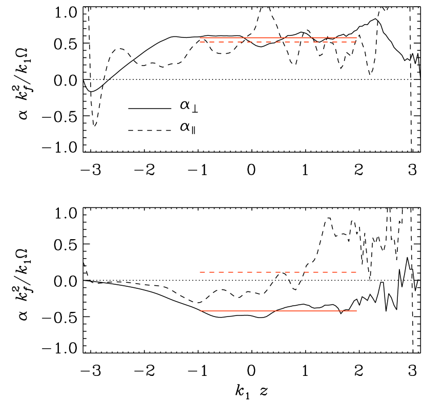
Figure 1.— Comparison of $\alpha_{\perp}$ (solid) and $\alpha_{\parallel}$ (dashed) for the runs with $\lambda^{(u)}=0.33$ (upper panel) and 0.61 (lower panel).

In Figure 1, we plot the normalized profiles of $\tilde{\alpha}_{\perp}\equiv\alpha_{\perp}k_{\it f}^{2}/k_{1}\Omega$ and $\tilde{\alpha}_{\parallel}\equiv\alpha_{\parallel}k_{\it f}^{2}/k_{1}\Omega$ as functions of $z$. Note that within the range $z_{1}\leq z\leq z_{2}$ with $k_{1}z_{1}=-1$ and $k_{1}z_{2}=2$, both functions are approximately constant. For $\lambda^{(u)}\mathrel{\mathchoice{\vbox{\offinterlineskip\halign{\hfil$\displaystyle#$\hfil\cr>\cr\sim\cr}}}{\vbox{\offinterlineskip\halign{\hfil$\textstyle#$\hfil\cr>\cr\sim\cr}}}{\vbox{\offinterlineskip\halign{\hfil$\scriptstyle#$\hfil\cr>\cr\sim\cr}}}{\vbox{\offinterlineskip\halign{\hfil$\scriptscriptstyle#$\hfil\cr>\cr\sim\cr}}}}0.5$, they are of opposite sign; see the lower panel of Figure 1 and Table LABEL:Tresults. As discussed above, this behavior has been seen and interpreted in earlier calculations (Brandenburg et al., 1990; Ferrière, 1992; Rüdiger & Kichatinov, 1993).

Figure 2.— Dependence of the normalized mean values of $\alpha_{\perp}$ on the value of $\lambda^{(u)}$ for $\mbox{\rm Co}=0.15$ (upper panel) and 0.4 (lower panel), giving respectively $\sigma\approx 1/2$ and $\approx 1/3$ as the zeros in each graph.

In Figure 2 we plot the dependence of the normalized mean values of $\alpha_{\perp}$ on the value of $\lambda^{(u)}$ for two values of Co. The value of $\sigma$ can then be read off as the zero of that graph. We find $\sigma\approx 1/2$ for low values of Co, and a somewhat smaller value ($\sigma\approx 1/3$) for larger values of Co.

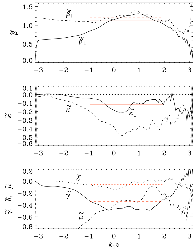
Figure 3.— Transport coefficients for the run with $\lambda^{(u)}=0.61$.

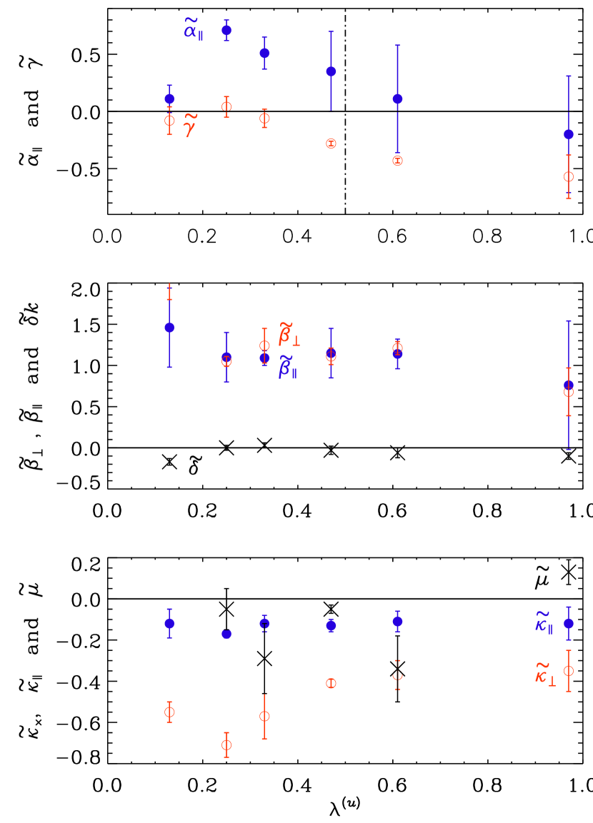
Figure 4.— Results for the other transport coefficients for $\mbox{\rm Co}=0.15$.

Table 1 Basic parameters and turbulent transport coefficients for the forced turbulence simulations.

$\mbox{\rm Re}_{M}$ Co $\lambda^{(u)}$ $\alpha_{\perp}k_{\it f}^{2}/\Omega k_{1}$ $\alpha_{\parallel}k_{\it f}^{2}/\Omega k_{1}$ $\gamma/\eta_{\rm t0}(z)k_{1}$ $\beta_{\perp}/\eta_{\rm t0}(z)$ $\beta_{\parallel}/\eta_{\rm t0}(z)$ $\delta/\eta_{\rm t0}(z)$ $\kappa_{\perp}/\eta_{\rm t0}(z)$ $\kappa_{\parallel}/\eta_{\rm t0}(z)$ $\mu/\eta_{\rm t0}(z)$ 70 0.14 0.13 $0.47\pm 0.16$ $0.1\pm 0.1$ $-0.1\pm 0.1$ $1.5\pm 0.2$ $2.1\pm 0.3$ $-0.2\pm 0.0$ $-0.1\pm 0.1$ $-0.6\pm 0.1$ $-1.8\pm 0.4$ 56 0.17 0.25 $0.82\pm 0.10$ $0.7\pm 0.1$ $0.0\pm 0.1$ $1.1\pm 0.1$ $1.0\pm 0.1$ $0.0\pm 0.0$ $-0.2\pm 0.0$ $-0.7\pm 0.1$ $-0.1\pm 0.1$ 62 0.16 0.33 $0.57\pm 0.03$ $0.5\pm 0.1$ $-0.1\pm 0.1$ $1.1\pm 0.2$ $1.2\pm 0.2$ $0.0\pm 0.0$ $-0.1\pm 0.0$ $-0.6\pm 0.1$ $-0.3\pm 0.2$ 47 0.20 0.46 $0.32\pm 0.26$ $0.2\pm 0.3$ $-0.2\pm 0.1$ $1.1\pm 0.2$ $1.0\pm 0.2$ $-0.0\pm 0.0$ $-0.1\pm 0.0$ $-0.4\pm 0.0$ $-0.1\pm 0.0$ 65 0.15 0.61 $-0.42\pm 0.06$ $0.1\pm 0.5$ $-0.4\pm 0.0$ $1.1\pm 0.1$ $1.2\pm 0.1$ $-0.1\pm 0.1$ $-0.1\pm 0.1$ $-0.4\pm 0.1$ $-0.3\pm 0.2$ 59 0.16 0.97 $-1.29\pm 0.26$ $-0.2\pm 0.5$ $-0.6\pm 0.2$ $0.8\pm 0.3$ $0.7\pm 0.3$ $-0.1\pm 0.0$ $-0.1\pm 0.1$ $-0.3\pm 0.1$ $0.1\pm 0.1$ 108 0.36 0.10 $0.20\pm 0.02$ $-0.1\pm 0.1$ $0.0\pm 0.0$ $0.9\pm 0.1$ $1.6\pm 0.2$ $0.1\pm 0.0$ $0.1\pm 0.0$ $-0.5\pm 0.1$ $-1.6\pm 0.2$ 93 0.41 0.14 $0.12\pm 0.04$ $-0.1\pm 0.0$ $-0.0\pm 0.0$ $1.0\pm 0.1$ $2.2\pm 0.4$ $0.0\pm 0.0$ $0.1\pm 0.0$ $-0.3\pm 0.1$ $-1.7\pm 0.4$ 75 0.51 0.35 $0.30\pm 0.05$ $0.3\pm 0.0$ $-0.2\pm 0.1$ $1.0\pm 0.1$ $0.8\pm 0.1$ $0.0\pm 0.0$ $-0.3\pm 0.0$ $-1.1\pm 0.0$ $0.2\pm 0.0$ 74 0.52 0.59 $-0.36\pm 0.02$ $0.2\pm 0.1$ $-0.7\pm 0.1$ $1.2\pm 0.0$ $0.8\pm 0.0$ $-0.3\pm 0.1$ $-0.2\pm 0.1$ $-0.9\pm 0.0$ $0.3\pm 0.0$

In Figure 3 we show the $z$-dependence of the remaining 7 normalized coefficients. They are all approximately independent of $z$ within the same range $z_{1}\leq z\leq z_{2}$ as before. In Figure 4 we show the scaling of these turbulent transport coefficients (including now also $\tilde{\alpha}_{\parallel}$) with $\lambda^{(u)}$. The results for $\alpha_{\parallel}$ and $\gamma$ suggest a dependence proportional to the gradient of $\overline{\rho}^{\sigma_{i}}u_{\rm rms}$ with $\sigma_{\alpha_{\parallel}}$ between 0 and 0.3 for $\alpha_{\parallel}$ and $\sigma_{\gamma}$ between 0.7 and 1 for $\gamma$. On the other hand, all the other coefficients seem to be independent of $\lambda$ and we find $\tilde{\beta}_{\parallel}\approx\tilde{\beta}_{\perp}\approx 1.1$, $\tilde{\delta}\approx 0$, $\tilde{\kappa}_{\parallel}\approx-0.1$, $\tilde{\kappa}_{\perp}\approx-0.4$, and $\tilde{\mu}\approx-0.05$. These results are quantitatively and qualitatively in agreement with those of Brandenburg et al. (2012). The fact that $\tilde{\delta}$ turned out to be essentially zero was addressed earlier (Brandenburg et al., 2012), where it was found that significant values are only found for scale separation ratios around unity, i.e., when the scale of the mean field is comparable to that of the turbulent eddies.

3.4. The case of supernova-driven ISM turbulence

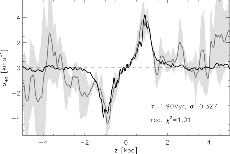
Figure 5.— Time-averaged vertical profile of $\alpha_{yy}$ from ISM turbulence (see Gressel, Elstner & Rüdiger, 2011), obtained with the test-field method (gray line). The best-fit model (black line) with $\sigma=0.327$ is obtained by method of least squares, weighted with the standard deviation (shaded area) in $\alpha_{yy}$.

We now turn to simulations of supernova-driven ISM turbulence (see Gressel et al., 2008a, b, for a detailed description of the model), similar to those of Korpi et al. (1999) and Gent et al. (2012), but extending to larger box sizes, thus allowing for better scale separation. In these simulations, expansion waves are driven via localized injection of thermal energy, $\Gamma_{\rm SN}(\bm{x},t)$. Additionally, optically thin radiative cooling with a realistic cooling function $\tilde{\Lambda}(T)$ and heating $\rho\Gamma(z)$ lead to a segregation of the system into multiple ISM phases.

Here we solve the visco-resistive compressible MHD equations (supplemented by a total energy equation), using the Nirvana-III code (Ziegler, 2004); for the full set of equations, we refer the reader to Equations (2.1) in Gressel (2010). For the present run, we chose a resolution of $128\times 128\times 512$ mesh points, and apply a value of $\mbox{\rm Pr}_{M}=2.5$. The fluid Reynolds number, defined as $\mbox{\rm Re}\equiv u_{\rm rms}\,\ell_{0}/(2\pi\nu)$, varies within the domain and takes values $\mbox{\rm Re}\simeq 70$–$165$, which is somewhat larger than for the forced turbulence case, where $\ell_{0}=2\pi/k_{\it f}$. The Coriolis number ${\rm Co}\equiv 2\Omega\tau_{0}$ is here $\simeq 0.24$.

Despite the aforementioned differences, the basic properties of the turbulence producing an $\alpha$ effect are in fact quite similar: rotation of the system together with stratification in the mean density and turbulence amplitude. Notably, the ISM simulations are strongly compressible with peak Mach numbers of up to ten, corresponding to a typical value of $\mu_{c}\simeq 1.9$, and with peak values up to five. We note that the ISM simulations also include shear with $S=-\Omega$, which may affect the production of vorticity.

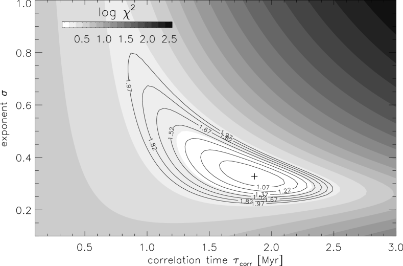
Figure 6.— Likelihood map based on the reduced-$\chi^{2}$ error estimate, with the best-fit parameter set indicated by the cross.

To obtain an estimate for $\sigma$ from the time-series of a single simulation run, we apply a method distinct from the one described above: We treat the $\alpha_{yy}(z)$ profile (inferred with test-field method I) as the data to be modeled and obtain error estimates by means of the standard deviation within four equal sub-intervals in time (see gray line and shaded areas in Figure 5). We then compute time averages of the profiles for $\mbox{\boldmath$\nabla$}{}\ln\overline{\rho}$ and $\mbox{\boldmath$\nabla$}{}\ln u_{\rm rms}$ (here without error estimates), from which we compute a model prediction for $\alpha_{yy}(z)$ based on the expression

$$\alpha_{yy}=-\tau_{\alpha}^{2}u_{\rm rms}^{2}\,\bm{\Omega}\cdot\mbox{\boldmath$\nabla$}{}\ln\left(\overline{\rho}^{\sigma}u_{\rm rms}\right),$$ (29)

where we have assumed that $\ell_{\alpha}$ can be replaced by $\tau_{\alpha}u_{\rm rms}(z)$, with $u_{\rm rms}(z)$ being the $z$-dependent rms velocity and $\tau_{\alpha}$ (assumed independent of $z$) is a characteristic timescale related to the $\alpha$ effect. We apply a least-square optimization allowing $\tau_{\alpha}$ and $\sigma$ as free parameters. The best-fit model according to Equation (29) is plotted as a black line in Figure 5, along with the stated values for $\tau_{\alpha}$ and $\sigma$, and matches well the data within the error bars.

Because we cannot a priori assure that $\tau_{\alpha}$ is uniform in space, and because this might affect the precise determination of $\sigma$, we perform an additional test. We do this by independently estimating $\ell_{0}(z)$ from the two-point velocity correlation function, computed in horizontal slabs around a given galactic height $z$, and time averaged over multiple snapshots. By comparing the obtained $\ell_{0}(z)$ with $u_{\rm rms}(z)$, we find that our data are broadly compatible with a uniform $\tau_{0}$ of about $1.2\,{\rm Myr}$. To corroborate the fit, we compute a likelihood map in the parameter space spanned by $\tau_{\alpha}$ and $\sigma$ and find that the best-fit parameter set is, in fact, located at the global minimum of the reduced-$\chi^{2}$ map; see Figure 6. The best-fit value of $\tau_{\alpha}$ is around $1.9\,{\rm Myr}$, which is indeed compatible with the correlation time $\tau_{0}$.

To conclude this section, we remark that we here find a somewhat smaller exponent, $\sigma\simeq 1/3$, which suggests that this case deviates from the theoretical prediction. It has however a similar exponent as in our stratified forced turbulence simulations with larger values of Co. Note that with the determined value for $\mu_{c}$, Equation (18) predicts a value of $\sigma\simeq 0.62$, which is a factor two larger than obtained from the fit. The reason for such discrepancy between the theoretical predictions and the simulations of supernova-driven ISM turbulence might be caused by the fact that the theory is developed for simplified conditions which are different from these simulations.

3.5. Convection-driven turbulence

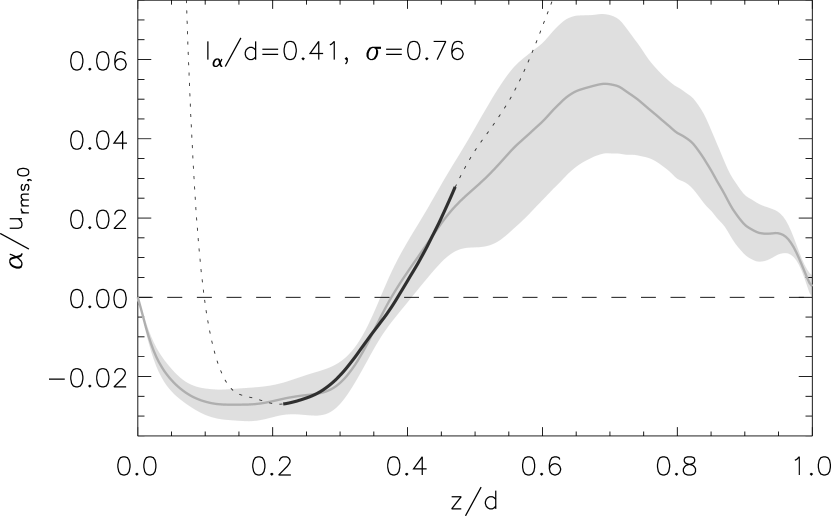
Figure 7.— Dependence of $\alpha$ on $z$ for convective turbulence without overshoot layers (gray line, with shaded areas indicating fluctuations) compared with Equation (2) (black line / dotted) applying $\sigma=0.76$ and $\ell_{\alpha}=0.41\,d$, as obtained from a least-square fit within the highlighted interval in $z/d$.

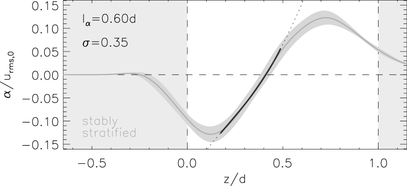
Figure 8.— Same as Figure 7, but the case with overshoot layers and weak temperature stratification, comparing $\alpha$ (gray line, shaded areas) measured via the test-field method with Equation (2) (black line / dotted) yielding $\sigma=0.35$ and $\ell_{\alpha}=0.6\,d$ as best-fit values.

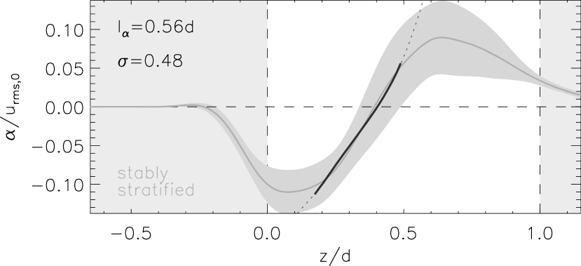
Figure 9.— Same as Figure 7, but the case with overshoot layers and stronger temperature stratification, comparing $\alpha$ (gray line, shaded areas) with Equation (2) using $\sigma=0.48$ and $\ell_{\alpha}=0.56\,d$ (black line / dotted).

Table 2Summary of convection runs.

Run Ra Ta $\Delta\overline{\rho}_{\rm total}$ $\Delta\overline{\rho}_{\rm CZ}$ overshoot Res. A $1.3\cdot 10^{6}$ $3.6\cdot 10^{5}$ 64 64 $-$ $256^{3}$ B $6.1\cdot 10^{5}$ $6.4\cdot 10^{4}$ 37 7 + $128^{3}$ C $6.1\cdot 10^{5}$ $6.4\cdot 10^{4}$ 290 296 + $128^{3}$

Many astrophysical bodies have turbulent convection zones. Again, rotation and stratification induce helicity into the flow and therefore drive an $\alpha$ effect. In stellar mixing length theory (Vitense, 1953), one assumes that the temperature fluctuation, $T^{\prime}$, is proportional to $u_{\rm rms}^{2}$, so the convective flux $\overline{(\rho\mbox{\boldmath$u$}{})^{\prime}c_{p}T^{\prime}}$ is well approximated by $\overline{\rho}u_{\rm rms}^{3}$, which is also confirmed by simulations (Brandenburg et al., 2005). In the steady state, the total energy flux is constant in space, so if most of the flux is carried by convection, then $\overline{\rho}u_{\rm rms}^{3}={\rm const}{}$ and thus its vertical gradient vanishes. If the scaling of Section 3.4 were applicable also to this case, i.e., if $\alpha\propto{\rm d}{}\ln\overline{\rho}u_{\rm rms}^{3}/{\rm d}{}z$, then $\alpha$ would vanish. To investigate this somewhat worrisome possibility, we now consider Now we consider a simulation of turbulent convection in a stratified layer, heated from below by a constant energy flux $\mbox{\boldmath$F$}{}_{\rm rad}$ at the bottom, where we adopt the diffusion approximation for an optically thick gas with $\mbox{\boldmath$F$}{}_{\rm rad}=-K\mbox{\boldmath$\nabla$}{}T$ and radiative conductivity $K$. We either consider a constant value of $\chi=K/(\rho c_{p})$ with an enhanced turbulent heat conductivity $\chi_{\rm t}$ near the surface as in spherical simulations of Käpylä et al. (2011), or, alternatively, a piecewise constant profile $K(z)$, such that ${\bm{g}}\cdot\mbox{\boldmath$\nabla$}{}s$ is positive in the middle of the domain, which corresponds to convective instability. The latter setup is described in detail in Käpylä et al. (2009). The hydrostatic equilibrium value of ${\bm{g}}\cdot\mbox{\boldmath$\nabla$}{}s$ is proportional to the Rayleigh number, Ra, which is here around $10^{6}$; see Käpylä et al. (2008) for the definition. The rotational influence is here measured in terms of the Taylor number $\mbox{\rm Ta}=(2\Omega d^{2}/\nu)^{2}$, which is $3.6\cdot 10^{5}$ for Run A. Summary of our convection simulations is given in Table LABEL:convectionruns. Run A without overshoot layers and $6.4\cdot 10^{3}$ for Runs B and C. Here $d$ is the thickness of the unstable layer. The density contrast, $\overline{\rho}_{\max}/\overline{\rho}_{\min}$, in the run without overshoot layers is 64. The vertical boundary conditions are stress-free and we use $\mbox{\rm Pr}_{M}=0.5$ and $\mbox{\rm Re}_{M}=52$ in Run A, and $\mbox{\rm Pr}_{M}=1$ and $\mbox{\rm Re}_{M}=13$ in Runs B and C. In Figure 7 we give the results for Run A without overshoot layers. The Coriolis number varies with height and is about 0.2 in the middle of the layer. The rotation axis is anti-parallel to the direction of gravity, corresponding thus to a location at the north pole. The system is therefore isotropic in the $xy$ plane and we consequently quote the mean between the two horizontal components, i.e., $\alpha={\textstyle{1\over 2}}(\alpha_{xx}+\alpha_{yy})$, using test-field method I, which corresponds to $\alpha_{\perp}$ of test-field method II. Note that in this simulation, $\alpha(z)$ shows a sinusoidal profile, suggestive of either weak stratification or effects of boundaries. Given that density stratification is not small (the density contrast is 64), it is plausible that the effects of boundaries are here responsible for the extended regime with negative $\alpha$.

Our simulation shows that the best fit is obtained for $\sigma\approx 0.75$. A possible reason for this unexpected behavior might be poorer scale separation in convection simulations compared with forced turbulence simulations. The other possibility is related to the absence of convective overshoot layers discussed above. This idea is partly confirmed by comparing with simulations that include convective overshoot layers. Now the best fit value for $\sigma$ is found to be about 1/3 when the temperature stratification is weak (Figure 8) and about 1/2 when the temperature stratification is strong (Figure 9).

Table 3Summary of results for $\sigma$.

Co $\overline{\rho}_{\max}/\overline{\rho}_{\min}$ $\sigma$ forced turbulence 0.15 535 1/2 0.40 535 1/3 supernova-driven ISM 0.24 1000 1/3 convective turbulence (CT) 0.2 64 3/4 CT with overshoot 0.2 37 1/3 0.2 290 1/2 analytic theory 1/2

4. Conclusions

While the present investigations confirm the old result that the $\alpha$ effect in mean-field dynamo theory emerges as the combined action of rotation and stratification of either density or of turbulent intensity, they also now point toward a revision of the standard formula for $\alpha$. The old formula by Steenbeck et al. (1966) predicted that the effect of stratification can be subsumed into a dependence on the gradient of $\overline{\rho}u_{\rm rms}$. This formula was then generalized by Rüdiger & Kichatinov (1993) to a dependence on $\overline{\rho}^{\sigma}u_{\rm rms}$, where $\sigma=3/2$ in the high conductivity limit for slow rotation, and $\sigma=1$ for faster rotation. In contrast, our new results now clearly favor a value of $\sigma$ below unity. The idealized case of artificially forced turbulence can most directly be compared to our analytic derivation, since it agrees in all the made assumptions. The obtained value of $\sigma=1/2$ agrees very well with the theoretical expectation. A similar exponent is found for the case of turbulent convection with higher temperature stratification, but the results seem to depend sensitively on model parameters (see Table LABEL:summaryall). Here more detailed studies will be required. Moreover, the result $\sigma=1/2$ arises naturally from analytical considerations for large fluid and magnetic Reynolds numbers and slow rotation as the only tenable choice, but those considerations have not yet been performed for the cases of intermediate and rapid rotation.

Forced turbulence simulations show a trend toward smaller values of $\sigma$ around 1/3 for faster rotation and also in cases of supernova-driven turbulence. Turbulent convection with overshoot also gives 1/3 in one case of moderate temperature stratification with overshoot, while simulations without overshoot point toward values somewhat larger values around 3/4. However, in none of the cases we have found that the $\alpha$ effect diminishes to zero as a result of a trend toward constant convective flux for which $\overline{\rho}u_{\rm rms}^{3}$ is approximately constant. In spite of the considerable scatter of the values of $\sigma$ found from various simulations, it is worth emphasizing that in all cases $\sigma$ is well below unity. On theoretical grounds, the value 1/2 is to be expected. Except for the forced turbulence simulations that also yield 1/2 for slow rotation, all other cases are too complex to expect agreement with our theory that ignores, for example, inhomogeneities of the density scale height and finite scale separation.

Appendix A Identities used for the derivation of Equation (8)

To derive Equation (8) we use the following identities:

$$\overline{\rho}^{\sigma}\,\left[\mbox{\boldmath$\nabla$}{\bm{\times}}\left(\mbox{\boldmath$\nabla$}{\bm{\times}}{\bm{u}}\right)\right]_{i}=\left[\nabla_{i}^{(\lambda)}\nabla_{j}^{(\lambda)}-\delta_{ij}\,\big{(}\mbox{\boldmath$\nabla$}^{(\lambda)}\big{)}^{2}\right]V_{j},$$ (A1)

$$\overline{\rho}^{\sigma}\,\big{[}\mbox{\boldmath$\nabla$}{\bm{\times}}[\mbox{\boldmath$\nabla$}{\bm{\times}}({\bm{u}}{\bm{\times}}{\bm{\Omega}})]\big{]}_{i}=\left[\nabla_{i}^{(\lambda)}\nabla_{j}^{(\lambda)}-\delta_{ij}\,\big{(}\mbox{\boldmath$\nabla$}^{(\lambda)}\big{)}^{2}\right]$$

$$\quad\quad\times({\bm{V}}{\bm{\times}}{\bm{\Omega}})_{j},$$ (A2)

$$\left[\nabla_{i}^{(\lambda)}\nabla_{j}^{(\lambda)}-\delta_{ij}\,\big{(}\mbox{\boldmath$\nabla$}^{(\lambda)}\big{)}^{2}\right]({\bm{V}}{\bm{\times}}{\bm{\Omega}})_{j}=\big{(}{\bm{\Omega}}{\bm{\times}}\mbox{\boldmath$\nabla$}^{(\lambda)}\big{)}_{i}(\mbox{\boldmath$\lambda$}{\bm{\cdot}}{\bm{V}})$$

$$\quad\quad+\big{(}{\bm{\Omega}}{\bm{\cdot}}\mbox{\boldmath$\nabla$}^{(\lambda)}\big{)}\big{(}\mbox{\boldmath$\nabla$}^{(\lambda)}{\bm{\times}}{\bm{V}}\big{)}_{i}.$$ (A3)

Equation (A3) is obtained by multiplying the identity

$$\varepsilon_{ijm}\Omega_{m}+\Omega_{l}\left(\varepsilon_{jml}\Lambda_{im}-\varepsilon_{iml}\Lambda_{jm}\right)=\varepsilon_{ijm}\Lambda_{ml}\Omega_{l},$$ (A4)

by $\Lambda^{2}V_{j}$, where $\varepsilon_{ijk}$ is the fully antisymmetric Levi-Civita tensor, $\Lambda_{mn}=\Lambda_{m}\Lambda_{n}/\Lambda^{2}$, and the identity (A4) is valid for arbitrary vectors ${\bm{\Omega}}$ and ${\bm{\Lambda}}$.

References

- Brandenburg & Dobler (2002) Brandenburg, A., & Dobler, W. 2002, Comp. Phys. Comm., 147, 471
- Brandenburg et al. (2005) Brandenburg, A., Chan, K. L., Nordlund, Å., & Stein, R. F. 2005, Astron. Nachr., 326, 681
- Brandenburg et al. (1990) Brandenburg, A., Nordlund, Å., Pulkkinen, P., Stein, R.F., & Tuominen, I. 1990, A&A, 232, 277
- Brandenburg et al. (2012) Brandenburg, A., Rädler, K.-H., & Kemel, K. 2012, A&A, 539, A35
- Brandenburg et al. (2008) Brandenburg, A., Rädler, K.-H., & Schrinner, M. 2008, A&A, 482, 739
- Brandenburg & Subramanian (2005) Brandenburg, A., & Subramanian, K. 2005, Phys. Rep., 417, 1
- Ferrière (1992) Ferrière, K. 1992, ApJ, 391, 188
- Gent et al. (2012) Gent F. A., Shukurov A., Fletcher A., Sarson G. R., Mantere M. J., 2012, arXiv:1206.6784
- Gressel (2010) Gressel O., 2010, PhD thesis, University of Potsdam, arXiv:1001.5187
- Gressel, Elstner & Rüdiger (2011) Gressel O., Elstner D., Rüdiger G., 2011, IAUS, 274, 348
- Gressel et al. (2008a) Gressel O., Ziegler U., Elstner D., Rüdiger G., 2008a, AN, 329, 619
- Gressel et al. (2008b) Gressel O., Elstner D., Ziegler U., Rüdiger G., 2008b, A&A, 486, L35
- Hubbard & Brandenburg (2009) Hubbard, A., & Brandenburg, A. 2009, ApJ, 706, 712
- Käpylä et al. (2008) Käpylä, P. J., Korpi, M. J., & Brandenburg, A. 2008, A&A, 491, 353
- Käpylä et al. (2009) Käpylä, P. J., Korpi, M. J., & Brandenburg, A. 2009, A&A, 500, 633
- Käpylä et al. (2011) Käpylä, P. J., Mantere, M. J., & Brandenburg, A. 2011, Astron. Nachr., 332, 883
- Kichatinov (1991) Kichatinov, L.L. 1991, A&A, 243, 483
- Kitchatinov et al. (1994) Kitchatinov, L.L., Pipin V.V., & Rüdiger, G. 1994, Astron. Nachr., 315, 157
- Kleeorin & Rogachevskii (2003) Kleeorin, N., & Rogachevskii, I. 2003, Phys. Rev. E, 67, 026321
- Kleeorin et al. (1996) Kleeorin, N., Mond, M., & Rogachevskii, I. 1996, A&A, 307, 293
- Kleeorin et al. (1990) Kleeorin, N.I., Rogachevskii, I.V., & Ruzmaikin, A.A. 1990, Sov. Phys. JETP, 70, 878
- Korpi et al. (1999) Korpi, M. J., Brandenburg, A., Shukurov, A., Tuominen, I., & Nordlund, Å. 1999, ApJ, 514, L99
- Krause & Rädler (1980) Krause, F., & Rädler, K.-H. 1980, Mean-field Magnetohydrodynamics and Dynamo Theory (Oxford: Pergamon Press)
- McComb (1990) McComb, W.D. 1990, The Physics of Fluid Turbulence (Clarendon, Oxford)
- Moffatt (1978) Moffatt, H.K. 1978, Magnetic Field Generation in Electrically Conducting Fluids (Cambridge: Cambridge Univ. Press)
- Monin & Yaglom (1975) Monin, A.S. & Yaglom, A.M. 1975, Statistical Fluid Mechanics (MIT Press, Cambridge, Massachusetts)
- Orszag (1970) Orszag, S. A. 1970, J. Fluid Mech., 41, 363
- Parker (1979) Parker, E.N. 1979, Cosmical magnetic fields (Oxford University Press, New York)
- Pouquet et al. (1976) Pouquet, A., Frisch, U., & Léorat, J. 1976, J. Fluid Mech., 77, 321
- Rädler et al. (2003) Rädler, K.-H., Kleeorin, N., & Rogachevskii, I. 2003, Geophys. Astrophys. Fluid Dyn., 97, 249
- Roberts & Soward (1975) Roberts, P. H., & Soward, A. M. 1975, Astron. Nachr., 296, 49
- Rogachevskii & Kleeorin (2004) Rogachevskii, I., & Kleeorin, N. 2004, Phys. Rev. E, 70, 046310
- Rogachevskii et al. (2011) Rogachevskii, I., Kleeorin, N., Käpylä, P. J., Brandenburg, A., 2011, Phys. Rev. E, 84, 056314
- Rüdiger & Hollerbach (2004) Rüdiger, G., & Hollerbach, R. 2004, The magnetic universe (Wiley-VCH, Weinheim)
- Rüdiger & Kichatinov (1993) Rüdiger, G. & Kichatinov, L. L. 1993, A&A, 269, 581
- Ruzmaikin et al. (1988) Ruzmaikin, A., Shukurov, A., & Sokoloff, D. 1988, Magnetic Fields of Galaxies (Kluwer, Dordrecht)
- Schrinner et al. (2005) Schrinner, M., Rädler, K.-H., Schmitt, D., Rheinhardt, M., Christensen, U. 2005, Astron. Nachr., 326, 245
- Schrinner et al. (2007) Schrinner, M., Rädler, K.-H., Schmitt, D., Rheinhardt, M., Christensen, U. R. 2007, Geophys. Astrophys. Fluid Dyn., 101, 81
- Steenbeck et al. (1966) Steenbeck, M., Krause, F., & Rädler, K.-H. 1966, Z. Naturforsch., 21a, 369 376Berechnung der mittleren Lorentz-Feldstärke für ein elektrisch leitendes Medium in turbulenter, durch Coriolis-Kräfte beeinflußter Bewegung See also the translation in Roberts & Stix, The turbulent dynamo, Tech. Note 60, NCAR, Boulder, Colorado (1971).
- Vitense (1953) Vitense, E. 1953, Z. Astrophys., 32, 135
- Zeldovich et al. (1983) Zeldovich, Ya. B., Ruzmaikin, A. A., & Sokoloff, D. D. 1983, Magnetic Fields in Astrophysics (Gordon and Breach, New York)
- Ziegler (2004) Ziegler U., 2004, J. Comput. Phys., 196, 393