Precoder Design for Orthogonal Space-Time Block Coding based Cognitive Radio with Polarized Antennas

Abstract

The spectrum sharing has recently passed into a mainstream Cognitive Radio (CR) strategy. We investigate the core issue in this strategy: interference mitigation at Primary Receiver (PR). We propose a linear precoder design which aims at alleviating the interference caused by Secondary User (SU) from the source for Orthogonal Space-Time Block Coding (OSTBC) based CR. We resort to Minimum Variance (MV) approach to contrive the precoding matrix at Secondary Transmitter (ST) in order to maximize the Signal to Noise Ratio (SNR) at Secondary Receiver (SR) on the premise that the orthogonality of OSTBC is kept, the interference introduced to Primary Link (PL) by Secondary Link (SL) is maintained under a tolerable level and the total transmitted power constraint at ST is satisfied. Moreover, the selection of polarization mode for SL is incorporated in the precoder design. In order to provide an analytic solution with low computational cost, we put forward an original precoder design algorithm which exploits an auxiliary variable to treat the optimization problem with a mixture of linear and quadratic constraints. Numerical results demonstrate that our proposed precoder design enable SR to have an agreeable SNR on the prerequisite that the interference at PR is maintained below the threshold.

I Introduction

Cognitive Radio (CR) is an encouraging technology to combat the spectrum scarcity. In order to further enhance the spectrum utilization, the spectrum sharing strategy that Primary Users (PUs) and Secondary Users (SUs) coexist in licensed bands as long as PUs are preserved from the interference caused by SUs attracts much research efforts. Such a strategy is tantamount to a multi-user system in which the inter-user interference mitigation is the core. Various inter-user interference mitigation techniques for spectrum sharing CR systems have been put forward. They can be roughly grouped into two categories: power allocation [1]-[3] and precoding in Multiple-Input Multiple-Output (MIMO) CR systems [4]-[7].

Space Time Block Coding (STBC) exploits time and space diversity in MIMO systems so as to heighten the reliability of the message signal. Orthogonal STBC (OSTBC) are contrived in such a fashion that the vectors of coding matrix are orthogonal in both time and space dimensions. This feature yields a simple linear decoding at the receiver side so that no complex matrix manipulation—Singular Value Decomposition (SVD), for instance, is required for recovering the information bit from the gathered received symbols. Numerous precoding techniques have been mooted for unstructured codes. However, these techniques cannot be applied to OSTBC which should forcibly preserve a special space-time structure. The precoding design for OSTBC CR systems attracts less attention in previous work. Such previous work in [7] was based on the Maximum Likelihood (ML) space-time decoder, whereas the ML decoder is a nonlinear method. Inspired by Minimum Variance (MV) receiver applied for OSTBC multi-access systems [8] which used a weight matrix at the receiver side to quell the inter-user interference, we make use of MV approach to design a precoding matrix at Secondary Transmitter (ST).

The precoding matrix at ST is designed to comply with the needs in our CR system: maximizing the Signal to Noise Ratio (SNR) at Secondary Receiver (SR) on the premise that the orthogonality of OSTBC is kept, the interference introduced to Primary Link (PL) by Secondary Link (SL) is maintained under a tolerable level and the total transmitted power constraint at ST is satisfied.

The classic MV beamforming [9], [10] built an optimization problem which includes only one linear constraint, that cannot administer to the needs in our CR system. On the other hand, some precoder designs for CR systems [6] introduced a mixture of linear and quadratic constraints to the optimization problem which leads to iterative solutions with high computational complexity. For the purpose of contriving a precoder that applies to our CR system and provides an analytic solution with low computational cost, we moot an original precoder design algorithm: we first take advantage of an optimization problem which includes one linear constraint with the objective of preserving the orthogonality of OSTBC and making SL introduce minimal interference to PL for different combinations of the polarization mode at ST and SR. This optimization problem provides an analytic solution in terms of an auxiliary variable which is the system gain on SL. Then we regulate this auxiliary variable using the quadratic constraints evoked by the transmitted power budget at ST and the maximum tolerable interference at Primary Receiver (PR). The polarization mode at ST and SR are conclusively settled on based upon the maximization criteria of SNR at SR.

The rest of the paper is organized as follows. The system model and OSTBC are presented in Section II. In Section III, we introduce the proposed precoder design for OSTBC based CR with polarized antennas. We report the numerical results and provide insights on the expected performance in Section IV. Finally, we give the conclusion in Section V.

II System Descriptions

We consider a CR system that consists of one SL which exploits OSTBC and one PL. ST and PT are only allowed to communicate with their peers. ST or PT is equipped with $N_{t}$ antennas and SR or PR is equipped with $N_{r}$ antennas. The antennas in the same array have identical polarization mode. On each link, the transmit antenna array or the receive antenna array is able to switch its polarization mode between vertical mode $V$ and horizontal mode $H$. We denote by $qt$ and $qr$, respectively, the transmit antenna array’s polarization mode and the receive antenna array’s polarization mode.

II-A System Model

In this paper, we exploit 3GPP Spatial Channel Model (SCM) [11]. The space channel impulse response between a pair of antennas $u$ and $s$ of path $n$ can be expressed as a function in terms of the polarization channel response and the geometric configuration of the antennas at both sides of the link:

$$H_{u,s,n}\left(\chi_{BS}^{\left(v\right)},\chi_{BS}^{\left(h\right)},\chi_{MS}^{\left(v\right)},\chi_{MS}^{\left(h\right)},\theta_{n,m,AoD},\theta_{n,m,AoA}\right)$$ (1)

where $\chi_{BS}^{\left(v\right)}$ is the BS antenna complex response for the V-pol component, $\chi_{BS}^{\left(h\right)}$ is the BS antenna complex response for the H-pol component, $\chi_{MS}^{\left(v\right)}$ is the MS antenna complex response for the V-pol component, $\chi_{MS}^{\left(h\right)}$ is the MS antenna complex response for the H-pol component, $\theta_{n,m,AoD}$ is the Angle of Departure (AOD) for the $m$th subpath of the $n$th path and $\theta_{n,m,AoA}$ is the Angle of Arrival (AOA) for the $m$th subpath of the $n$th path.

We assume that the system is operated over a frequency-flat channel with $N_{path}$ paths and each path contains only one subpath. For a point to point communication link, the baseband input-output relationship at time-slot $t$ is expressed as:

$$\mathbf{y}\left(t\right)=\sqrt{\frac{\rho}{N_{t}}}\mathbf{H}^{qt,qr}\mathbf{x}\left(t\right)+\mathbf{n}\left(t\right)$$ (2)

where $\rho$ is the SNR at each receive antenna, $\mathbf{x}\left(t\right)$ is a $N_{t}\times 1$ size transmitted signal vector which satisfies $E\left\{\mathbf{x}\left(t\right)\mathbf{x^{\mathit{H}}}\left(t\right)\right\}=N_{t}$, $\mathbf{n}_{j}(t)$ is a $N_{r}\times 1$ size complex Gaussian noise vector at receiver with zero-mean and unit-variance and $\mathbf{H}^{qt,qr}$ is the $N_{r}\times N_{t}$ channel matrix for the specified $qt$ and $qr$ with the entry

$$H_{u,s}^{qt,qr}=\sum_{n=1}^{N_{path}}H_{u,s,n}\left(\chi_{BS}^{\left(x\neq qt\right)}=0,\,\chi_{MS}^{\left(y\neq qr\right)}=0\right)$$ (3)

where $x,y\in\left\{V,\,H\right\}$. $\mathbf{H}^{qt,qr}$ has unit variance and satisfies $E\left\{\mathrm{tr\left(\mathbf{\mathbf{H}^{\mathit{qt,qr}}}\mathbf{\mathbf{H}^{\mathit{qt,qr}}}^{\mathrm{\mathit{H}}}\right)}\right\}=N_{t}N_{r}$.

Assuming that the channel is constant from $t=1$ to $t=T$, then Equation (2) can be extended into:

$$\mathbf{Y}=\sqrt{\frac{\rho}{N_{t}}}\mathbf{\mathbf{H}^{\mathit{qt,qr}}}\mathbf{X}+\mathbf{N}$$ (4)

where $\mathbf{Y}=\left[\mathbf{y}(1),\ldots,\mathbf{y}(T)\right]$, $\mathbf{X}=\left[\mathbf{x}(1),\ldots,\mathbf{x}(T)\right]$ and $\mathbf{N}=\left[\mathbf{n}\left(1\right),\ldots,\mathbf{n}\left(T\right)\right]$.

II-B Orthogonal Space-Time Block Coding

If $\mathbf{X}$ is OSTBC matrix, then $\mathbf{X}$ has a linear representation in terms of complex information symbols prior to space-time encoding $s_{k},\,k=1,\ldots,K$ [12]:

$$\mathbf{X}=\sum_{k=1}^{K}\left(\mathbf{C}_{k}\mathrm{Re}\left\{s_{k}\right\}+\mathbf{D}_{k}\mathrm{Im}\left\{s_{k}\right\}\right)$$ (5)

where $\mathbf{C}_{k}$ and $\mathbf{D}_{k}$ are $N_{t}\times T$ code matrices [13].

OSTBC matrix has the following unitary property:

$$\mathbf{X}\mathbf{X}^{H}=\left(\sum_{k=1}^{K}\left|s_{k}\right|^{2}\right)\mathbf{I}_{N_{t}\times N_{t}}$$ (6)

In order to represent the relationship between the original symbols and the received signal by multiplication of matrices, we introduce the “underline” operator [13] to rewrite Equation (2) as:

$$\mathbf{\underline{Y}}=\mathbf{\mathcal{\mathbb{\mathcal{H}}}}^{qt,qr}\mathbf{A}\mathbf{\mathrm{\mathbf{\underline{s}}}}+\underline{\mathbf{N}}$$ (7)

where $\mathbf{s}=\left[s_{1},\ldots,s_{K}\right]$ is the data stream which is QPSK modulated in this paper, $\mathbb{\mathcal{H}}^{qt,qr}=\left[\begin{array}[]{cc}\mathrm{Re}\left\{\mathbf{I}_{T}\otimes\mathbf{H}^{qt,qr}\right\}&\mathrm{-Im}\left\{\mathbf{I}_{T}\otimes\mathbf{H}^{qt,qr}\right\}\\ \mathrm{Im}\left\{\mathbf{I}_{T}\otimes\mathbf{H}^{qt,qr}\right\}&\mathrm{Re}\left\{\mathbf{I}_{T}\otimes\mathbf{H}^{qt,qr}\right\}\end{array}\right]$ is the equivalent channel matrix with the specified polarization mode, $\mathbf{A}=\left[\underline{\mathbf{C}_{1}},\ldots,\underline{\mathbf{C}_{k}},\underline{\mathbf{D}_{1}},\ldots,\underline{\mathbf{D}_{k}}\right]$ is the OSTBC compact dispersion matrix and the “underline” operator for any matrix $\mathbf{P}$ is defined as:

$$\underline{\mathbf{P}}\triangleq\left[\begin{array}[]{c}\mathrm{vec}\left\{\mathrm{Re}\left(\mathbf{P}\right)\right\}\\ \mathrm{vec}\left\{\mathrm{Im}\left(\mathbf{P}\right)\right\}\end{array}\right]$$ (8)

where $\mathrm{vec}\left\{\bullet\right\}$ is the vectorization operator stacking all columns of a matrix on top of each other.

The earliest OSTBC scheme which is well known as Alamouti’s code was proposed in [14]. Alamouti’s code gives full diversity in the spatial dimension without data rate loss. The transmission matrix of Alamouti’s code $C_{2}$ is given as:

$$C_{2}=\left[\begin{array}[]{cc}s_{1}&s_{2}\\ -s_{2}^{*}&s_{1}^{*}\end{array}\right]$$ (9)

In [15], Alamouti’s code was extended for more antennas. For instance, four antennas, the transmission matrix of the half rate code $C_{4}$ is given as:

$$C_{4}=\left[\begin{array}[]{cccc}s_{1}&s_{2}&s_{3}&s_{4}\\ -s_{2}&s_{1}&-s_{4}&s_{3}\\ -s_{3}&s_{4}&s_{1}&-s_{2}\\ -s_{4}&-s_{3}&s_{2}&s_{1}\\ s_{1}^{*}&s_{2}^{*}&s_{3}^{*}&s_{4}^{*}\\ -s_{2}^{*}&s_{1}^{*}&-s_{4}^{*}&s_{3}^{*}\\ -s_{3}^{*}&s_{4}^{*}&s_{1}^{*}&-s_{2}^{*}\\ -s_{4}^{*}&-s_{3}^{*}&s_{2}^{*}&s_{1}^{*}\end{array}\right]$$ (10)

III Precoder for OSTBC based CR with Polarized Antennas

We design a precoding matrix at ST which acts on the entry of the OSTBC compact dispersion matrix and has no influence on the codes’ structure. Our precoder design relies on the equivalent transmit correlation matrix on the link between ST and PR (SPL). This matrix can be estimated easily by SU in the sensing step and enables our precoder design to regulate the interference introduced by SL to PL.

III-A Constraints from SL

With the precoding operation, the received signal at SR for the specified polarization mode at ST and SR can be expressed as:

$$\underline{\mathbf{Y_{\mathit{ST,SR}}^{\mathit{qt,qr}}}}=\sqrt{\frac{\rho_{SR}}{N_{t}}}\mathbb{\mathcal{H}}_{ST,SR}^{qt,qr}\mathbf{W}^{qt,qr}\mathbf{A}\mathbf{\underline{s}}+\underline{\mathbf{N}}$$ (11)

where $\rho_{SR}$ is the SNR at each receive antenna of SR, $\mathbb{\mathcal{H}}_{ST,SR}^{qt,qr}$ is the SL equivalent channel matrix with the specified polarization mode at ST and SR, $\mathbf{\mathbf{W}^{\mathit{qt,qr}}}$ is the precoding matrix for the specified polarization mode at ST and SR.

A straightforward approach to estimate the transmitted signal from ST is using the following soft output detector:

$$\mathbf{\underline{\hat{s}}} = \mathbf{A}^{T}\mathbb{\mathcal{H}}_{ST,SR}^{qt,qr^{T}}\underline{\mathbf{Y_{\mathit{ST,SR}}^{\mathit{qt,qr}}}}$$

$$= \sqrt{\frac{\rho_{SR}}{N_{t}}}\mathbf{A}^{T}\mathbb{\mathcal{H}}_{ST,SR}^{qt,qr^{T}}\mathbb{\mathcal{H}}_{ST,SR}^{qt,qr}\mathbf{\mathbf{W}^{\mathit{qt,qr}}}\mathbf{A}\mathbf{\underline{s}}+\mathbf{A}^{T}\mathbb{\mathcal{H}}_{ST,SR}^{qt,qr^{T}}\underline{\mathbf{N}}$$

The OSTBC structure conservation puts forward the following constraint:

$$\mathbf{A}^{T}\mathbb{\mathcal{H}}_{ST,SR}^{qt,qr^{T}}\mathbb{\mathcal{H}}_{ST,SR}^{qt,qr}\mathbf{\mathbf{W}^{\mathit{qt,qr}}}\mathbf{A}=\alpha^{qt,qr}\mathbf{I}_{2K}$$ (13)

where $\alpha^{qt,qr}$ is the system gain on SL for the specified polarization mode at ST and SR which will be adjusted to satisfy the other constraints.

Additionally, the transmitted power budget at ST induces another constraint:

$$P_{t}^{qt,qr}\leq P_{tmax}$$ (14)

where $P_{t}^{qt,qr}=\frac{\rho_{SR}}{N_{t}}\mathrm{tr}\left(\mathbf{W^{\mathit{qt,qr}}}^{T}\mathbf{W}^{qt,qr}\right)$ and $P_{tmax}$ are, respectively, the transmitted power for the specified polarization mode at ST and SR and the maximum transmitted power at ST.

III-B Constraints from PL

The received signal at PR from ST is deemed as baleful signal by PL and can be expressed as:

$$\underline{\mathbf{Y_{\mathit{ST,PR}}^{\mathit{qt,qr^{\prime}}}}}=\sqrt{\frac{\rho_{PR}}{N_{t}}}\mathbb{\mathcal{H}}_{ST,PR}^{qt,qr^{\prime}}\mathbf{W}^{qt,qr}\mathbf{A}\mathbf{\underline{s}}+\underline{\mathbf{N}}$$ (15)

where $\rho_{PR}$ is the SNR at each receive antenna of PR and $\mathbb{\mathcal{H}}_{ST,PR}^{qt,qr^{\prime}}$ is the equivalent channel matrix for the specified polarization mode at ST and PR.

The interference power introduced by SL to PL for the specified polarization mode at ST and PR can be calculated as:

$$P_{ST,PR}^{qt,qr^{\prime}} = \mathrm{tr}\left[E\left(\mathbf{\underline{\mathbf{\mathbf{Y_{\mathit{ST,PR}}^{\mathit{qt,qr^{\prime}}}}}}}\,\mathbf{\underline{\mathbf{\mathbf{Y_{\mathit{ST,PR}}^{\mathit{qt,qr^{\prime}}}}}}}^{H}\right)\right]$$

$$= \frac{\rho_{SR}}{N_{t}}\mathrm{tr}\left(\mathbf{W^{\mathit{qt,qr}}}^{T}R_{\mathit{PR,ST}}^{\mathit{qt,qr^{\prime}}}\mathbf{W}^{qt,qr}\right)$$

where $\mathcal{R_{\mathit{PR,ST}}^{\mathit{qt,qr^{\prime}}}}=E\left(\mathbb{\mathcal{H}}_{PR,ST}^{qt,qr^{\prime}T}\mathbb{\mathcal{H}}_{PR,ST}^{qt,qr^{\prime}*}\right)$ is the equivalent transmit correlation matrix on SPL for the specified polarization mode at ST and PR. The maximum tolerable interference power $\eta$ at PR evokes the following constraint:

$$P_{ST,PR}^{qt,qr^{\prime}}\leq\eta$$ (17)

III-C Minimum Variance Algorithm

SU can dominate the configuration of the precoding matrix and the polarization mode on SL, while SU has no eligibility to select the polarization mode on PL. Our algorithm is based on an optimization problem which includes one linear constraint with the objective of preserving the orthogonality of OSTBC and making SL introduce minimal interference to PL for different combinations of the polarization mode at ST and SR. This optimization problem provides an analytic solution in terms of an auxiliary variable which is the system gain on SL. Then this auxiliary variable is regulated by using the quadratic constraints evoked by the transmitted power budget at ST and the maximum tolerable interference at PR. The polarization mode at ST and SR are conclusively settled on based upon the maximization criteria of SNR at SR.

Such an optimization problem that includes one linear constraint is described as follow:

$$\left(\widehat{\mathbf{W^{\mathit{qt,qr}}}},\,\widehat{qt},\,\widehat{qr}\right)=\arg\min_{\mathbf{W^{\mathit{qt,qr}}},\,qt,\,qr}\frac{\rho_{SR}}{N_{t}}\mathrm{tr}\left(\mathbf{W^{\mathit{qt,qr}}}^{T}\mathcal{R_{\mathit{PR,ST}}^{\mathit{qt,qr^{\prime}}}}\mathbf{W^{\mathit{qt,qr}}}\right)$$ (18)

$$\mathrm{subject}\;\mathrm{to}:\;\mathrm{tr}\left(\mathbf{A}^{T}\mathbb{\mathcal{H}}_{ST,SR}^{qt,qr^{T}}\mathbb{\mathcal{H}}_{ST,SR}^{qt,qr}\mathbf{\mathbf{W^{\mathit{qt,qr}}}}\mathbf{A}\mathit{\mathrm{-}}\alpha^{qt,qr}\mathbf{I}_{2K}\right)=0$$ (19)

We exploit the method of Lagrange multipliers to find $\widehat{\mathbf{W^{\mathit{qt,qr}}}}$ for each combination of the polarization mode at ST and SR. The Lagrangian function can be written as:

$$L\left(\mathbf{\mathbf{W^{\mathit{qt,qr}}}},\,\mathbf{\mathbf{\boldsymbol{\Lambda}}}\right) = \frac{\rho_{SR}}{N_{t}}\mathrm{tr}\left(\mathbf{\mathbf{W^{\mathit{qt,qr}}}}^{T}\mathcal{R_{\mathit{PR,ST}}^{\mathit{qt,qr^{\prime}}}}\mathbf{\mathbf{W^{\mathit{qt,qr}}}}\right)$$

$$-\mathrm{tr}\left(\mathbf{\mathbf{\boldsymbol{\Lambda}}}^{T}\left(\mathbf{A}^{T}\mathcal{R_{\mathrm{\mathit{ST,SR}}}^{\mathit{qt,qr}}}\mathbf{\mathbf{W^{\mathit{qt,qr}}}}\mathbf{A}\mathit{\mathrm{-}}\alpha^{qt,qr}\mathbf{I}_{2K}\right)\right)$$

(20)

where $\mathcal{R_{\mathrm{\mathit{ST,SR}}}^{\mathit{qt,qr}}}=\mathbb{\mathcal{H}}_{ST,SR}^{qt,qr^{T}}\mathbb{\mathcal{H}}_{ST,SR}^{qt,qr}$ and $\boldsymbol{\Lambda}$ is a $2K\times 2K$ size matrix of Lagrange multipliers.

By differentiating the Lagrange function with respect to $\mathbf{\mathbf{W^{\mathit{qt,qr}}}}$ and equating it to zero, we obtain an analytic solution in terms of $\alpha^{qt,qr}$ which is expressed as:

$$\widehat{\mathbf{W^{\mathit{qt,qr}}}}=\alpha^{qt,qr}\mathcal{R_{\mathit{PR,ST}}^{\mathit{qt,qr^{\prime}}}}^{-1}\mathcal{R_{\mathrm{\mathit{ST,SR}}}^{\mathit{qt,qr}}}\mathbf{A}\mathbf{Q^{\mathit{qt,qr}}}\mathbf{A}^{T}$$ (21)

where $\mathbf{Q^{\mathit{qt,qr}}}=\left(\mathbf{A}^{T}\mathcal{R_{\mathrm{\mathit{ST,SR}}}^{\mathit{qt,qr}}}\left(R_{\mathit{PR,ST}}^{\mathit{qt,qr^{\prime}}}\right)^{-1}\mathbf{A}\right)^{-1}$.

The estimated interference power at PR can be expressed in terms of $\alpha^{qt,qr}$ as:

$$\widehat{P_{ST,PR}^{qt,qr}}=\frac{\rho_{SR}\left(\alpha^{qt,qr}\right)^{2}\mathrm{tr}\left(\mathbf{Q^{\mathit{qt,qr}}}\right)}{N_{t}}$$ (22)

The estimated SNR at SR can be written in terms of $\alpha^{qt,qr}$ as:

$$\widehat{SNR_{ST,PR}^{qt,qr}}=\frac{\rho_{SR}\left(\alpha^{qt,qr}\right)^{2}\gamma^{qt,qr}}{N_{t}}$$ (23)

where

$$\gamma^{qt,qr}=$$

$$\mathrm{tr}\left(\mathbf{Q^{\mathit{qt,qr}}}\mathbf{A}^{T}\left(\mathcal{R_{\mathrm{\mathit{ST,SR}}}^{\mathit{qt,qr}}}R_{\mathit{PR,ST}}^{\mathit{qt,qr^{\prime}}}{}^{-1}\right)^{2}\mathcal{R_{\mathrm{\mathit{ST,SR}}}^{\mathit{qt,qr}}}\mathbf{AQ^{\mathit{qt,qr}}}\right)$$ (24)

.

The estimated transmit power at ST in terms of $\alpha^{qt,qr}$ is given by:

$$\widehat{P_{t}^{qt,qr}}=\frac{\rho_{SR}\left(\alpha^{qt,qr}\right)^{2}\delta^{qt,qr}}{N_{t}}$$ (25)

where

$$\delta^{qt,qr}=\mathrm{tr}\left(\mathbf{Q}^{qt,qr}\mathbf{A}^{T}\mathcal{R_{\mathrm{\mathit{ST,SR}}}^{\mathit{qt,qr}}}\left(R_{\mathit{PR,ST}}^{\mathit{qt,qr^{\prime}}}\right)^{-2}\mathcal{R_{\mathrm{\mathit{ST,SR}}}^{\mathit{qt,qr}}}\mathbf{AQ}^{qt,qr}\right)$$ (26)

We derive $\alpha^{qt,qr}$ by substituting $\widehat{P_{t}^{qt,qr}}$ and $\widehat{P_{ST,PR}^{qt,qr}}$ into Equation (14) and Equation (17) which indicate the transmitted power budget constraint and the maximum tolerable interference constraint:

$$\alpha^{qt,qr}=\min\left(\sqrt{\frac{N_{t}}{\delta^{qt,qr}}},\,\sqrt{\frac{N_{t}\eta}{\rho_{SR}\mathrm{tr}\left(\mathbf{Q^{\mathit{qt,qr}}}\right)}}\right)$$ (27)

Therefore the estimated SNR at SR can be determined as:

$$\widehat{SNR_{ST,PR}^{qt,qr}}=\min\left(\frac{\rho_{SR}}{\delta^{qt,qr}},\frac{\eta}{\mathrm{tr}\left(\mathbf{Q}^{\mathit{qt,qr}}\right)}\right)\gamma^{qt,qr}$$ (28)

Based upon the maximization criteria of SNR at SR, Finally, we destine the estimated polarization mode of ST and SR as:

$$\left(\widehat{qt},\widehat{qr}\right)=\arg\max_{qt,qr}\left[\min\left(\frac{\rho_{SR}}{\delta^{qt,qr}},\frac{\eta}{\mathrm{tr}\left(\mathbf{Q}^{qt,qr}\right)}\right)\gamma^{qt,qr}\right]$$ (29)

IV Numerical Results

For the purpose of validating our proposed precoding design algorithm, we simulated our CR system using the proposed precoder design algorithm and measure the SNR at SR by using varying maximum transmitted power at ST and a reasonable interference threshold at PR.

We firstly carried out our simulation with Alamouti’s code at ST for different combinations of $qt$ and $qr$ on SL under different multipath scenarios. Then, we executed our simulation with different codes for different number of transmit antennas at ST based upon a determinate combination of $qt$ and $qr$ on SL and multipath scenario. In both simulation scenarios, the Signal to Interference plus Noise Ratio (SINR) threshold to perceive the received signal at PR was chosen equal to $0\mathrm{dB}$ and the Cross-polar Discrimination (XPD) was set to $8\mathrm{dB}$. The channel matrix on each link was modeled according to 3GPP SCM. Since the status of polarization at PR $qr^{\prime}$ is normally unidentified for SU, the equivalent transmit correlation matrix on SPL becomes random. This thereby results in a random SNR at SR. In our simulation, we calculated the SNR at SR in terms of the polarization tilt angle at PR by introducing a rotation matrix to the equivalent transmit correlation matrix on SPL. We assumed that the polarization tilt angle at PR follows a continuous uniform distribution between $0$ and $\frac{\pi}{2}$. Then we sampled uniformly over the range of the polarization tilt angle at PR and calculated the SNR at SR for each sample of tilt angle. Finally, we worked out an average the SNR at SR to evaluate the system performance.

IV-A Performance Analysis of Polarization Diversity

We simulated a CR system, where ST is equipped with 2 antennas, SR is equipped with 1 antenna and PR is equipped with 2 antennas. We observe the variation of the average SNR at SR for different combinations of $qt$ and $qr$ on SL as the transmit power at ST increases. First, we set SL channel as a 2-path frequency flat fading channel and SPL channel as a single path frequency flat fading channel. The variation tendencies in this scenario were depicted in Fig.1. Then we reset SPL channel as a 4-path frequency flat fading channel and the corresponding variation tendencies were shown in Fig.2. The average SNR at SR for a large number of samples leads to the smooth curves. As the transmit power at ST increases, the average SNR at SR of all different combinations of $qt$ and $qr$ on SL exhibit uptrend in both scenarios and linear increase is obtained when $P_{maxSU}/P_{noise}$ are below $15\mathrm{dB}$ in both scenarios, where $P_{noise}$ denotes the noise power at SR. The mismatch of $qt$ and $qr$ on SL induces a $15\mathrm{dB}$ gap between the matched modes and the mismatched modes when the average SNR at SR has linear increase in the first scenario. When we enhanced the number of paths in SPL channel, the average SNR at SR for the mismatched modes was declined by $6\mathrm{dB}$ and the gap was enlarged in the second scenario.

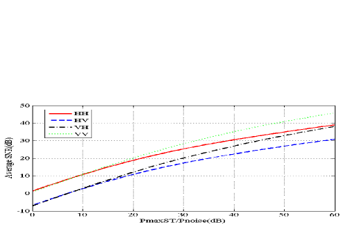
Figure 1: Average SNR at SR versus $P_{maxSU}/P_{noise}$ for different polarization mode on SL under single path scenario

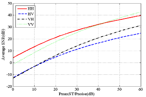
Figure 2: Average SNR at SR versus $P_{maxSU}/P_{noise}$ for different polarization mode under four paths scenario

IV-B Performance Analysis of Transmit Antennas Diversity

In the second simulation, we aimed to observe the average SNR at SR by using different number of transmit antennas. In the first circumstance, 2 transmit antennas and Alamouti’s code $C_{2}$ were utilized at ST. In the second circumstance, 4 transmit antennas and the half rate code $C_{4}$ were utilized at ST. In both circumstances, we set $qt=V$ and $qr=V$. SR is equipped with 1 antenna and PR is equipped with 4 antennas. The number of paths is chosen equal to 2 on SL and 6 on SPL.

For the case of 2 transmit antennas at ST, the SNR at SR reaches the saturation point at $20\mathrm{dB}$ when $P_{maxSU}/P_{noise}$ achieves $40\mathrm{dB}$. Compare to the previous results in Fig. 1 and 2, the SNR at SR reaches the saturation point faster due to the increase in number of paths on the SPL. However, the increase in number of antennas will significantly delay the arrival of the saturation point even the number of paths on the SPL is also increased. For the case of 4 transmit antennas at ST, the SNR at SR reaches the saturation point at $65\mathrm{dB}$ when $P_{maxSU}/P_{noise}$ achieves $100\mathrm{dB}$.

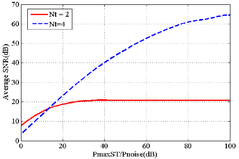
Figure 3: Average SNR at SR versus $P_{maxSU}/P_{noise}$ for different number of transmit antennas at ST

V Conclusions

A linear precoder design which aims at alleviating the interference at PR for OSTBC based CR has been introduced. One of the principal contributions is to endow the conventional prefiltering technique with the excellent features of OSTBC in the context of CR. The prefiltering technique has been optimized for the purpose of maximizing the SNR at SR on the premise that the orthogonality of OSTBC is kept, the interference introduced to PL by SL is maintained under a tolerable level and the total transmitted power constraint is satisfied. Numeral Results have shown that polarization diversity contributes to achieve better SNR at SR, moreover, the increase in number of antennas will significantly delay the arrival of the saturation point for the SNR at SR.

References

• [1] Y.-C. Liang, K.-C. Chen, G.-Y. Li, P. Mahonen, ”Cognitive Radio Networking and Communications: An Overview,” IEEE Trans. Vehicular Technology, vol. 60, no. 7, pp. 3386-3407, Sept. 2011.
• [2] A. Hoang, Y. Liang, and M. Islam, β€œPower control and channel allocation in cognitive radio networks with primary users’ cooperation,” IEEE Trans. Mobile Comput., vol. 9, no. 3, pp. 348–360, Mar. 2010.
• [3] R.-C. Xie, F.-R. Yu, H. Ji, β€œDynamic Resource Allocation for Heterogeneous Services in Cognitive Radio Networks With Imperfect Channel Sensing,” IEEE Trans. Vehicular Technology, vol. 61, no. 2, pp. 770 - 780, Feb. 2012.
• [4] R. Prasad and A. Chockalingam, β€œPrecoder Optimization in Cognitive Radio with Interference Constraints,” in Proc. IEEE ICC 2011.
• [5] M. Jung, K. Hwang, and S. Choi, β€œInterference Minimization Approach to Precoding Scheme in MIMO-Based Cognitive Radio Networks,” IEEE Commun. Lett., vol. 15, no. 8, pp. 789-791, Aug. 2011.
• [6] K. T. Phan, S. A. Vorobyov, N. D. Sidiropoulos, and C. Tellambura, β€œSpectrum sharing in wireless networks: A QoS-aware secondary multicast approach with worst user performance optimization,” in Proc. IEEE SAM’08, Jul. 2008, pp. 23–27.
• [7] A. Punchihewa, V.-K. Bhargava, C. Despins, β€œLinear Precoding for Orthogonal Space-Time Block Coded MIMO-OFDM Cognitive Radio,” IEEE Trans. Commun., vol. 59, no. 3, pp. 767-779, Mar. 2011.
• [8] S. Shahbazpanahi, M. Beheshti, A. B. Gershman, M. GharaviAlkhansari, and K. M. Wong, β€œMinimum variance linear receivers for multiaccess MIMO wireless systems with space–time block coding,” IEEE Trans. Signal Process., vol. 52, no. 12, pp. 3306–3313, Dec. 2004.
• [9] R. G. Lorenz and S. P. Boyd, β€œRobust minimum variance beamforming,” IEEE Trans. Signal Process., vol. 53, no. 5, pp. 1684–1696, May 2005.
• [10] C. D. Richmond, β€œCapon algorithm mean squared error threshold SNR prediction and probability of resolution,” IEEE Trans. Signal Process., vol. 53, no. 8, pp. 2748–2764, Aug. 2005
• [11] 3GPP TR 25.996 V10.0.0, β€œSpatial channel model for MIMO simulations,” www.3gpp.org, Mar. 2011.
• [12] R. L. G. Cavalcante and I. Yamada, β€œMultiaccess interference suppression in OSTBC-MIMO systems by adaptive projected subgradient method,” IEEE Trans. Signal Process., vol. 56, no. 3, pp. 1028–1042, Mar. 2008.
• [13] M. Gharavi-Alkhansari and A. B. Gershman, β€œConstellation space invariance of orthogonal space–time block codes,” IEEE Trans. Inf. Theory, vol. 51, no. 1, pp. 331–334, Jan. 2005.
• [14] S. M. Alamouti, β€œA simple transmit diversity technique for wireless communications,” IEEE J. Sel. Areas Commun., vol. 16, no. 8, pp. 1451–1458, Oct. 1998.
• [15] V. Tarokh, H. Javarkhani and Calderbank, β€œSpace-time block codes from orthogonal designs,” IEEE Transactions on Information Theory, vol. 45, no. 5, July 1999, pp. 1456-1467.