Functional renormalization group with a compactly supported smooth regulator function

Abstract:

The functional renormalization group equation with a compactly supported smooth (CSS) regulator function is considered. It is demonstrated that in an appropriate limit the CSS regulator recovers the optimized one and it has derivatives of all orders. The more generalized form of the CSS regulator is shown to reduce to all major type of regulator functions (exponential, power-law) in appropriate limits. The CSS regulator function is tested by studying the critical behavior of the bosonized two-dimensional quantum electrodynamics in the local potential approximation and the sine-Gordon scalar theory for $d<2$ dimensions beyond the local potential approximation. It is shown that a similar smoothing problem in nuclear physics has already been solved by introducing the so called Salamon-Vertse potential which can be related to the CSS regulator.

1 Introduction

The functional renormalization group (RG) method has been developed in order perform renormalization non-perturbatively, i.e. to determine the underlying exact low-energy effective theory without using perturbative treatments [1, 2, 3, 4, 5]. The functional RG equation in its most general form (for scalar fields) [3]

$$k\partial_{k}\Gamma_{k}[\phi]=\frac{1}{2}{\rm Tr}\left[(k\partial_{k}R_{k})/(\Gamma_{k}^{(2)}[\phi]+R_{k})\right]$$ (1)

is derived for the blocked effective action $\Gamma_{k}$ which interpolates between the bare $\Gamma_{k\to\Lambda}=S$ and the full quantum effective action $\Gamma_{k\to 0}=\Gamma$ where $k$ is the running momentum scale. The second functional derivative of the blocked action is represented by $\Gamma_{k}^{(2)}$ and the trace Tr stands for the momentum integration. $R_{k}$ is an appropriately chosen regulator function which fulfills the following requirements, $R_{k}(p\to 0)>0$, $R_{k\to 0}(p)=0$ and $R_{k\to\Lambda}(p)=\infty$. Since the RG equations are functional partial differential equations it is not possible to solve them in general, hence, approximations are required. One of the commonly used systematic approximation is the truncated derivative (i.e. gradient) expansion where the blocked action is expanded in powers of the derivative of the field,

$$\Gamma_{k}[\phi]=\int_{x}\left[V_{k}(\phi)+Z_{k}(\phi)\frac{1}{2}(\partial_{\mu}\phi)^{2}+...\right].$$ (2)

In the local potential approximation (LPA), i.e. in the leading order of the derivative expansion (2), higher derivative terms are neglected and the wave-function renormalization is set equal to constant, i.e. $Z_{k}\equiv 1$. The solution of the RG equations sometimes requires further approximations, e.g. the potential can be expanded in powers of the field variable. Since the approximated RG flow depends on the choice of the regulator function, i.e. on the renormalization scheme, the physical results (such as fixed points, critical exponents) could become scheme-dependent.

Therefore, a general issue is the comparison of results obtained by various RG schemes (i.e. various types of regulator functions) [6, 7, 10, 9, 8, 11, 14, 12, 15, 13, 16]. In order to optimize the scheme-dependence and to increase the convergence of the truncated flow (expanded in powers of the field variable), a general optimization procedure has already been worked out [6, 10] and the link between the optimal convergence and global stability of the flows was also discussed. Optimization scenarios has also been discussed in detail in [9]. Moreover, optimization through the principle of minimal sensitivity were also considered [13]. In the leading order of the derivative expansion (2), i.e. in LPA, an explicit form for the optimized (in a sense of [10]) regulator was provided [6] but it was also shown that this simple form of the optimized regulator does not support a derivative expansion beyond second order [9, 8, 6, 10]. The optimized regulator is a function of class $C^{0}$ with compact support thus it is a continuous function and it has a finite range but it is not differentiable. It was argued [6, 10] that beyond LPA a solution to the general criterion for optimization (see Eq.(5.10) of [10]) has to meet the necessary condition of differentiability to the given order.

In this work we give an example for a regulator function of class $C^{\infty}$ (it has derivatives of all orders, i.e. it is a smooth function) with compact support. We show that in an appropriate limit it recovers the optimized regulator (optimized in a sense of [6, 10]). Moreover, its generalized form can be considered as a prototype regulator which reduces to all major type of regulator functions (exponential, power-law) in appropriate limits. Finally, this regulator function is tested by studying the critical behavior of the bosonized two-dimensional quantum electrodynamics (QED₂) in LPA and the sine-Gordon scalar theory for $d<2$ dimensions beyond LPA.

2 Regulator functions

A large variety of regulator functions has already been discussed in the literature by introducing its dimensionless form

$$R_{k}(p)=p^{2}r(y),\hskip 14.22636pty=p^{2}/k^{2}$$ (3)

where $r(y)$ is dimensionless. For example, one of the simplest regulator function is the sharp-cutoff regulator

$$r_{{\mathrm{sharp}}}(y)=\frac{1}{\theta(y-1)}-1$$ (4)

where $\theta(y)$ is the Heaviside step function. The sharp-cutoff regulator has the advantage that the momentum integral in (1) can be performed analytically in the LPA. The corresponding RG equation is the Wegner-Houghton RG [1]. Its disadvantage is that it confronts to the derivative expansion, i.e. higher order terms (beyond LPA) cannot be evaluated unambiguously.

The compatibility with the derivetive expansion can be fulfilled by e.g. using an exponential type regulator function such as [3]

$$r_{{\mathrm{exp}}}(y)=\frac{c}{\exp\left(c_{2}y^{b}\right)-1}$$ (5)

with $b\geq 1$ and $c=1$ is a typical choice. The parameter $c_{2}$ can be chosen as e.g. $c_{2}=\ln(2)$. Let us note, the exponential regulator with $c\neq 0$, $c_{2}\neq\ln(2)$ has also been discussed in [13] using optimization through the principle of minimal sensitivity. Other exponential type regulators like, $r_{{\mathrm{mexp}}}=b/(\exp(cy)-1)$ with $c=\ln(1+b)$, $r_{{\mathrm{mod}}}=1/(\exp(c[y+(b-1)y^{b}]/b)-1)$ with $c=\ln(2)$, $r_{{\mathrm{mix}}}=1/(\exp(b[y^{a}-y^{-a}]/2a)-1)$ with $a\geq 0$ or $r_{{\mathrm{step}}}=(2b-2)y^{b-2}/(b[\exp(cy^{b-1})-1])$ with $c=\ln(3b-2)/b$ are also compatible with the derivative expansion [6]. Their disadvantage is that no analytic form can be derived for RG equations neither in LPA nor beyond. Thus, the momentum integral in (1) has to be performed numerically, and consequently, the dependence of the results on the upper bound of the numerical integration has to be considered.

The momentum integral of Eq. (1) can be performed analytically using the power-law type regulator [4]

$$r_{{\mathrm{pow}}}(y)=\frac{c}{y^{b}}$$ (6)

at least for $b=1$ and $b=2$ in LPA. Again $c=1$ is a typical choice. The power-law regulator is compatible with the derivative expansion (for any $b\geq 1$) but its disadvantage is that it is not ultraviolet (UV) safe for $b=1$ (at least not in all dimensions). One has to note that analyticity is lost beyond LPA. Therefore, similarly to the exponential type regulators, the dependence of the results on the upper bound of the numerical integration has to be considered.

Problems related to UV safety and the upper bound of the momentum integral can be handled by the optimized regulator function [6]

$$r_{{\mathrm{opt}}}(y)=\left(\frac{1}{y}-1\right)\theta(1-y)$$ (7)

which is a continuous function with compact support, thus the upper bound of the momentum integral in (1) is well-defined. A more general form of the optimized regulator reads

$$r_{{\mathrm{opt}}}^{{\mathrm{gen}}}(y)=c\left(\frac{1}{y^{b}}-1\right)\theta(1-y)$$ (8)

which was discussed in detail in the context of optimization through the principle of minimal sensitivity [13]. Furthermore, the momentum integral can be performed analytically in all dimensions in LPA and also if the wave function renormalization is included. Moreover, it was also shown that in LPA, the optimized regulator and the Polchinski RG [2] equation provides us the best results (closest to the exact ones) for the critical exponents of the O$(N)$ symmetric scalar field theory in $d=3$ dimensions [7]. This equivalence between the optimized and the Polchinski flows in LPA is the consequence of the fact that the optimized functional RG can be mapped by a suitable Legendre transformation to the Polchinski one in LPA [8] but this mapping does not hold beyond LPA. It was also shown [6] that the regulator (7) is a simple solution of the general criterion for optimization (see (5.10) of [10]) in LPA. Although, the regulator (7) is a continuous function but it is not differentiable and it was shown that it does not support the derivative expansion beyond second order. Indeed, it was argued in e.g. Ref. [10] that optimization has to meet the necessary condition of differentiability.

3 The CSS regulator function

Therefore, an appropriately chosen regulator which is a smooth function with compact support (it has derivatives of all orders and has a finite range) can handle problems related to UV safety and the upper bound of the momentum integration in all order of the derivative expansion. In this work we give an example for a compactly supported smooth (CSS) regulator which has the following general form

$$r_{{\mathrm{css}}}(y)=\frac{c_{1}}{\exp[c_{2}y^{b}/(1-y^{b})]-1}\theta(1-y)$$ (9)

with parameters $c_{1}$, $c_{2}$ and $b\geq 1$. Using the normalization $r_{{\mathrm{css}}}(y_{0})\equiv 1$ the CSS regulator reduces to

$$r_{{\mathrm{css}}}(y)=\frac{\exp[cy_{0}^{b}/(1-y_{0}^{b})]-1}{\exp[cy^{b}/(1-y^{b})]-1}\theta(1-y).$$ (10)

The regulator function (10) becomes exactly zero at $y=1$ and all derivatives of (10) are continuous everywhere.

It is important to note here a similar problem of nuclear physics. Nuclear states are often described by using single-particle basis states which are eigenstates of single-particle Hamiltonian with phenomenological nuclear potential of strictly finite range (SFR) character [17]. SFR potentials are zero at and beyond a finite distance. The most often used spherical potential, the Wood-Saxon potential becomes zero only at infinity, therefore, one has to cut the tail of this potential if one solves the Shroedinger equation numerically. The eigenstates however sometimes do depend on the cut-off radius [18]. In order to get rid off this dependence on the cut-off radius of the Wood-Saxon form, the so called Salamon-Vertse (SV) potential was proposed [18]. The SV potential becomes zero at a finite distance smoothly, moreover the SV form can be differentiated any times for non-zero distance. The SV potential is a linear combination of the function $f(r,\rho)=-e^{\frac{r^{2}}{r^{2}-\rho^{2}}}\theta(1-\rho)$ and its first derivative with respect to the radial distance $r$. The derivative term was added to make the SV potential be similar to the shape of the Wood-Saxon potential for heavy nuclei [19, 17]. For light nuclei one can safely use only the first term of the SV potential [21]. This term in a transformed form was used as a weight function

$$w(x)\sim\theta(1-|x|)~{}e^{\frac{1}{x^{2}-1}}$$ (11)

for having a finite range smoothing function for calculating the shell correction for weakly bound nuclei [20]. It is clear that

$$\frac{d^{n}w(x)}{dx^{n}}=0\quad\textrm{for}~{}|x|\geq 1~{}\textrm{and for}~{}n=0,1,2,..~{}.$$ (12)

Similar effect can be achived by using a class of functions satisfying the latter condition in (12). The present form of the CSS regulator falls into this class and it can be obtained from the SV potential. Similarly, the exponential regulator (5) is related to the Wood-Saxon potential.

In order to consider the criterion for optimization let us take the limit

$$\lim_{c\to 0}r_{{\mathrm{css}}}(y)=\frac{y_{0}^{b}}{1-y_{0}^{b}}\left(\frac{1}{y^{b}}-1\right)\theta(1-y)$$ (13)

which demonstrates that the CSS regulator (10) recovers the generalized form of the optimized regulator (8) and also shows that for the particular choice $y_{0}=1/2$ and $b=1$ the specified CSS regulator of the form

$$r_{{\mathrm{css}}}^{{\mathrm{spec}}}(y)=\frac{\exp(c)-1}{\exp[cy/(1-y)]-1}\theta(1-y)$$ (14)

recovers the optimized one (7) in the limit $c\to 0$. Thus, for small enough value for the parameter $c$, the specified CSS regulator (14) produces results closer to the those obtained by the optimized one (7) (the smaller the parameter $c$ the closer the critical exponents are). Let us note, however, that if $c$ is closer to zero higher derivates of (14) have sharp oscillatory peaks near $y=1$, thus the usage of the CSS regulator (14) in the limit $c\to 0$ requires careful numerical treatment at higher order of the derivative expansion. In case of an arbitrary value for $c$, the parameters $y_{0}$ and $b$ have to be redefined and the optimal choice can be done by using the criterion (5.10) of [10]. In general one finds $y_{0}(c)$ and $b(c)$ with the conditions $y_{0}(c\to 0)=1/2$ and $b(c\to 0)=1$. Let us note that the general criterion of optimization apart from (5.10) of [10], requires a supplementary constraint related to differentiabity, see (8.42) of [10]. It is illustrative to consider the case $y_{0}=1/2$, $b=1$ when these conditions can only be fulfilled by the specified CSS regulator if $c\to 0$. For $c\neq 0$ the determination of the optimized choice for $y_{0}$ and $b$ can only be done numerically in case of the CSS regulator which is not investigated in this work.

Let us rewrite the CSS regulator in a more general form

$$r_{{\mathrm{css}}}^{{\mathrm{gen}}}(y)=\frac{\exp[cy_{0}^{b}/(f-hy_{0}^{b})]-1}{\exp[cy^{b}/(f-hy^{b})]-1}\theta(f-hy^{b})$$ (15)

where two new parameters $f,h$ are introduced. If one takes the following limits

$$\lim_{f\to\infty}r_{{\mathrm{css}}}^{{\mathrm{gen}}}(y) = \frac{y_{0}^{b}}{y^{b}},$$ (16)

$$\lim_{h\to 0,c\to f}r_{{\mathrm{css}}}^{{\mathrm{gen}}}(y) = \frac{\exp[y_{0}^{b}]-1}{\exp[y^{b}]-1}$$ (17)

the generalized CSS regulator (15) reduces to the power-law (6) and to the exponential (5) regulators. Thus the the generalized CSS regulator (15) can be considered as a prototype regulator function which recovers all major types of regulator functions in appropriate limits.

Finally, let us note that a smooth regulator function with compact support has already been introduced in [16] and it reads

$$r(y)=\frac{1}{y}\exp\left[\frac{1}{y-c}\exp\left[\frac{1}{b-y}\right]\right]\theta(c-y)\theta(y-b)+\frac{1}{y}\theta(b-y).$$ (18)

Similarly to the CSS regulator (15) it has a finite range thus it can handle problems related to the upper bound of the momentum integral. However, it has an important disadvantage, namely that the regulator (18) in its present form is not suitable to recover the optimized one (7). For example, one can try to take the limits $c\to 1$, $b\to 0$ which result in a mixed type of regulator.

Therefore, comparing the two compact regulators (14) and (18), only the CSS regulator provides us a scheme to approximate a regulator which fulfills the general criterion for optimization [10] at any order of the derivative expansion. The usage of the CSS regulator at higher order of the derivative expansion requires considerable numerical efforts for small value of $c$ due to the sharp oscillatory peaks of higher derivates of (14) near $y=1$ but it is differentiable for $c\neq 0$, hence, it represents an approximation scheme to the optimized regulator in a sense of [10] at all orders of the derivative expansion.

4 Bosonized QED₂ and the CSS regulator

In order to test the specified CSS regulator function (14) let us study the critical behavior of the bosonized QED₂ which is the specific form of the massive sine-Gordon (MSG) model whose Lagrangian density is written as [11]

$${\cal{L}}_{\mathrm{MSG}}=\frac{1}{2}(\partial_{\mu}\varphi)^{2}+\frac{1}{2}M^{2}\varphi^{2}+u\cos(\beta\varphi)$$ (19)

with $\beta^{2}=4\pi$. The MSG model has two phases. The Ising-type phase transition [22] is controlled by the dimensionless quantity $u/M^{2}$ which separates the confining and the half-asymptotic phases of the corresponding fermionic model. The critical ratio which separates the phases of the model has been calculated by the density matrix RG method for the fermionic model and the most accurate result for the critical ratio is in the range [22]

$$\left[\frac{u}{M^{2}}\right]_{c}\in[0.156,0.168].$$ (20)

In the framework of functional RG in LPA the closest result to (20), i.e. the best result for the critical ratio reads $[u/M^{2}]_{c}=2/(4\pi)\approx 0.15915$. It can be determined by analytic considerations based on the infrared (IR) limit of the propagator, $\lim_{k\to 0}(k^{2}+V^{\prime\prime}_{k}(\varphi))=0$ where $V_{k}(\varphi)$ is the blocked scaling potential which contains the mass term and all the higher harmonics generated by RG transformations [12]. This result was reproduced by the optimized regulator (7) and also by the power-law type one (6) with $b=2$ [11]. However, if one considers the single Fourier-mode approximation (where $V_{k}(\varphi)$ contains the mass term and only a single cosine) the analytic result based on the IR behavior of the propagator gives $[u/M^{2}]_{c}=1/(4\pi)\approx 0.07957$ [12]. In this case only the optimized regulator (7) was able to produce a ratio $[u/M^{2}]_{c}=0.07964$ closer to the analytic one [11]. For example, RG flows obtained by power-law type regulators run into a singularity and stop at some finite momentum scale and the determination of the critical ratio was not possible [11]. Therefore, the usage of the single Fourier mode approximation provides us a tool to consider the convergence properties of the regulator functions.

In Fig. 1 the phase structure of the single-frequency MSG model (19) is shown which is obtained by the functional RG equation derived for the dimensionless blocked potential ($\tilde{V}_{k}=k^{-2}V_{k}$) for $d=2$ dimensions in LPA

$$(2+k\partial_{k}){\tilde{V}}_{k}(\varphi)=-\frac{1}{4\pi}\int_{0}^{\infty}dy\frac{y^{2}\frac{dr}{dy}}{(1+r)y+{\tilde{V}^{\prime\prime}}_{k}(\varphi)}$$ (21)

using the specified CSS regulator (14) with $c=0.1$. The tilde superscript denotes the dimensionless couplings, ${\tilde{M}}^{2}=k^{-2}M^{2}$ and ${\tilde{u}}_{k}=k^{-2}u_{k}$.

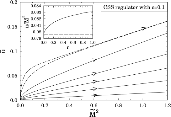
Figure 1: Phase diagram of the MSG model for $\beta^{2}=4\pi$ is obtained by the usage of the CSS regulator (14) with $c=0.1$. RG trajectories (dashed lines) of the broken symmetric phase merge into a single one and the critical ratio of the model is determined by its slope in the IR limit. For example, $[{u}/{M^{2}}]_{c}=0.08086$ for $c=0.1$ and $[{u}/{M^{2}}]_{c}=0.07987$ for $c=0.01$. The arrows indicate the direction of the flow. The inset shows the dependence of the critical ratio on the parameter c of the specified CSS regulator (14) which tends to that obtained by the optimized regulator (horizontal dashed line).

Dashed lines correspond to RG trajectories in the broken symmetric phase which merge into a single trajectory in the IR limit and its slope defines the critical ratio. For example, $[u/M^{2}]_{c}=0.08086$ for $c=0.1$ and $[{u}/{M^{2}}]_{c}=0.07987$ for $c=0.01$. Let us first note that the phase structure shown in Fig. 1 is almost identical to that of obtained by the optimized regulator [11]. The inset of the figure shows the dependence of the critical ratio on the parameter c of the CSS regulator function. In the limit $c\to 0$ the critical ratio tends to that obtained by the optimized regulator $[u/M^{2}]_{c}=0.07964$. Thus, it also demonstrates that the specified CSS regulator (14) reduces to the optimized one (7) in the limit $c\to 0$. Finally, let us note that the specified CSS regulator (14) has good convergence properties since no singularity appears in the RG flow before the RG trajectories merge into a single one in the broken symmetric phase similarly to the optimized regulator and contrary to e.g. the power-law regulator with $b=1,2$ [11].

5 Sine-Gordon model beyond LPA and the CSS regulator

The CSS regulator is potentially interesting for approximations beyond LPA, therefore, a computation including the wave function renormalization is discussed in this section. Sine-Gordon type models are good candidates for a simple RG study beyond LPA because no field-dependence is required for the wave function renormalization (contrary to O(N) scalar theories where the field-independent wave function renormalization has no RG evolution, thus field-dependence is needed there). The MSG model (19) considered in the previous section has two phases in $d=2$ dimensions, so it has a non-trivial phase structure but the bosonization rules are violated if a cut-off dependent wave function renormalization is taken into account [11]. Thus, one cannot compare directly the results of the RG study of the MSG model to those of the QED₂. The pure sine-Gordon (SG) model without a mass term defined by the Euclidean action,

$$S=\int d^{d}x\left[\frac{1}{2}(\partial_{\mu}\varphi)^{2}+u\cos(\beta\varphi)\right],$$ (22)

has a trivial single phase for $d>2$ [23] but it undergoes a topological phase transition for $d=2$ [12, 15]. However, the critical value ($\beta^{2}_{c}=8\pi$) which separates the phases of the SG model in $d=2$ dimensions was found to be scheme-independent [12]. Therefore, in order to test the CSS regulator in the framework of SG type models the best choice is an RG study of the SG model for $d<2$ dimensions where the position of the non-trivial saddle point which separates the two phases is scheme-dependent [23]. Indeed, the phase structure of the SG model for $d<2$ dimensions has been investigated in [23] by solving the RG flow equations derived for the dimensionful couplings ($u_{k}$ and $z_{k}=1/\beta^{2}$),

$$k\partial_{k}u_{k}=\int_{p}\frac{k\partial_{k}R_{k}}{k^{2-d}u_{k}}\left(\frac{P-\sqrt{P^{2}-(k^{2-d}u_{k})^{2}}}{\sqrt{P^{2}-(k^{2-d}u_{k})^{2}}}\right),$$ (23)

$$k\partial_{k}z_{k}=\int_{p}\frac{k\partial_{k}R_{k}}{2}\biggl{[}\frac{-(k^{2-d}u_{k})^{2}P(\partial_{p^{2}}P+\frac{2}{d}p^{2}\partial_{p^{2}}^{2}P)}{[P^{2}-(k^{2-d}u_{k})^{2}]^{5/2}}$$

$$+\frac{(k^{2-d}u_{k})^{2}p^{2}(\partial_{p^{2}}P)^{2}(4P^{2}+(k^{2-d}u_{k})^{2})}{d\,[P^{2}-(k^{2-d}u_{k})^{2}]^{7/2}}\biggr{]},$$ (24)

where $P=z_{k}k^{2-d}p^{2}+R_{k}$ and $\int_{p}=\int dp\,p^{d-1}\Omega_{d}/(2\pi)^{d}$ with the d-dimensional solid angle $\Omega_{d}$. The phase diagram was obtained by the power-law (6) RG with $b=2$ and was plotted in Fig.1 of [23] (for $d=1$). The position of the saddle point is scheme-dependent and for $b=2$ it is given by $\bar{u}_{\star}=0.57$, $1/{\tilde{z}_{\star}}=7.95$ where the normalized coupling $\bar{u}_{k}\equiv k^{2-d}u_{k}/\bar{k}=k^{2}{\tilde{u}}/\bar{k}$ is defined by the dimensionless one $\tilde{u}_{k}$ and $\bar{k}=\min_{p^{2}}P$.

Let us map out the phase structure of the SG model for $d<2$ dimension by means of the CSS RG. Inserting (14) into (23) and (5) one obtains the phase diagram (for $d=1$) plotted in Fig. 2 which is similar to that of obtained by the power-law RG with $b=2$.

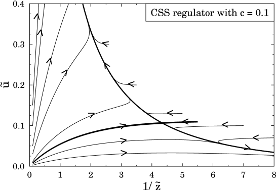
Figure 2: Phase diagram of the SG model for $d=1$ dimension is obtained by the usage of the CSS regulator (14) with $c=0.1$ including the wave function renormalization. Similar RG flow can be drawn for $1<d<2$. Arrows indicate the direction of the flow.

The two attractive IR fixed points ($\tilde{u}_{\star}=1.05$, $1/{\tilde{z}_{\star}}=0$ and $\tilde{u}_{\star}=0$, $1/{\tilde{z}_{\star}}=\infty$) indicate two phases. The coordinates of the non-trivial saddle point which separates the phases read as $\tilde{u}_{\star}=0.106$, $1/{\tilde{z}_{\star}}=4.34$. Using the normalized coupling $\bar{u}_{k}=k^{2}{\tilde{u}}/\bar{k}$ one obtains $\bar{u}_{\star}=0.47$ which is close to that of given by the power-law RG with $b=2$. Thus, the CSS RG provides us reliable results beyond LPA, too.

Although the detailed analysis of the regulator dependence of the above result is beyond the scope of the present work, let us briefly discuss the scheme-dependence of the RG study of the SG model for dimensions $d<1$ beyond LPA. Both for fractal dimensions $1<d<2$ and for $d=1$, the non-trivial saddle point appears in the RG flow of the SG model. However, there is an important difference between the two cases. In one-dimension as a consequence of the equivalence between quantum field theory and quantum mechanics a symmetry cannot be broken spontaneously due to the tunneling effect. Thus, for one-dimensional quantum field theoric models the (spontaneously) broken phase should vanish if their phase structure have been determined without using approximations. Therefore, the requirement of the absence of the broken phase in case of the non-approximated RG flow can be used to optimize the RG scheme-dependence of the approximated one [24]. The broken phase vanishes if the saddle point coincides with the non-trivial IR fixed point found at $\tilde{u}_{\star}=1.05$, $1/{\tilde{z}_{\star}}=0$. Thus, the distance between the saddle point and the non-trivial IR fixed point can be used to optimize the RG equations, i.e. the better the RG scheme is the closer the fixed points are [24]. We note that one has to use appropriately normalized couplings such as $\bar{u}_{k}=k^{2}{\tilde{u}}/\bar{k}$ and $\bar{z}_{k}\equiv(8\pi)\tilde{z}_{k}$. Then, the distance between the saddle point and the non-trivial IR fixed point should be minimized in order to obtain the optimal choice for the parameters of a given regulator function. In Ref. [24] this new type of optimization scenario was tested first for the power-law regulator and the known results were recovered. Then the optimization of the RG flow obtained by generalized CSS regulator function (15) was performed. It has importance since the generalized CSS regulator is a prototype regulator which recovers all major type of regulator functions in appropriate limits, thus, its optimization can produces us the best choice among the class of regulator functions. For example, it can be shown that by the fine tuning of the parameters of the CSS regulator it is possible to produce better results (smaller distance) then by the power-law type regulator [24].

6 Summary

In this work an example was given for a compactly supported smooth (CSS) regulator function. Similarly to the optimized (in a sense of [6, 10]) regulator it has a finite range, hence, the upper bound of the momentum integral of the functional RG equation is well-defined in numerical treatments and it is UV safe. Since the CSS regulator is a function of class $C^{\infty}$ its advantage is that it has derivatives of all orders in contrary to the optimized regulator which is continuous but not differentiable. This has important consequences on the applicability of the CSS regulator beyond the second order of the derivative expansion. It was also shown that in the limit $c\to 0$ the specified CSS regulator reduces to the optimized one (7), therefore, the smaller the parameter $c$ the closer the results obtained by the two regulators are. Moreover, it was also shown that the generalized form of the CSS regulator can be considered as a prototype regulator which reduces to all major type of regulator functions (exponential, power-law) in appropriate limits. Although, the usage of the CSS regulator at higher order of the derivative expansion requires considerable numerical efforts for small value of $c$ due to the sharp oscillatory peaks of higher derivates near $y=1$ but it is differentiable for $c\neq 0$, hence, it represents an approximation scheme to the optimized regulator in a sense of [10] at all orders of the derivative expansion. This was demonstrated by considering the critical behavior of the bosonized QED₂ in the local potential approximation. The CSS regulator has been tested beyond the local potential approximation in the framework of the sine-Gordon scalar theory for $d<2$ dimensions. A similar smoothing problem of nuclear physics was also discussed.

References

- [1] F. J. Wegner, A. Houghton, Phys. Rev. A. 8, 401 (1973).
- [2] J. Polchinski, Nucl. Phys B 231, 269 (1984).
- [3] C. Wetterich, Nucl. Phys. B 352, 529 (1991); ibid, Phys. Lett. B301, 90 (1993).
- [4] T. R. Morris, Int. J. Mod. Phys. A 9, 2411 (1994);
- [5] J. Alexandre, J. Polonyi, Annals Phys. 288, 37 (2001); J. Alexandre, J. Polonyi, K. Sailer, Phys. Lett. B 531, 316 (2002).
- [6] D. F. Litim, Phys. Lett. B 486, 92 (2000); ibid, Phys. Rev. D 64, 105007 (2001); ibid, JHEP 0111, 059 (2001).
- [7] D. F. Litim, Nucl.Phys. B 631, 128 (2002).
- [8] T. R. Morris, JHEP 0507, 027 (2005).
- [9] O. J. Rosten, Phys. Rept. 511, 177 (2012).
- [10] J. M. Pawlowski, Ann. Phys. 322, 2831 (2007);
- [11] Nándori, Phys. Rev. D 84, 065024 (2011).
- [12] I. Nándori, S. Nagy, K. Sailer, A. Trombettoni, Phys. Rev. D 80, 025008 (2009); ibid, JHEP 1009, 069 (2010).
- [13] L. Canet, B. Delamotte, D. Mouhanna and J. Vidal, Phys. Rev. D 67, 065004 (2003); ibid, Phys.Rev. B 68 064421 (2003); L. Canet, Phys.Rev. B 71 012418 (2005).
- [14] R. D. Ball, P. E. Haagensen, J. I. Latorre and E. Moreno, Phys. Lett. B 347, 80 (1995); D. F. Litim, Phys. Lett. B 393, 103 (1997); K. Aoki, K. Morikawa, W. Souma, J. Sumi and H. Terao, Prog. Theor. Phys. 99, 451 (1998); S.B. Liao, J. Polonyi, M. Strickland, Nucl. Phys. B 567, 493 (2000); J. I. Latorre and T. R. Morris, JHEP 0011, 004 (2000); F. Freire and D. F. Litim, Phys. Rev. D 64, 045014 (2001); D. F. Litim, JHEP 0507, 005 (2005); C. Bervillier, B. Boisseau, H. Giacomini, Nucl. Phys. B 789, 525 (2008); C. Bervillier, B. Boisseau, H. Giacomini, Nucl. Phys. B 801, 296 (2008); C. S. Fischer, A. Maas, J. M. Pawlowski, Ann. Phys. 324, 2408 (2009); S. Nagy, K. Sailer, arXiv:1012.3007 [hep-th]; S. Nagy, K. Sailer, Annals Phys. 326, 1839 (2011); S. Nagy, Nucl. Phys. B 864, 226 (2012); S. Nagy, Phys. Rev. D, 86, 085020 (2012).
- [15] S. Nagy, I. Nándori, J. Polonyi, K. Sailer, Phys. Rev. Lett. 102 241603 (2009).
- [16] O. Luscher, M. Reuter, Phys. Rev. D 66 025026 (2002); ibid Phys. Rev. D 65 025013 (2002).
- [17] J. Darai, R. Rácz, P. Salamon and R. G. Lovas, Phys. Rev. C 86, 014314 (2012).
- [18] P. Salamon, T. Vertse, Phys. Rev. C 77, 037302 (2008).
- [19] R. Rácz, P. Salamon and T. Vertse, Phys. Rev. C 84, 037602 (2011).
- [20] P. Salamon, A. T. Kruppa, T. Vertse, Phys. Rev. C 81, 064322 (2010).
- [21] P. Salamon, T. Vertse, L. Balkay, arXiv:1210.1721 [nucl-th].
- [22] T. M. Byrnes, P. Sriganesh, R. J. Bursill and C. J. Hamer, Phys. Rev. D 66, 013002 (2002).
- [23] I. Nándori, arXiv:1108.4643 [hep-th].
- [24] I. Nándori, I. G. Márián and V. Bacsó, arXiv:1303.4508 [hep-th].