Low-diffusivity scalar transport using a WENO scheme and dual meshing

Abstract

Interfacial mass transfer of low-diffusive substances in an unsteady flow environment is marked by a very thin boundary layer at the interface and other regions with steep concentration gradients. A numerical scheme capable of resolving accurately most details of this process is presented. In this scheme, the fifth-order accurate WENO method developed by Liu et al. [13] was implemented on a non-uniform staggered mesh to discretize the scalar convection while for the scalar diffusion a fourth-order accurate central discretization was employed. The discretization of the scalar convection-diffusion equation was combined with a fourth-order Navier-Stokes solver which solves the incompressible flow. A dual meshing strategy was employed, in which the scalar was solved on a finer mesh than the incompressible flow. The order of accuracy of the solver for one-dimensional scalar transport was tested on both stretched and uniform grids. Compared to the fifth-order WENO implementation of Jiang and Shu [10], the Liu et al. [13] method was found to be superior on very coarse meshes. The solver was further tested by performing a number of two-dimensional simulations. At first a grid refinement test was performed at zero viscosity with shear acting on an initially axisymmetric scalar distribution. A second refinement test was conducted for an unstably stratified flow with low diffusivity scalar transport. The unstable stratification led to buoyant convection which was modelled using a Boussinesq approximation with a linear relationship between flow temperature and density. The results show that for the method presented a relatively coarse mesh is sufficient to accurately describe the fluid flow, while the use of a refined dual mesh for the low-diffusive scalars is found to be beneficial in order to obtain a highly accurate resolution with negligible numerical diffusion.

1 Introduction

To accurately resolve low-diffusivity scalar transport problems special numerical schemes are necessary for the discretization of the convective term in order to avoid under- and/or overshoots of the scalar quantity. The first order upwind method, for example, could be used to effectively avoid such under- and/or overshoots but at the cost of introducing an excessive amount of numerical diffusion [5, 17]. Up to now, a number of DNS studies of gas transfer across the air-water interfaces have been carried out for shear driven and stirred vessels. Hasegawa and Kasagi [8] studied wind-shear driven mass transfer across the turbulent interface at a Schmidt number of $Sc=100$. They used a pseudo-spectral Fourier method for the spatial discretization in the horizontal directions, whereas the finite volume method is employed in the normal direction in which turbulent and molecular mass fluxes are evaluated at a cell surface with second-order accuracy. Handler et al. [6] used a pseudo spectral approach with Fourier expansions to carry out direct numerical simulations for the transport of a passive scalar at a shear-free boundary in fully developed channel flow. Similarly, Banerjee et al. also used a pseudo-spectral method to extensively study the mechanisms of turbulence and scalar exchange at the air-water interface in several publications (see [3, 2] and references therein). Schwertfirm and Manhart [15] also studied passive scalar transport in a turbulent channel flow for Schmidt numbers up to $Sc=49$. They used a similar approach as presented in the present work by solving the scalar on a finer grid than the velocity which was mapped by a conservative interpolation to the fine-grid. An explicit iterative finite-volume scheme of sixth-order accuracy was employed to calculate all convective and diffusive fluxes, while for the time-integration a third order Runge-Kutta method was used [16].

The pseudo-spectral methods used above have excellent error properties when the solution is relatively smooth. However, a main disadvantage of using spectral methods lies in the formation of non-physical oscillations near steep gradients that may regularly occur in the solution of a convection-diffusion problem when the diffusivity is extremely small. These Gibbs oscillations (under- and/or overshoots) [19] near steep gradients are not uncommon and can also be found when higher-order central finite-difference methods are used on a relatively coarse mesh to discretize the convection of a scalar with low diffusivity. This can be overcome by using weighted essentially non-oscillatory schemes (WENO) which have excellent shock capturing capabilities. Their non-oscillatory behaviour is advantageous in dealing with very steep gradients. In this paper, we present a numerical scheme developed specifically to resolve the details of the interfacial mass transfer of low-diffusive substances by adapting the weighted essentially non-oscillatory (WENO) by Liu et al. [13]. They are based on essentially non-oscillatory (ENO) schemes which were first published in the meanwhile classic paper of Harten et al. [7]. Liu et al. [13] introduced the idea of taking a convex combination of interpolation polynomials to construct a stencil using non-linear weights with a high order-of-accuracy in smooth regions while weighing out the non-smooth stencils in regions containing steep gradients or discontinuities. They studied WENO($2r-1$) schemes for different stencil sizes, i.e. $r=2$ (WENO3) and $r=3$ (WENO5).

In the meantime a large variety of WENO schemes has been developed. Many improvements were made by modifying the smoothness determination. For instance, Jiang and Shu [10] introduced a new smoothness indicator that is used to evaluate the non-linear weights. The size of the stencil has also been further increased by Balsara and Shu [1] extending it up to $r=6$ (WENO11). Henrick et al. [9] could show that the weights generated by the classical choice of smoothness indicators in [10] failed to recover the maximum order of the scheme at critical points of the solution where the first derivatives are zero. They developed the so called WENOM schemes where a mapping procedure is introduced to keep the weights of the stencils as close as possible to the optimal weights. The resulting (mapped) WENOM scheme of Henrick et al. [9] presented more accurate results close to discontinuities. Even more recently, Borges et al. [4] achieved the same results as mapped WENO schemes without mapping but by improving the accuracy of the classical WENO5 scheme by devising a new smoothness indicator and non-linear weights using the whole 5-points stencil and not the classical smoothness indicator of Jiang and Shu [10] which uses a composition of three 3-points stencils. The schemes of Borges et al. [4] are known as WENO-Z schemes. Of all the schemes discussed above the classical WENO5 scheme is used most widely [9, 14, 12]. In our simulations we do not expect any discontinuities in the scalar field so that the classical WENO5 scheme of Liu et al. [13] is a good choice to accurately resolve low-diffusive scalar transport which may lead to steep concentration gradients.

An example of application is given for the 2D case of buoyant-convectively driven mass transfer with a Prandtl number of $Pr=6$ and a Schmidt number of $Sc=500$. One typical process in nature of such a case is the absorption of oxygen into lakes during night time. This process is controlled by the low diffusivity of the dissolved gas in the water and the convective instability triggered by the density difference between the cold water at the top surface and the warm water in the bulk. The convective-instability enhances the gas transfer into the water body significantly compared with the static condition with only diffusive gas transfer. This low diffusive process results in a very thin concentration boundary layer that is found at the water surface. Experimental measurements near the surface (such as the mass flux) are very difficult. There is a need to fully resolve the near surface mechanisms in order to understand the physical mechanism.

Below, the capability of the newly developed code to accurately resolve low-diffusivity scalar transport problems will be illustrated. First the full set of 2D equations to be solved and the formulation of the numerical schemes used in Section 2 are presented. Section 3 covers 1D numerical experiments that were performed to determine the accuracy of the applied schemes on uniform and stretched meshes for both purely convective and purely diffusive scalar transport. The numerical schemes were further tested by performing a number of 2D-simulations. The first 2D application case, presented in Section 4, deals with a zero-viscosity steady shear flow acting on an initially axisymmetric scalar distribution. In the last section the solver was tested for the 2D case of low-diffusivity scalar transport in buoyancy driven flow.

2 Formulation of Numerical Method

The full set of the 2D governing equations to be solved in order to address/simulate the low-diffusivity scalar transport problem are first presented in this section followed by the formulation of the numerical schemes used. For the scalar transport the two-dimensional convection diffusion equation of the scalar $\varphi=\varphi(x,z,t)$ in conservative form reads

$$\frac{\partial\varphi}{\partial t}+\frac{\partial u\varphi}{\partial x}+\frac{\partial w\varphi}{\partial z}=D\left(\frac{\partial^{2}\varphi}{\partial x^{2}}+\frac{\partial^{2}\varphi}{\partial z^{2}}\right),$$ (1)

where $x$ and $z$ are the horizontal and vertical directions, respectively, $u$ and $w$ are the velocities in the $x$ and $z$ directions, $D$ is the molecular diffusion coefficient of the dissolved substance and $t$ denotes time.

For the flow-field the incompressible Navier-Stokes equation is solved. The continuity equation for two-dimensional incompressible flow reads,

$$\frac{\partial u}{\partial x}+\frac{\partial w}{\partial z}=0,$$ (2)

and the momentum equations are given by

$$\frac{\partial u}{\partial t} = -\frac{\partial p}{\partial x}+a$$ (3)

$$\frac{\partial w}{\partial t} = -\frac{\partial p}{\partial z}+c$$ (4)

where $p$ is pressure and $a$ and $c$ represent the sum of the convective and diffusive terms

$$a = -\frac{\partial u^{2}}{\partial x}-\frac{\partial uw}{\partial z}+\frac{1}{Re}\left\{\frac{\partial^{2}u}{\partial x^{2}}+\frac{\partial^{2}u}{\partial z^{2}}\right\}$$ (5)

$$c = -\frac{\partial w^{2}}{\partial z}-\frac{\partial uw}{\partial x}+\frac{1}{Re}\left\{\frac{\partial^{2}w}{\partial x^{2}}+\frac{\partial^{2}w}{\partial z^{2}}\right\}$$ (6)

where $Re$ is the Reynolds number.

2.1 Discretization of the convection-diffusion equation of the scalar $\varphi$

In this section we outline the discretization of the transport equation for the scalar $\varphi$ as given in equation (1). The diffusive term on the right of (1) is discretized using a fourth-order accurate central scheme, while the convective term is discretized using variants of the fifth-order WENO schemes developed by Liu et al. [13] and Jiang and Shu [10]. The WENO schemes use an approximation of the scalar fluxes at the cell interface by employing interpolation schemes. The reconstruction procedure produces a high order accurate approximation of the solution from the calculated cell averages. Below the implemented scheme is detailed only in one dimension. Generalization to higher dimensions is straightforward.

When ignoring the diffusive term, the one dimensional variant of (1) can be rewritten as

$$\frac{\partial\varphi}{\partial t}=-\frac{\partial u\varphi}{\partial x}$$ (7)

where $u$ is the velocity in the $x$-direction. As we employ a staggered mesh, for the volume centred around $x=x_{i}$, the convective fluxes $R_{i}^{+}$ and $R_{i}^{-}$ are defined by

$$R_{i}^{+} = \frac{a_{0}}{a_{0}+a_{1}+a_{2}}P_{i-1}(x_{i+\frac{1}{2}})+\frac{a_{1}}{a_{0}+a_{1}+a_{2}}P_{i}(x_{i+\frac{1}{2}})+\frac{a_{2}}{a_{0}+a_{1}+a_{2}}P_{i+1}(x_{i+\frac{1}{2}})$$ (8)

and

$$R_{i}^{-} = \frac{a_{0}}{a_{0}+a_{1}+a_{2}}P_{i-1}(x_{i-\frac{1}{2}})+\frac{a_{1}}{a_{0}+a_{1}+a_{2}}P_{i}(x_{i-\frac{1}{2}})+\frac{a_{2}}{a_{0}+a_{1}+a_{2}}P_{i+1}(x_{i-\frac{1}{2}})$$ (9)

where $a_{0},a_{1},a_{2}$ are coefficients and $P$ the Lagrange interpolations polynomials defined in (16). In the implementation of Liu et al. [13], for $R_{i}^{+}$ the weights for the convex combination of the quadratic Lagrange interpolation polynomials are given by,

$$a_{0}=\frac{1}{12(\varepsilon+IS_{i})^{3}},\;\;a_{1}=\frac{1}{2(\varepsilon+IS_{i+1})^{3}},\;\;a_{2}=\frac{1}{4(\varepsilon+IS_{i+2})^{3}},$$ (10)

while for $R_{i}^{-}$ the weights are given by

$$a_{0}=\frac{1}{4(\varepsilon+IS_{i})^{3}},\;\;a_{1}=\frac{1}{2(\varepsilon+IS_{i+1})^{3}},\;\;a_{2}=\frac{1}{12(\varepsilon+IS_{i+2})^{3}},$$ (11)

where $\varepsilon=10^{-6}$ and the smoothness indicator $IS_{i}$ is defined by

$$IS_{i}=\frac{1}{2}((\varphi_{i-1}-\varphi_{i-2})^{2}+(\varphi_{i}-\varphi_{i-1})^{2})+(\varphi_{i}-2\varphi_{i-1}+\varphi_{i-2})^{2}.$$ (12)

The original calculation of the weights $a_{0}$, $a_{1}$ and $a_{2}$ as presented above is compared to an alternative developed by Jiang and Shu [10], in which the weights for $R_{i}^{+}$ are given by

$$a_{0}=\frac{1}{10(\varepsilon+IS_{0})^{r}},\;\;a_{1}=\frac{6}{10(\varepsilon+IS_{1})^{r}},\;\;a_{2}=\frac{3}{10(\varepsilon+IS_{2})^{r}},$$ (13)

while for $R_{i}^{-}$ the weights are given by

$$a_{0}=\frac{3}{10(\varepsilon+IS_{0})^{r}},\;\;a_{1}=\frac{6}{10(\varepsilon+IS_{1})^{r}},\;\;a_{2}=\frac{1}{10(\varepsilon+IS_{2})^{r}},$$ (14)

with the smoothness indicators $IS_{i}$ defined by

$$IS_{0} = \frac{13}{12}(\varphi_{i-2}-2\varphi_{i-1}+\varphi_{i})^{2}+\frac{1}{4}(\varphi_{i-2}-4\varphi_{i-1}+3\varphi_{i})^{2}$$

$$IS_{1} = \frac{13}{12}(\varphi_{i-1}-2\varphi_{i}+\varphi_{i+1})^{2}+\frac{1}{4}(\varphi_{i-1}-\varphi_{i+1})^{2}$$

$$IS_{2} = \frac{13}{12}(\varphi_{i}-2\varphi_{i+1}+\varphi_{i+2})^{2}+\frac{1}{4}(3\varphi_{i}-4\varphi_{i+1}+\varphi_{i+2})^{2}.$$ (15)

Note that in the 1D tests presented below a power of $r=3$ in (13) and (14) was used. The upstream central method can be obtained from both the Liu et al. [13] and Jiang and Shu [10] implementations of the weights by setting all smoothness indicators $IS$ in (10), (11) and (13), (14) to zero.

The modified quadratic Lagrange interpolations $P_{i}(x)$ in equations (8) and (9) read

$$P_{i}(x)= \frac{(x-x_{i})(x-x_{i+1})}{(x_{i-1}-x_{i})(x_{i-1}-x_{i+1})}\varphi_{i-1}+\frac{(x-x_{i-1})(x-x_{i+1})}{(x_{i}-x_{i-1})(x_{i}-x_{i+1})}\varphi_{i}+\frac{(x-x_{i-1})(x-x_{i})}{(x_{i+1}-x_{i-1})(x_{i+1}-x_{i})}\varphi_{i+1}$$ (16)

$$-\frac{(x_{i}-x_{i-1})\varphi_{i+1}-(x_{i+1}-x_{i-1})\varphi_{i}+(x_{i+1}-x_{i})\varphi_{i-1}}{12(x_{i+1}-x_{i})}$$

High-order polynomial interpolations to the midpoints $x_{i+\frac{1}{2}}$ are computed using known grid values of the scalar $\varphi$. The scheme uses a 5-points stencil which is divided into three 3-points stencils as shown in Fig. 1.

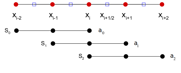
Figure 1: Schematic illustration of the weighted 5 point convex combination composed of three 3-points stencils $S_{0},S_{1},S_{2}$ and their respective weights $a_{0},a_{1},a_{2}$ used in the classical WENO5 scheme. [18].

These are interpolations of the scalar to the faces of the volume combined with a smoothing term at the right. Using the above, depending on the signs of $u_{i-\frac{1}{2}}$ and $u_{i+\frac{1}{2}}$, we have four possible ways to calculate the discretization of the convective terms $L_{i}(\varphi)~{}=~{}\left(-u\frac{\partial\varphi}{\partial x}\right)|_{x_{i}}$ in $x_{i}$:

$$u_{i+\frac{1}{2}}>0,u_{i-\frac{1}{2}}>0:L_{i}(\varphi) = -\frac{u_{i+\frac{1}{2}}R^{+}_{i}-u_{i-\frac{1}{2}}R^{+}_{i-1}}{x_{i+\frac{1}{2}}-x_{i-\frac{1}{2}}}$$

$$u_{i+\frac{1}{2}}>0,u_{i-\frac{1}{2}}<0:L_{i}(\varphi) = -\frac{u_{i+\frac{1}{2}}R^{+}_{i}-u_{i-\frac{1}{2}}R^{-}_{i}}{x_{i+\frac{1}{2}}-x_{i-\frac{1}{2}}}$$

$$u_{i+\frac{1}{2}}<0,u_{i-\frac{1}{2}}>0:L_{i}(\varphi) = -\frac{u_{i+\frac{1}{2}}R^{-}_{i+1}-u_{i-\frac{1}{2}}R^{+}_{i-1}}{x_{i+\frac{1}{2}}-x_{i-\frac{1}{2}}}$$

$$u_{i+\frac{1}{2}}<0,u_{i-\frac{1}{2}}<0:L_{i}(\varphi) = -\frac{u_{i+\frac{1}{2}}R^{-}_{i+1}-u_{i-\frac{1}{2}}R^{-}_{i}}{x_{i+\frac{1}{2}}-x_{i-\frac{1}{2}}}$$

By examining the equations above it can be seen that at each interface $x_{i+\frac{1}{2}}$ of 2 neighbouring cells the scalar flux (either $u_{i+\frac{1}{2}}R^{+}_{i}$ or $u_{i+\frac{1}{2}}R^{-}_{i+1}$) is uniquely determined, which ensures that any scalar quantity that leaves the volume centred around $x_{i}$ through this interface will enter the volume centred around $x_{i+1}$. Upwind information is incorporated by the way in which the scalar at each cell interface is interpolated. For instance, the interpolation stencil for $R^{+}_{i}$ (8) - which is employed when $u_{i+\frac{1}{2}}>0$ and consists of five points with $x=x_{i}$ in the middle - is used to calculate the scalar at the location $x=x_{i+\frac{1}{2}}$ which is located upstream (upwind) of $x=x_{i}$. A similar argument holds for the calculation of $R^{-}_{i}$ (9). Hence, both stencils are non-symmetric and use more information from the upwind direction than from the downwind direction. Based on this bias, the method discussed above can be classified as an upwind method.
With the methods described here a fifth-order accuracy can be achieved. Note that the weights given to the interpolating polynomials $a_{0},a_{1},a_{2}$ depend on the local smoothness of the solution. Interpolation polynomials defined in regions where the solution is smooth are given higher weights than those in regions near discontinuities (shocks) or steep gradients (like the gas concentration near the interface in our application case presented in Section 5).

The diffusive term on the right hand side of (1) is discretized using a fourth-order central finite difference method for the second derivative such as,

$$\frac{\partial^{2}\varphi}{\partial x^{2}}\approx\frac{-\varphi_{i+2,k}+16\varphi_{i+1,k}-30\varphi_{i,k}+16\varphi_{i-1,k}-\varphi_{i-2,k}}{12(\delta x_{i})^{2}}$$ (17)

and

$$\frac{\partial^{2}\varphi}{\partial z^{2}}\approx\frac{-\varphi_{i,k+2}+16\varphi_{i,k+1}-30\varphi_{i,k}+16\varphi_{i,k-1}-\varphi_{i,k-2}}{12(\delta z_{k})^{2}}$$ (18)

where $\delta x_{i}=x_{i+\frac{1}{2}}-x_{i-\frac{1}{2}}$ and $\delta z_{k}=z_{k+\frac{1}{2}}-z_{k-\frac{1}{2}}$, respectively. On a stretched mesh the actual discretization coefficients are obtained from the above equations using Lagrange interpolations to a seven-point numerical stencil. The time integration of the convection-diffusion equation is implemented using a third order Runge-Kutta method (RK3) developed by Shu and Osher [18] that reads,

$$\varphi_{i}^{(1)} = \varphi_{i}^{n}+\Delta tL_{i}(\varphi_{i}^{n})$$

$$\varphi_{i}^{(2)} = \frac{3}{4}\varphi_{i}^{n}+\frac{1}{4}\varphi_{i}^{(1)}+\frac{1}{4}\Delta tL_{i}(\varphi_{i}^{(1)})$$

$$\varphi_{i}^{(n+1)} = \frac{1}{3}\varphi_{i}^{n}+\frac{2}{3}\varphi_{i}^{(2)}+\frac{2}{3}\Delta tL_{i}(\varphi_{i}^{(2)})$$ (19)

2.2 Flow Solver

This section outlines the numerical method of the flow solver used in the two-dimensional simulations presented in Sections 4 and 5. The velocity field is solved by a finite-difference discretization of the convective terms using a fourth-order unconditionally kinetic energy conserving method combined with a fourth-order accurate central method for the diffusive terms [20]. The 2D incompressible Navier-Stokes equation is discretized on a non-uniform, staggered mesh in combination with a second-order accurate Adams-Bashforth time integration. The continuity equation (2) for the two-dimensional incompressible flow in discretized form on a mesh as shown in Fig. 2a

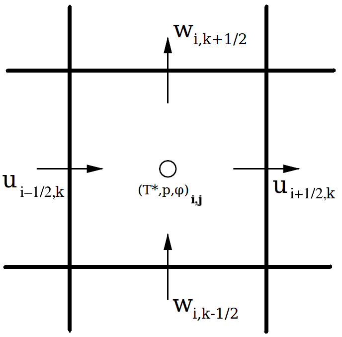
(a) Variables on a staggered mesh

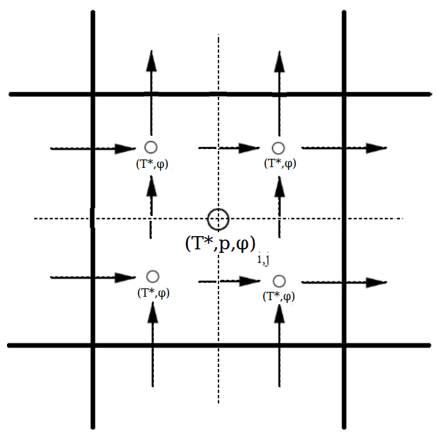
(b) Dual sub-mesh refined by factor R = 2

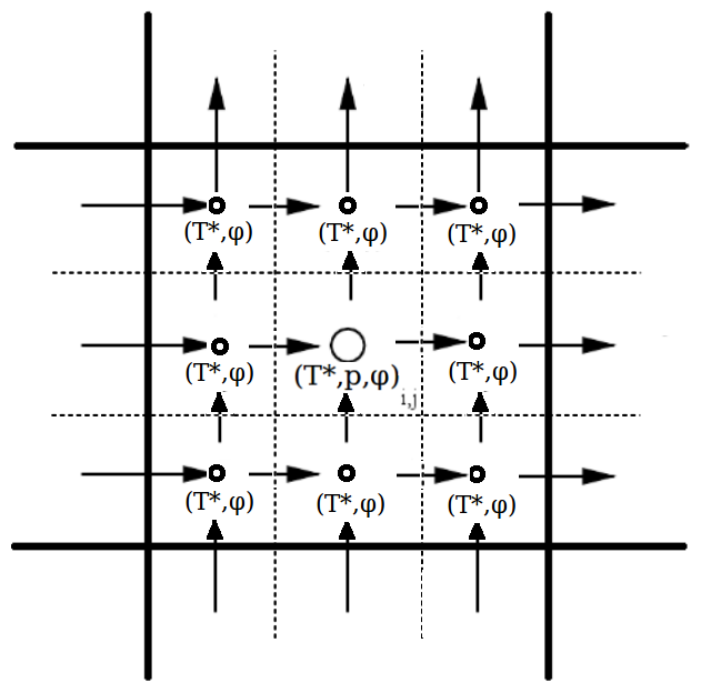
(c) Dual sub-mesh refined by factor R = 3

Figure 2: Variables on the new dual mesh. The flow field is solved on the outer coarse mesh, whilst the scalar is computed on a refined subgrid. For the transport of the scalar the velocities are interpolated onto the midpoints of the subgrid

reads

$$\frac{u_{i+\frac{1}{2},k}^{n+1}-u_{i-\frac{1}{2},k}^{n+1}}{x_{i+\frac{1}{2}}-x_{i-\frac{1}{2}}}+\frac{w_{i,k+\frac{1}{2}}^{n+1}-w_{i,k-\frac{1}{2}}^{n+1}}{z_{k+\frac{1}{2}}-z_{k-\frac{1}{2}}}=0$$ (20)

When substituting the momentum equation into the continuity equation a Poisson equation for the pressure is obtained. The Poisson equation is iteratively solved using the conjugate gradient method with a diagonal preconditioning. From the obtained pressure field the new velocity field can be calculated by rearranging the discretized equations of (3) and (4),

$$u^{n+1}_{i+\frac{1}{2},k}=u^{n}_{i+\frac{1}{2},k}+\varDelta t\left\{-\frac{p_{i+1,k}^{n+1}-p_{i,k}^{n+1}}{x_{i+1}-x_{i}}+a^{n}_{i+\frac{1}{2},k}\right\}$$ (21)

$$w^{n+1}_{i,k+\frac{1}{2}}=w^{n}_{i,k+\frac{1}{2}}+\varDelta t\left\{-\frac{p_{i,k+1}^{n}-p_{i,k}^{n+1}}{z_{k+1}-z_{k}}+c^{n}_{i,k+\frac{1}{2}}\right\}.$$ (22)

Fig. 2a shows the location of variables on a staggered mesh. To achieve kinetic energy conservation interpolations are required to evaluate the convective term. For instance at $(x_{i+\frac{1}{2}},z_{k})$ only the $u$-velocity component is available at that location, while the $w$-velocity is only available at $(x_{i},z_{k+\frac{1}{2}})$. Hence an interpolation of $w$ to the position where $u$ is defined gives $\overline{w}_{i+\frac{1}{2},k}$. An equivalent procedure for the $z$-momentum where $u$ needs to be interpolated where $w$ is defined gives $\overline{u}_{i,k+\frac{1}{2}}$. This yields to the discretization of the convective terms by a fourth-order central discretization,

$$C_{x}(u,\overline{w})_{i+\frac{1}{2},k}= -\frac{1}{2}\left[\frac{1}{-x_{i+\frac{5}{2}}+8x_{i+\frac{3}{2}}-8x_{i-\frac{1}{2}}+x_{i-\frac{3}{2}}}\Big{\{}-u_{i+\frac{5}{2},k}(u_{i+\frac{1}{2},k}+u_{i+\frac{5}{2},k})+8u_{i+\frac{3}{2},k}(u_{i+\frac{1}{2},k}+u_{i+\frac{3}{2},k})\right.$$

$$\left.-8u_{i-\frac{1}{2},k}(u_{i+\frac{1}{2},k}+u_{i-\frac{1}{2},k})+u_{i-\frac{3}{2},k}(u_{i+\frac{1}{2},k}+u_{i-\frac{3}{2},k})\Big{\}}+\frac{1}{-z_{k+2}+8z_{k+1}-8z_{k-1}+z_{k-2}}\right.$$

$$\left.\times\Big{\{}-u_{i+\frac{1}{2},k+2}(\overline{w}_{i+\frac{1}{2},k}+\overline{w}_{i+\frac{1}{2},k+2})+8u_{i+\frac{1}{2},k+1}(\overline{w}_{i+\frac{1}{2},k}+\overline{w}_{i+\frac{1}{2},k+1})-8u_{i+\frac{1}{2},k-1}(\overline{w}_{i+\frac{1}{2},k}+\overline{w}_{i+\frac{1}{2},k-1})\right.$$

$$\left.+u_{i+\frac{1}{2},k-2}(\overline{w}_{i+\frac{1}{2},k}+\overline{w}_{i+\frac{1}{2},k-2})\Big{\}}\right]$$ (23)

The convective terms in the $z$ -direction are discretized in a similar manner. The diffusive terms are discretized using the fourth-order accurate central discretization scheme ((17) and (18)) in which the coefficients of the seven point stencil employed for the discretization on a non-uniform mesh are determined using Lagrange interpolations.

2.3 Dual Mesh Approach

Because the diffusivity of the scalars of interest is up to three orders of magnitude smaller than that of the momentum, the resolution requirements for the flow field is less stringent as shown by the mesh refinement test in Section 5.2. Thus, to save computing time a dual mesh approach is used as illustrated in Fig. 2. The velocity is solved on a coarser base mesh (Fig. 2a), while the scalar is defined on the finer subgrid (Fig. 2b and 2c) so that the required computational resources are significantly reduced.

To calculate the convective transport of the scalar, the velocities are interpolated onto a subgrid using a fourth-order Lagrange interpolation. When employing a subgrid refinement by a factor of $R=2$ (Fig. 2b) an interpolation is required for each subcell as the velocity location and the scalar locations do not coincide with their counter parts on the base mesh. In contrast, Fig. 2c shows that in the case of a subgrid refinement by a factor $R=3$ some velocities and the central subcells for a scalar are defined at the same locations.

2.4 Implementation of Boundary Conditions

Dirichlet and Neumann boundary conditions are implemented by extrapolating the values obtained at the latest time step to ghost cells outside of the computational domain. This has the advantage that there is no need to change the numerical stencils near boundaries. Suppose the quantity $q$ is defined on an $N$-point mesh and we want to implement a Dirichlet (odd) boundary condition $q_{N}=Q$. By using the known values $q_{\frac{1}{2}},q_{\frac{3}{2}},\ldots,q_{N-\frac{1}{2}}$, the values $q_{N+i-\frac{1}{2}}$ are determined by using the formula

$$q_{N+i-\frac{1}{2}} = 2\,Q-q_{N-i+\frac{1}{2}}\;\;\mbox{for}\;\;i=1,\ldots,3.$$ (24)

To implement the Neumann (even) boundary condition at $i=0$, we use the formula

$$q_{-i+\frac{1}{2}} = q_{i-\frac{1}{2}}\;\;\mbox{for}\;\;i=1,\ldots,3.$$ (25)

The free-slip condition for the velocity is implemented by using a Neumann boundary condition (25) of the velocity component that is parallel to the boundary and a Dirichlet boundary condition (24) for the component that is orthogonal to the boundary (using the value zero at the boundary itself).

3 1D Numerical Experiments

In this section we apply the WENO-scheme for different test problems with the purpose of predicting the accuracy of the method on uniform and stretched meshes, respectively. As the problem is a convection-diffusion problem the numerical scheme was tested for both, scalar transport by convection only and by diffusion only.

3.1 Scalar transport by convection on a uniform grid

By using the modified quadratic Lagrange interpolations for reconstruction (16) we expect to achieve a fifth-order accuracy for the convective scalar transport on uniform meshes. In both of the following cases (uniform and non-uniform meshes), we use the previously described WENO schemes for spatial discretization and the $3^{rd}$-order Runge-Kutta-scheme for time integration of the one-dimensional convection equation. Because we want to predict the numerical error in the WENO scheme, physical diffusion will be neglected. If $\varphi(x_{i},t)$ and $\varphi_{exact}$ are the numerical and the exact solutions, respectively at $(x_{i},t)$, the $\L_{1}$ discretization error is given by

$$\L_{1}=\frac{1}{N}\displaystyle\sum_{i=1}^{N}\mid\varphi(x_{i},t)-\varphi_{exact}\mid,$$ (26)

where $N$ describes the number of nodes in the domain, $t$ the time, $i$ the node number.

At first the WENO schemes are tested in a one-dimensional (1D) domain using uniform meshes. Therefore, the 1D scalar convection equation,

$$\frac{\partial\varphi}{\partial t}+\frac{\partial\varphi}{\partial x}=0,$$ (27)

was discretized on $0\leq x\leq 2$ using periodic boundary conditions at $x=0$ and $x=2$. The scalar distribution was initialized by a sine wave function $\varphi(x,0)=\varphi_{0}(x)=\sin{(\pi x)}$.

In the calculations an extremely small CFL-number was used so that the time-step would be small enough to ensure that the third-order temporal behaviour of the Runge-Kutta scheme would not affect the rate of convergence of the WENO schemes.

Table 1

WENO-Liu et al. [13]			WENO-Jiang and Shu [10]			Upstream Central
$N$	$\L_{1}$-error	order	$N$	$\L_{1}$-error	order	$N$	$\L_{1}$-error	order
10	1.17 E-02	-	10	2.11 E-02	-	10	3.11 E-03	-
20	2.47 E-03	2.24	20	1.10 E-03	4.27	20	1.01 E-04	4.95
40	3.30 E-04	2.90	40	3.26 E-05	5.07	40	3.18 E-06	4.99
80	2.53 E-05	3.70	80	9.98 E-07	5.03	80	9.99 E-08	4.99
160	1.57 E-06	4.01	160	3.12 E-08	5.00	160	3.15 E-09	4.99
320	6.13 E-08	4.68	320	9.76 E-10	5.00	320	1.03 E-10	4.94
640	1.04 E-09	5.89	640	3.13 E-11	4.96	640	4.26 E-12	4.59

Table 1: Absolute error and order of convergence on uniform meshes with $\varepsilon=10^{-6}$.

gives the $\L_{1}$ error after running the simulation during one time-unit as well as the resulting order of accuracy. The WENO5 implementation of Liu et al. [13] was compared to the alternative WENO5 scheme developed by Jiang and Shu [10] and the upstream central method that is obtained by selecting the smoothness indicators $IS_{i}=0$ in either of the WENO schemes. Starting from $N=10$ nodes the $\L_{1}$ error is decreasing when increasing the number of nodes to 20, 40,…, 640. As previously found by Jiang and Shu [10], the implementation of Liu et al. [13] shows a smaller error than the scheme of Jiang and Shu [10] on the coarse 10-point mesh while on finer meshes the Jiang and Shu [10] implementation is superior.

Furthermore, the scheme of Jiang and Shu [10] as well as the upstream central scheme show a fifth-order behaviour, while the original scheme of Liu et al. [13] would need an even finer mesh to exhibit this behaviour. With the mesh sizes shown in the table, we would need to increase $\varepsilon$ significantly (even up to a value of $\varepsilon=1$) to achieve higher order. The choice of the small $\varepsilon=10^{-6}$ was necessary for the present application in order to resolve very steep gradients. To test whether the Liu et al. [13] scheme has the potential to exhibit a fifth-order behaviour, an additional test had been carried out in which $\varepsilon$ was increased to $\varepsilon=1$ (Table 2).

WENO-Liu et al. [13]
$N$	$\L_{1}$-error	order
10	3.46E-03	-
20	1.76E-04	4.30E+00
40	2.83E-06	5.96E+00
80	9.44E-08	4.91E+00
160	3.11E-09	4.92E+00
320	1.02E-10	4.93E+00
640	4.26E-12	4.59E+00

Table 2: Absolute error and order of convergence on uniform meshes with $\varepsilon=1$.

As can be seen in Table 2 for $\varepsilon=1$, indeed a fifth order behaviour for the original scheme was observed for $N\geq 80$ grid points. The slight decrease in order of convergence for $N=640$ points is possibly caused by machine-accuracy limitations affecting the calculations.

In practical calculations the mesh will be relatively coarse so that the original WENO implementation of Liu et al. [13], which has a good accuracy on coarse meshes, would be a good choice. Though the fifth-order upstream central method is shown to be even more accurate on coarse meshes, it is not the method of choice as the absence of a mechanism to deal with steep gradients could result in the appearance of wiggles as will be briefly discussed in Section 5.1.

3.2 Scalar transport by convection on non-uniform meshes

Using the modified Lagrange interpolations the WENO-scheme has been applied on non-uniform meshes on which the node distribution is given by:

$$x(i) = \left[1-\frac{\mathrm{tanh}(x_{\phi})}{\mathrm{tanh}(x_{1})}\right]x(0)+\left[\frac{\mathrm{tanh}(x_{\phi})}{\mathrm{tanh}(x_{1})}\right]x(n_{x})$$ (28)

for $i=1,...,n_{x}-1$, with

$$x_{\phi} = \delta/2\frac{i}{n_{x}}$$

$$x_{1} = \delta/2.$$

The procedure for the stretching is controlled by the parameter $\delta$. The $N$-point mesh distribution is so that $x(0)=0$ and $x(n_{x})=1$ where $n_{x}=N/2$. The resulting mesh is subsequently mirrored about $x=1$ to obtain the grid points between $x(n_{x})=1$ and $x(N)=2$.

The results of the tests using $\delta=1.0$ and $3.0$ is presented in Table 3.

$\delta=1.0$			$\delta=3.0$
$N$	$\L_{1}$-error	$\L_{1}$-order	$N$	$\L_{1}$-error	$\L_{1}$-order
10	1.20E-02	-	10	3.58E-02	-
20	2.41E-03	2.32E+00	20	6.28E-03	2.51E+00
40	3.91E-04	2.63E+00	40	1.60E-03	1.98E+00
80	6.27E-05	2.64E+00	80	3.77E-04	2.08E+00
160	1.41E-05	2.15E+00	160	9.26E-05	2.03E+00
320	3.45E-06	2.03E+00	320	2.31E-05	2.00E+00
640	8.62E-07	2.00E+00	640	5.77E-06	2.00E+00

Table 3: Absolute error and order of convergence on non-uniform meshes with $\varepsilon=10^{-6}$.

The absolute errors, as expected, are smaller for the mesh with reduced stretching. Compared to uniform meshes it can be seen that the order of accuracy decreases to approximately 2.

3.3 Scalar transport: pure diffusion

In this section we apply the fourth-order accurate central discretization (17) for the solution of scalar diffusion. In the one-dimensional case, concentration gradients in the $y$- and $z$ -directions are zero, and we have the one-dimensional diffusion equation for a scalar $\varphi(x,t)$

$$\frac{\partial\varphi}{\partial t}=D\frac{\partial^{2}\varphi}{\partial x^{2}}.$$ (29)

For the test a one-dimensional domain was chosen with $0\leq x\leq 5L$. A mesh with $N$ grid points was defined with a refinement near the surface where the concentration boundary layer will form. At $x=0$ the boundary condition $\varphi(0,t)=1$ was imposed. The analytical solution for this boundary value problem is given by

$$\varphi(x,t)=1-\mathrm{erf}\left(\frac{x}{\sqrt{4Dt}}\right).$$ (30)

The initial condition for the test was given by the analytical solution as defined in (30) at $t$=10 seconds. In the case of diffusive gas transfer into a liquid $D=\frac{1}{ReSc}$ and for the transfer of oxygen into water we have a Schmidt number of $Sc=500$ and a Reynolds number of $Re=100$, which is based on a characteristic length scale of $L=1$ cm and a characteristic velocity of $u=1$ cm/s. The latter gives us a characteristic time scale of $\theta=L/U=1$ second.

The absolute errors and order of accuracy for the pure diffusion scalar transport on non-uniform meshes were tested for $N=10$ to $640$. The results after 1 time-unit are shown in Table 4.

$\delta=3.0$			$\delta=4.5$
$N$	$\L_{1}$-error	$\L_{1}$-order	$N$	$\L_{1}$-error	$\L_{1}$-order
10	1.47E-04	-	10	1.27E-03	-
20	2.22E-04	-5.95E-01	20	3.26E-04	1.96E+00
40	2.45E-04	-1.41E-01	40	2.53E-05	3.69E+00
80	2.11E-05	3.54E+00	80	1.50E-06	4.07E+00
160	1.73E-06	3.61E+00	160	1.00E-07	3.91E+00
320	1.12E-07	3.95E+00	320	6.72E-09	3.90E+00
640	7.19E-09	3.96E+00	640	4.37E-10	3.94E+00

Table 4: Absolute error and order of convergence on non-uniform meshes for pure diffusion case.

The absolute errors in the numerical results are very small, illustrating very good agreement with the analytical solution. A fourth order accuracy is achieved even with increased stretching.

All 1D numerical tests described above (Sections 3.1 to 3.3) illustrate the advantageous behaviour of the chosen combination of a WENO-scheme with a fourth-order discretization of the diffusive terms which resulted in a low numerical diffusion and small absolute errors for both modes of transport, pure convection and pure diffusion, respectively.

4 Two dimensional sheared scalar distribution

To further test the robustness of the numerical scheme, we perform mesh sensitivity tests in 2D for two application cases, namely for sheared scalar distribution and low-diffusivity scalar transport in buoyancy driven flow. The first problem deals with a smooth scalar distribution without scalar diffusion being sheared by a zero viscosity flow as shown in Figure 3.

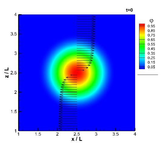
(a) $t=$ 0 s

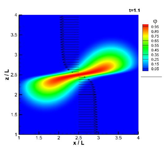
(b) $t=$ 1.1 s

Figure 3: A detail of the sheared scalar distribution. a) at $t$=0 second and b) at $t$=1.1 seconds.

After $1$ time-unit the flow is reversed with the aim to obtain the initial distribution of the scalar back so that the distribution at $t=0$ should be the same as at $t=2$.

The simulation was run on a $5L\times 5L$ domain using periodic boundary conditions in the horizonal direction and free-slip boundary conditions for the velocity combined with zero-flux boundary conditions (25) for the scalar along the upper and lower boundaries. At $t=0$, the scalar field was initialised by

$$\varphi_{i,k}=0.5\left(1+\cos(\pi\sqrt{(x_{i}-2.5)^{2}+(z_{k}-2.5)^{2}}\;)\right),$$ (31)

while the flow field was initialised using

$$u_{i+\frac{1}{2},k}=2\;\frac{\mathrm{atan}(10(z_{k}-2.5))}{\pi}.$$ (32)

At $t=1$ second the flow field was reversed, so that

$$u_{i+\frac{1}{2},k}=-2\;\frac{\mathrm{atan}(10(z_{k}-2.5))}{\pi}.$$ (33)

After $t=2$ seconds of simulation the error is determined by comparing the initial to the calculated scalar distribution. As can be seen in Table 5, a grid refinement study was carried out by performing simulations on a sequence of uniform meshes with $80\times 80$ up to $640\times 640$ points. With increasing number of grid points the order of accuracy was found to increase significantly from about 2 to 4.

$n_{x}\times n_{z}$	$\L_{1}$-error	$\L_{1}$-order
$40\times 40$	1.34E-03	-
$80\times 80$	3.51E-04	1.93E+00
$160\times 160$	7.30E-05	2.26E+00
$320\times 320$	9.33E-06	2.97E+00
$640\times 640$	5.92E-07	3.98E+00

Table 5: Absolute error and order of convergence resulting from the 2D sheared scalar distribution test on uniform meshes using the WENO scheme of Liu et al. [13] with $\varepsilon=10^{-6}$.

5 Two-dimensional low-diffusivity scalar transport in buoyancy driven flow

The second 2D application case considers the problem of low-diffusivity (high Schmidt number) mass transfer in buoyant-convectively driven flow. An example in nature is the oxygen absorption through the air-water interface in lakes at nighttime when the lakes’ surface is cooled by the overlying cold air leading to unstable stratification which in turn causes mixing at the water side.

The description of the 2D numerical setup for the problem is as follows. A quadratic domain was chosen with an edge length of $5L$ as illustrated in Fig. 4

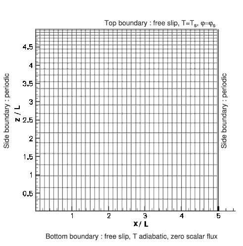
Figure 4: Schematic representation of the computational domain. The scatter shows every $10^{th}$ grid line of the major grid used for the velocity field. The mesh for the scalar was further refined by factors of $R=2,3$ and $5$.

The base grid size was $n_{x}=400$ and $n_{z}=256$ in the $x$- and $z$-directions, respectively. The mesh was stretched in the $z$-direction with $\delta=3$ to obtain a finer resolution near the top where a steep concentration gradient occurs. The general stretching procedure has been given in (28). For all variables, periodic boundary conditions were employed in the horizontal direction. For the velocity field free-slip boundary conditions were used at the top and bottom of the computational domain. At the beginning of each simulation all velocity components were set to zero. The full set of 2D equations for the velocity given in (2) to (6) is solved. It should be noted that to account for the effects of buoyancy in our application case the buoyancy term $\beta(T^{*})$ is included into equation (6) so that $c$ reads

$$c = -\frac{\partial w^{2}}{\partial z}-\frac{\partial uw}{\partial x}+\frac{1}{Re}\left\{\frac{\partial^{2}w}{\partial x^{2}}+\frac{\partial^{2}w}{\partial z^{2}}\right\}+\beta(T^{*}).$$ (34)

The term $\beta(T^{*})$ is modelled using the Boussinesq approximation and is a function of the non-dimensional temperature $T^{*}$ defined as

$$T^{*}=\frac{T-T_{s}}{T_{B,0}-T_{s}}$$ (35)

where the temperature at the top of the domain was set to a fixed value of $T=T_{s}=20$℃ , see (24), while in the rest of the computational domain the initial bulk temperature $T_{B,0}$ was 23℃. The relation between density and temperature within this range can be assumed to be linear. To avoid heat losses, at the bottom of the computational domain an adiabatic boundary condition (25) was employed for $T$. The temperature $T$ is a scalar and hence treated the same as $\varphi$, see (1).

At the top of the computational domain the scalar $\varphi$ was kept at a value of $\varphi=\varphi_{s}$ (24) while at the bottom a zero-flux boundary condition (25) was employed. The scalar was non-dimensionalized using the scalar magnitude at the top boundary $\varphi_{s}$ and the initial magnitude in the bulk $\varphi_{B,0}=0$ so that

$$\varphi^{*}=\frac{\varphi-\varphi_{B,0}}{\varphi_{s}-\varphi_{B,0}}.$$ (36)

The convective instability was triggered by adding random disturbances to the temperature field after letting it evolve for $t=11$ seconds in order to avoid the triggering of the instability to depend on the mesh size or numerical round off error. The same disturbance field was used in all simulations. The random numbers that were added to $T^{*}$ were uniformly distributed between $0$ and $T_{ran}$. To test the influence of the level of the random disturbances on the development of the instability, a test was performed in which a random disturbance field was rescaled so that $T_{ran}=0.010$, $T_{ran}=0.020$ and $T_{ran}=0.040$ before it was added to the non-dimensional temperature. In all three simulations exactly the same buoyant convective disturbance field was found to develop. As can be seen in Table 6,

$T_{ran}$	time at which the falling plume reaches z=4.0 cm
0.010	23.75 s
0.020	22.30 s
0.040	20.85 s

Table 6: The time difference found between the development of disturbances.

the different levels of disturbances were found to affect the time it takes for the plumes to develop. Based on the time difference of 1.45 seconds between subsequent simulations (in which the level of random disturbances is doubled) the exponential growth factor $\lambda$ for the buoyant-convective instability was estimated to be $\lambda=0.478$.

To facilitate the comparison between various simulations involving buoyant convection, in the simulations discussed below (with the exception of Section 5.4) the same random temperature field consisting of uniformly distributed random numbers between $T=0$ and $T_{ran}=0.020$ was added to the non-dimensional temperature field.

5.1 Comparison of scalar convection methods in 2D

As mentioned briefly in Section 3.1 although the fifth-order upstream central method (C5) shows better accuracy on coarse meshes, it is not the method of choice for the current application due to the absence of a mechanism to deal with steep gradients which could result in the appearance of wiggles. To demonstrate this we performed a number of initial 2D simulations on the $400\times 256$ base mesh using the C5 and the WENO5 schemes discussed in Section 3.

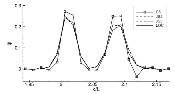
Figure 5: Comparison of WENO5 schemes (JS2, JS3, LOC) and the fifth-order central scheme (C5), showing profiles of the scalar distribution $\varphi$ at $z=4.5$cm and $t=45$ seconds using a Schmidt number of $Sc=500$.

Figure 5 shows the profiles extracted at a cross section at $z=4.5$ cm and $t=45$ seconds obtained for the C5 scheme and different variants of the WENO5 scheme. The cross-section intersects with the falling plumes that develop due to the convective instability which induces sharp gradients in the scalar distribution (see also Figure 7a). The plot reveals that wiggles appear close to steep gradients when using the C5 method. It was found that the wiggles completely disappear when we use the WENO5 schemes JS2 and JS3 of Jiang and Shu [10] with powers $r=2$ and $3$, respectively - see (13,14) - as well as the original implementation of Liu et al. [13] (LOC). It can be seen that the results obtained using the WENO5 schemes are very similar.

In the following sections, the mesh sensitivity for resolving the 2D flow and concentration fields were tested in several subgrid mesh refinement studies.

5.2 Mesh sensitivity test : Flow-field

To verify that the flow-field was fully resolved on the chosen $400\times 256$ base mesh, the grid was refined in all directions by factors of 1.5 and 2, respectively. Fig. 6

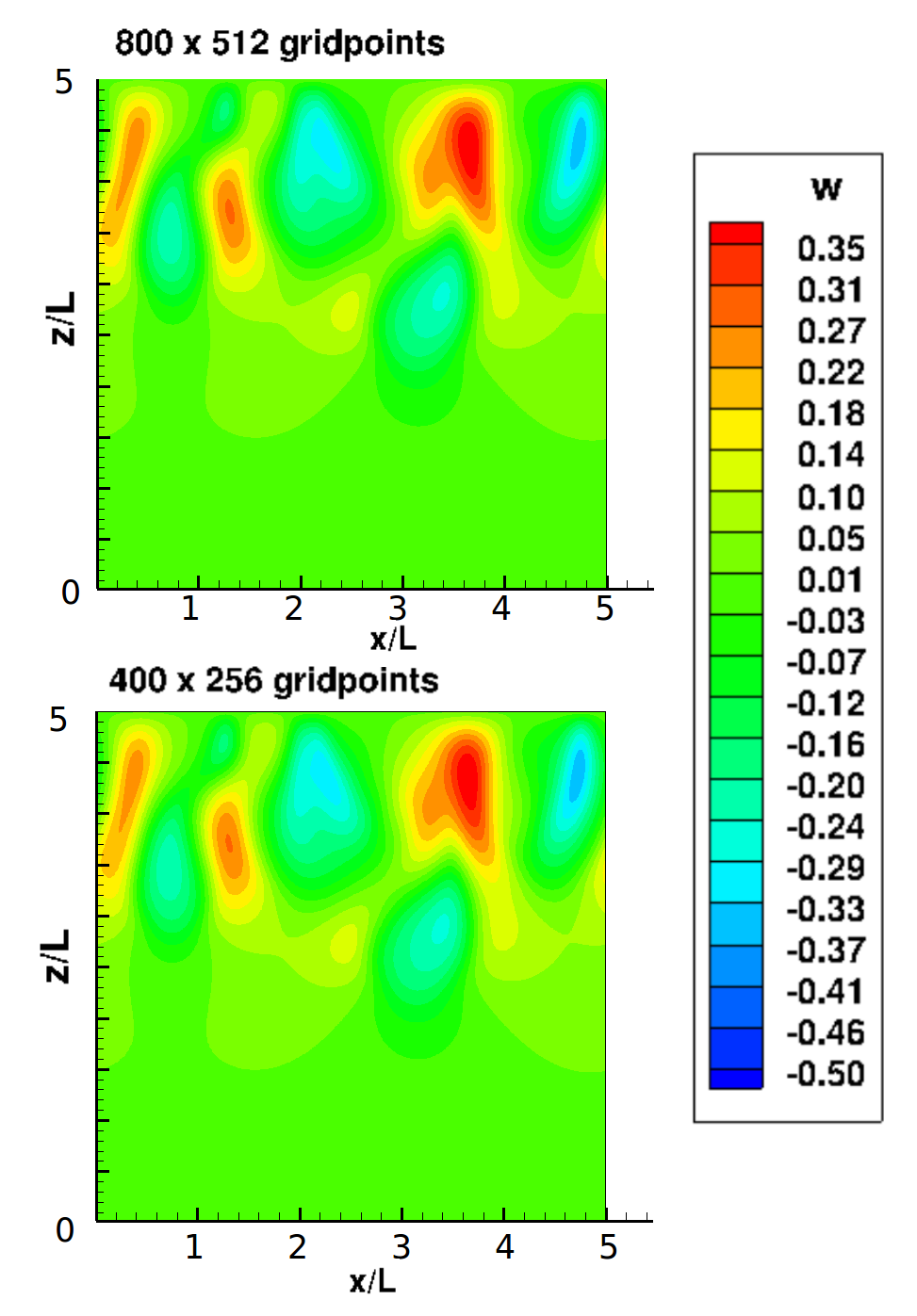
(a) vertical velocity $w$ field on a grid $400\times 256$ and $800\times 512$ after $t=45~{}$seconds

(b) vertical velocity $w$ along a line at $z=4L$ after $t=45~{}$seconds

Figure 6: A grid refinement showed that the velocity field is fully resolved on a $400\times 256$ grid.

shows the contour plots and the velocity profile obtained from the simulations with the base grid and the mesh refined by a factor 2 ($R=2$) (with $800\times 512$ points) after $t=45~{}$seconds. The contour plots of the flow-field using the refined mesh did not show any visible changes in the flow structures (Fig. 6b). This is further confirmed by the vertical velocity profiles along a horizontal line at $z=4L$. The profiles show a nice convergence verifying that the velocity field is fully resolved on the $400\times 256$ grid which was subsequently used in all further cases.

5.3 Mesh sensitivity test : gas concentration field

As described above, we used a dual-mesh approach in which the scalar was resolved on a finer mesh than the one used for the velocity. Various levels of refinement were employed as illustrated in Fig 2. In this section, the mesh sensitivity for the scalar transport using this dual mesh approach is evaluated. Fig. 7

(a) Domain after t = 45 seconds on standard mesh

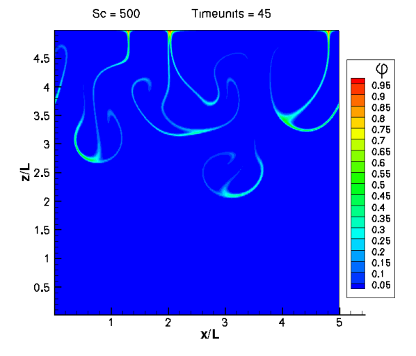
(b) Domain after t = 45 seconds with refined submesh $R=3$

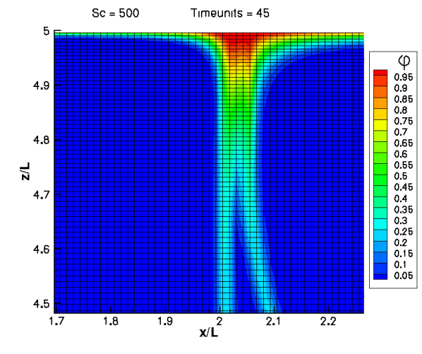
(c) Zoomed view after t = 45 seconds on standard mesh

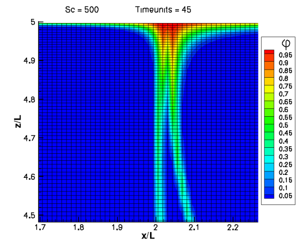
(d) Zoomed view after t = 45 seconds with refined submesh $R=3$

Figure 7: Comparison of the gas concentration field after t = 45 seconds on standard mesh $n_{x}=400$ and $n_{z}=256$ and with a dual subgrid in place three times as fine (see Fig. 2c). The gas concentration field is resolved in sharper detail with less smearing.

shows a comparison of the non-dimensional gas concentration contour plots that visualise the development of the scalar transport at $t=45~{}$seconds using the base mesh ($400\times 256$) for both velocity and scalar and the dual mesh approach with refinement factor 3 applied to the scalar. The Schmidt number is $Sc=500$ which is equivalent to the diffusion of oxygen in water.

In general, both concentration fields in Figs. 7a and 7b reveal the same structures of downwards plumes. However, a zoomed view of the top region near the water surface reveals a more detailed representation of the gas concentration field when the dual mesh approach is used (Fig. 7c and 7d). Please note that the gas concentration in all figures is interpolated to the base grid and not shown on the refined mesh used for the scalar transport.

Figs. 8 and  9

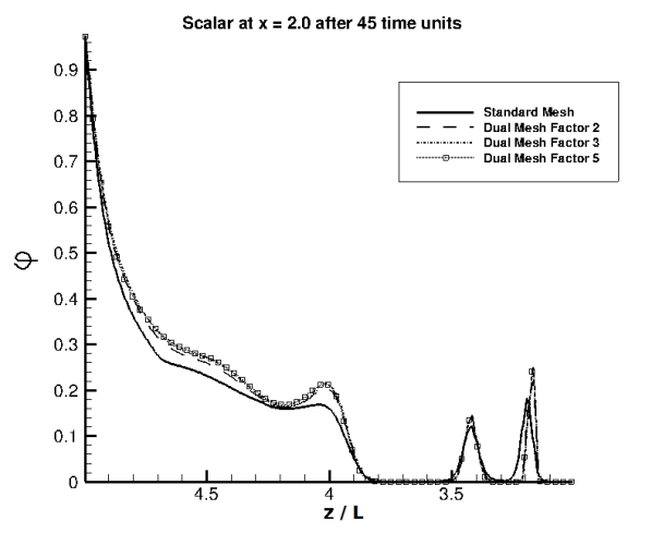
(a) Scalar $\varphi$ for $Sc=500$ at $x=2.0L$

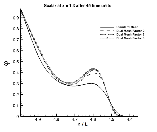
(b) Scalar $\varphi$ for $Sc=500$ at $x=1.3L$

Figure 8: Comparison of scalar field after t = 45 seconds on different levels of subgrid mesh refinement. The two locations are vertical lines at $x=2.0L$ and $x=1.3L$ along the downwards plumes as seen on Fig. 7a.

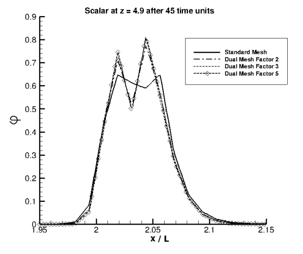
(a) Scalar $\varphi$ for $Sc=500$ at $z=4.9L$

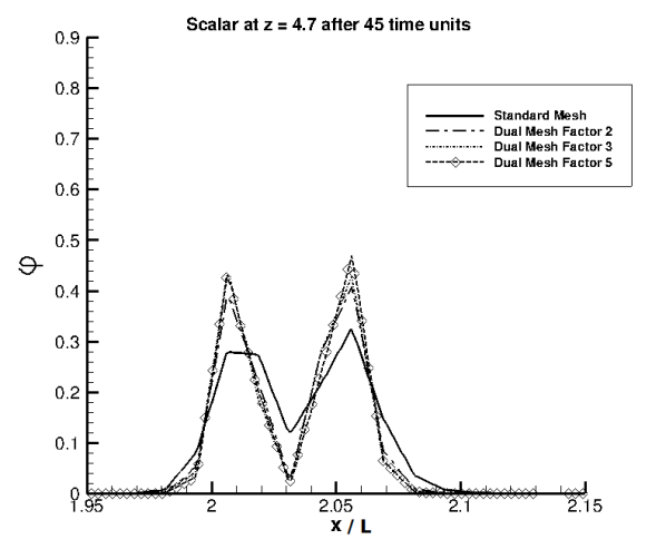
(b) Scalar $\varphi$ for $Sc=500$ at $z=4.7L$

Figure 9: Comparison of scalar field after t = 45 seconds on different levels of subgrid mesh refinement. The location is a horizontal line at various depths $z$ across the downwards plumes as seen on Fig. 7d and 7c.

show line plots of the scalar field at various locations within the domain. The locations are across or along the typical mushroom pattern that develops as a result of the convective instability where sharp gradients in the scalar field are present. Solving the scalar on the finer subgrid shows a significant improvement in resolution. The $R=2$ refinement shows a big improvement in deeper regions where the base mesh is relatively coarse and the scalar distribution is maintained better. In the far field ($z<4$) the scalar concentration profiles for the refined cases $R=2$, $R=3$ and $R=5$ converge to nearly identical values (Fig. 8a).

The improved resolution becomes even more relevant when the spatially integrated total scalar concentration in the domain over time is considered. Fig. 10a

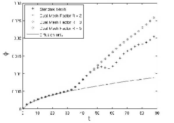
(a) Scalar $\varphi$ for $Sc=500$ over time

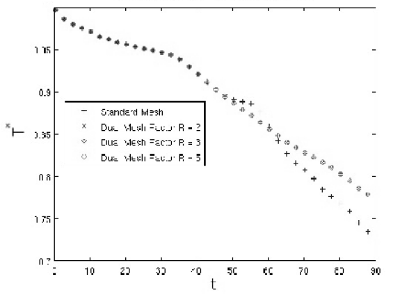
(b) Non-dimensional total temperature $T^{*}$ over time

Figure 10: Comparison of the total non-dimensional scalar concentration and temperature $T^{*}$over time for different levels of subgrid refinement

shows the total concentration over time for $Sc=500$. Up to a time of $t=30~{}$seconds the gas transfer is dominated by diffusion. Subsequently, the instability induces a convective flow that enhances the mass transfer. The typical mushroom patterns start penetrating the deeper regions of the domain. It is here where the refined submesh shows a much improved resolution with a continuous increase in the concentration levels whilst the standard mesh shows a drop in concentration levels. The drop occurs when the scalar reaches the region for $z<2.5L$ (where the mesh becomes significantly coarser) after around $t=55~{}$seconds (Fig. 10a). This points out an insufficient resolution of the scalar transport in this region. This effect was not present in the refined cases (Fig. 10a). The same is found for the transport of the non-dimensionalized temperature $T^{*}$ (Fig. 10b). The grid refinement study for the temperature transport shows a similar trend as seen for the concentration field in Fig. 10b. On the coarse mesh fluctuations become evident after $t=50~{}$seconds whereas the refined cases do not exhibit such temperature fluctuations. Again the results are identical for all refined cases ($R=2$, $R=3$ and $R=5$).

5.4 Comparison to Experiments

In this section we compare the obtained scalar field with the laboratory measurements conducted by Jirka et al. [11] at KIT. In the experiments instantaneous 2D oxygen concentration fields were visualized using a Laser Induced Fluorescence (LIF) technique. The experiments were performed in a $50\times 50\times 65$ cm³ tank and the water depth was about $42$ cm. The surface temperature was 3 ℃  lower than the bulk temperature of the water. The equivalent temperature boundary condition was applied in the numerical simulations.

Fig. 11

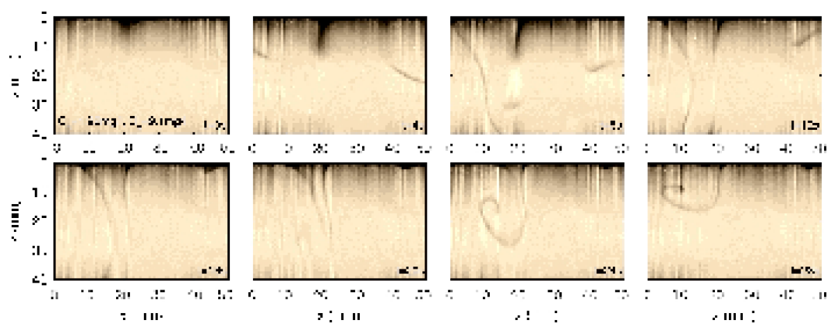
(a) Experimental Results

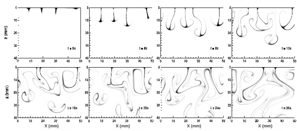
(b) Numerical Results

Figure 11: Comparison of flow structures. High oxygen concentration plumes of LIF measurements conducted by Jirka et al. [11] (Fig. 11a) and DNS results (Fig. 11b). The dark and light colour scaling indicate regions with high and low scalar concentration, respectively. In both cases the surface temperature was 3℃  colder than the bulk temperature.

shows a comparison of 2D-LIF images to 2D DNS results where a refinement factor of $R=2$ has been used. Identical boundary conditions were employed as in the simulations described in the beginning of Section 5.

Note that the DNS results show the top section of the domain that has the same dimension as the LIF-maps. The actual experimental domain was much larger so the sides and bottom in these plots can be considered as open boundaries. For reasons of better comparison the timescale was set to $t=0~{}$seconds from the moment when the flow field started moving which was after a simulation time of 33 seconds. Though the numerical results are only 2D, whereas the real problem is of course 3D, a very good qualitative agreement with the experiment is observed. Both the spatial distance between high concentration plumes and the size of the eddies were found to be similar in the experiment and the simulation. Because of the low diffusivity of oxygen in water and the rather low turbulent flow the plumes of high oxygen concentration retain their fine structures. This means that the steep concentration gradients do not smear out because of excessive numerical diffusion. As a result good qualitative agreement between the numerical simulations and the experimental data is obtained.

6 Conclusion

To accurately resolve the mass transport for a scalar with low diffusivity on a stretched and staggered mesh, the fifth-order accurate WENO5 schemes of Liu et al. [13] and Jiang and Shu [10] was implemented to discretize the convective terms, while a fourth order accurate central discretization was used for the diffusion. The flow field was approximated by fourth-order accurate central discretizations for both convection and diffusion. Because the diffusivity of the scalars of interest is up to almost three orders of magnitude smaller than the molecular diffusivity of the ambient fluid, the resolution requirements for the transported scalar are much higher. Hence, to save computing time, a dual meshing approach was employed in which the scalar transport equations were discretized on a finer mesh than the flow field. The discretization of scalar convection and diffusion were tested in both 1D and 2D cases. The 1D tests showed that the spatial discretization of the scalar convection achieved a second-order accuracy on non-uniform meshes and a fifth-order accuracy on uniform meshes, while the discretization of the diffusive term was shown to achieve a fourth-order accuracy on stretched meshes. Though the WENO5 implementation of Jiang & Shu [10] shows superior results in the grid refinement tests, the original scheme of Liu at al. [13] was found to be more accurate on coarse meshes. Hence, to obtain a satisfactory resolution of the steep concentration gradients - that will occur in scalar transport problems with high Schmidt numbers - using as few grid points as possible, the Liu et al. implementation was found to be a good choice.

For the 2D case a combined active and passive scalar transport problem was simulated. It was shown that the fifth-order central upwind method generated wiggles near steep gradients which completely disappeared when using the WENO5 schemes. The dual meshing approach showed a significant improvement in accuracy of the scalar field resolution even for a moderate refinement by a factor of two. Subsequent refinements that were carried out using factors of up to five times only showed marginal further improvements in accuracy. Additionally, a qualitative comparison of the numerical results to experimentally visualized oxygen concentration fields in water showed similar structures below the air-water interface even though the numerical simulations were 2-dimensional.

References

- Balsara and Shu [2000] D.S. Balsara and C-W. Shu. Monotonicity preserving WENO schemes with increasingly high-order of accuracy. J. Comput. Phys., 160(2):405–452, 2000.
- Banerjee [2007] S. Banerjee. Modeling of interphase turbulent transport processes. Ind. Eng. Chem. Res., 46(10):3063–3068, 2007.
- Banerjee et al. [2004] S. Banerjee, D. Lakehal, and M. Fulgosi. Surface divergence models for scalar exchange between turbulent streams. Int.J.Multiphas. Flow, 30(7-8):963–977, 2004.
- Borges et al. [2008] R. Borges, M. Carmona, B. Costa, and W.S. Don. An improved WENO scheme for hyperbolic conservation laws. J. Comput. Phys., 227(6):3191–3211, 2008.
- Collatz [1960] L. Collatz. The Numerical Treatment of Differential Equations. Springer, Berlin, 3rd edition, 1960.
- Handler et al. [1999] R.A. Handler, J.R. Saylor, R.I. Leighton, and A.L. Rovelstad. Transport of a passive scalar at a shear-free boundary in fully developed turbulent open channel flow. Phys. Fluids, 11(9), 1999.
- Harten et al. [1987] A. Harten, B. Engquist, S. Osher, and S.R. Chakravarthy. Uniformly high-order accurate essentially non-oscillatory schemes, III. J. Comput. Phys., 71(2):231–303, 1987.
- Hasegawa and Kasagi [2009] Y. Hasegawa and N. Kasagi. Hybrid DNS/LES of high Schmidt number mass transfer across turbulent air-water interface. Int. J. Heat Fluid Fl., 52(3-4):1012–1022, 2009.
- Henrick et al. [2005] A.K. Henrick, T.D. Aslam, and J.M. Powers. Mapped weighted essentially non-oscillatory schemes: Achieving optimal order near critical points. J. Comput. Phys., 207(1):542–567, 2005.
- Jiang and Shu [1996] G.S. Jiang and C-W. Shu. Efficient implementation of weighted ENO schemes. J. Comput. Phys., 126(1):202–228, 1996.
- Jirka et al. [2010] G.H. Jirka, H. Herlina, and A. Niepelt. Gas transfer at the air-water interface: experiments with different turbulence forcing mechanisms. Exp. Fluids, 49(1):319–327, 2010.
- Johnsen and Colonius [2006] E. Johnsen and T. Colonius. Implementation of WENO schemes in compressible multicomponent flow problems. J. Comput. Phys., 219(2):715–732, 2006.
- Liu et al. [1994] X.D. Liu, S. Osher, and T. Chan. Weighted essentially non-oscillatory schemes. J. Comput. Phys., 115(1):200–212, 1994.
- Martin et al. [2006] M.P. Martin, E.M. Taylor, M. Wu, and V.G. Weirs. A bandwidth-optimized WENO scheme for effective direct numerical simulation of compressible turbulence. J. Comput. Phys., 220(1):270–289, 2006.
- Schwertfirm and Manhart [2007] F. Schwertfirm and M. Manhart. DNS of passive scalar transport in turbulent channel flow at high Schmidt numbers. Int. J. Heat Fluid Fl., 28(6):1204–1214, 2007.
- Schwertfirm et al. [2008] F. Schwertfirm, J. Mathew, and M. Manhart. Improving spatial resolution characteristics of finite difference and finite volume schemes by approximate deconvolution pre-processing. Comput. Fluids, 37(9):1092–1102, 2008.
- Sharif and Busnaina [1988] M.A.R. Sharif and A.A. Busnaina. An investigation into the numerical dispersion problem of the skew upwind finite difference scheme. Appl. Math.Model., 12(2):98–108, 1988.
- Shu and Osher [1988] C-W. Shu and S. Osher. Efficient implementation of essentially non-oscillatory shock-capturing schemes. J. Comput. Phys., 77(1):439–471, 1988.
- Tadmor [1990] E. Tadmor. Shock capturing by the spectral viscosity method. Comput. Meth. Appl. Mech. Eng., 80(1-3):197–208, 1990.
- Wissink [2004] J.G. Wissink. On unconditional conservation of kinetic energy by finite-difference discretizations of the linear and non-linear convection equation. Comput.Fluids, 33(2):315–343, 2004.