Linear magnetoresistance on the topological surface

Abstract

A positive, non-saturating and dominantly linear magnetoresistance is demonstrated to occur in the surface state of a topological insulator having a wavevector-linear energy dispersion together with a finite positive Zeeman energy splitting. This linear magnetoresistance shows up within quite wide magnetic-field range in a spatially homogenous system of high carrier density and low mobility in which the conduction electrons are in extended states and spread over many smeared Landau levels, and is robust against increasing temperature, in agreement with recent experimental findings in Bi₂Se₃ nanoribbons.

I introduction

It is well known that the classical magnetoresistance (MR) in metals or semiconductors with a closed free electron Fermi surface increases quadratically with increasing magnetic field $B$ for $\mu B\ll 1$ and saturates when $\mu B>1$. Here $\mu$ is the zero-magnetic-field mobility. Hence, the extraordinarily high and linear MR (LMR), which breaks this familiar rule, has been gaining much attention as soon as its discovery. In the past decade, this unexpected LMR has been reported in silver chalcogenide,xu1997large indium antimonide,hu2008classical silicon,delmo2009large MnAs-GaAs composite material,Johnson2010 and graphene.friedman2010quantum

Kapitza’s linear lawKapitza1929 indicates that the metal shows a magnetoresistance linear in perpendicular magnetic field when it has an open Fermi surface and a mean free path longer than the electronic Larmor radius. Recently, another two models, irrespective of the open Fermi surface, have been constructed to provide possible mechanisms for the LMR phenomenon. Abrikosov suggested a quantum-limit origin of LMR for the homogenous system with a gapless linear energy spectrum.Abrikosov1998 ; abrikosov2000quantum His model requires that Landau levels are well formed and the carrier concentration is small that all electrons occupy only the lowest Landau band. Alternatively, Parish and Littlewood developed a classical model without involving linear spectrum.Parish2003 Ignoring the concrete microscopic mechanism, they attributed this unusual MR to the mobility fluctuations in a strongly inhomogenous system.

Topological insulatorsKane2005 ; hasan2010colloquium ; qi2010topological (TIs) are novel materials with a full energy gap in bulk, while there are gapless surface states. Due to its unique band structure with only one helical Dirac cone and linear energy dispersion,xia2009observation ; zhang2009natphys ; CXLiu2010 the surface states of the TI Bi₂Se₃ become an excellent platform for the study of quantum-limit LMR. The recent experiment in this flat surface system, however, reported that a large positive MR, which becomes very linear above a characteristic field of $1$$\sim$$2$ T, was observed even in an opposite situation where the carrier sheet density is high that electrons occupy more than one Landau levels.Tang2011 Moreover, they found that raising temperature to room temperature almost has no influence on the observed LMR. It is striking that this observation is in conflict with Abrikosov’s model and also with the classical Parish-Littlewood model. So far a reliable theoretical scheme capable of explaining this novel experiment has still been lacking.

In this paper, we generalize the balance-equation approachlei1985gsf to a system modeling the surface states of a three-dimensional TI to investigate the two-dimensional magnetotransport in it. We find that a positive, nonsaturating and dominantly linear magnetoresistance can appear within quite wide magnetic-field range in the TI surface state having a positive and finite effective g-factor. This linear magnetoresistance shows up in the system of high carrier concentration and low mobility when electrons are in extended states and spread over many smeared Landau levels, and persists up to room temperature, providing a possible mechanism for the recently observed linear magnetoresistance in topological insulator Bi₂Se₃ nanoribbons.Tang2011

II Balance-Equation Formulation for magnetoresistivity

We consider the surface state of a Bi₂Se₃-type large bulk gap TI in the $x$-$y$ plane under the influence of a uniform magnetic field $\bm{B}$ applied along the $z$ direction.CXLiu2010 Following the experimental observation,Tang2011 we assume that the Fermi energy locates in the gap of the bulk band and above the Dirac point, i.e. the surface carriers are electrons. Further, the separations of the Fermi energy from the bottom of bulk band and Dirac point are much larger than the highest temperature ($300\,{\rm K}$) considered in this work. Hence, the contribution from the bulk band to the magnetotransport is negligible. These electrons, scattered by randomly distributed impurities and by phonons, are driven by a uniform in-plane electric field $\bm{E}=(E_{x},E_{y})$ in the topological surface. The Hamiltonian of this many-electron and phonon system consists of an electron part $\mathcal{H}_{\rm e}$, a phonon part $\mathcal{H}_{\rm ph}$, and electron-impurity and electron-phonon interactions $\mathcal{H}_{\rm ei}$ and $\mathcal{H}_{\rm ep}$:

$$\mathcal{H}=\mathcal{H}_{\rm e}+\mathcal{H}_{\rm ei}+\mathcal{H}_{\rm ep}+\mathcal{H}_{\rm ph}.$$ (1)

Here, the electron Hamiltonian is taken in the form

$$\mathcal{H}_{\rm e}=\sum_{j}\left[v_{\rm F}(\pi_{j}^{x}\sigma_{j}^{y}-\pi_{j}^{y}\sigma_{j}^{x})+\frac{1}{2}g_{z}\mu_{\rm B}B\sigma_{j}^{z}+e\bm{r}_{j}\cdot\bm{E}\right],$$ (2)

in which ${\bm{\pi}}_{j}\equiv\bm{p}_{j}+e\bm{A}(\bm{r}_{j})=(\pi_{j}^{x},\pi_{j}^{y})$, ${\bm{r}}_{j}=(x_{j},y_{j})$, ${\bm{p}}_{j}=(p_{jx},p_{jy})$ and ${\bm{\sigma}}_{j}=(\sigma_{j}^{x},\sigma_{j}^{y},\sigma_{j}^{z})$, stand, respectively, for the canonical momentum, coordinate, momentum and spin operators of the $j$th electron having charge $-e$, $\bm{A}(\bm{r})=(-By,0)$ is the vector potential of the perpendicular magnetic field $\bm{B}=B\hat{z}$ in the Landau gauge, $v_{\rm F}$ is the Fermi velocity, $g_{z}$ is the effective g-factor of the surface electron, and $\mu_{\rm B}=e/2m_{0}$ is the Bohr magneton with $m_{0}$ the free electron mass. The sum index $j$ in Eq. (2) goes over all electrons of total number $N$ in the surface state of unit area.

In the frame work of balance equation approach,lei1985tdb ; lei1985gsf ; cai1985 the two-dimensional center-of-mass (c.m.) momentum and coordinate $\bm{P}=\sum_{j}\bm{p}_{j}$ and $\bm{R}=N^{-1}\sum_{j}\bm{r}_{j}$, and the relative-electron momenta and coordinates $\bm{p}^{\prime}_{j}=\bm{p}_{j}-\bm{P}/N$ and $\bm{r}_{j}^{\prime}=\bm{r}_{j}-\bm{R}$ are introduced to write the Hamiltonian $\mathcal{H}_{\rm e}$ into the sum of a single-particle c.m. part $\mathcal{H}_{\rm cm}$ and a many-particle relative-electron part $\mathcal{H}_{\rm er}$: $\mathcal{H}_{\rm e}=\mathcal{H}_{\rm cm}+\mathcal{H}_{\rm er}$, with

$$\mathcal{H}_{\rm cm} =v_{\rm F}(\varPi_{x}\sigma_{\rm c}^{y}-\varPi_{y}\sigma_{\rm c}^{x})+Ne{\bm{E}}\cdot\bm{R},$$ (3)

$$\mathcal{H}_{\rm er} =\sum_{j}\left[v_{\rm F}(\pi_{j}^{\prime x}\sigma_{j}^{y}-\pi_{j}^{\prime y}\sigma_{j}^{x})+\frac{1}{2}g_{z}\mu_{\rm B}B\sigma_{j}^{z}\right].$$ (4)

In this, ${\bm{\varPi}}\equiv\bm{P}+Ne\bm{A}(\bm{R})=(\varPi_{x},\varPi_{y})$ is the canonical momentum of the center-of-mass and ${\bm{\pi}}_{j}^{\prime}\equiv\bm{p}_{j}^{\prime}+e\bm{A}(\bm{r}_{j}^{\prime})=(\pi_{j}^{\prime x},\pi_{j}^{\prime y})$ is the canonical momentum for the $j$th relative electron. Here we have also introduced c.m. spin operators ${\sigma}_{\rm c}^{x}\equiv N^{-1}\sum_{j}\sigma_{j}^{x}$ and ${\sigma}_{\rm c}^{y}\equiv N^{-1}\sum_{j}\sigma_{j}^{y}$. The commutation relations between the c.m. spin operators $\sigma_{\rm c}^{x}$ and $\sigma_{\rm c}^{y}$ and the spin operators $\sigma_{j}^{x}$, $\sigma_{j}^{y}$ and $\sigma_{j}^{z}$ of the $j$th electron are of order of $1/N$: $[\sigma_{j}^{\beta_{1}},\sigma_{\rm c}^{\beta_{2}}]=N^{-1}2\,{\rm i}\,\varepsilon_{\beta_{1}\beta_{2}\beta_{3}}\sigma_{j}^{\beta_{3}}$ with $\beta_{1},\beta_{2},\beta_{3}=(x,y,z)$. Therefore, for a macroscopic large $N$ system, the c.m. part $\mathcal{H}_{\rm cm}$ actually commutes with the relative-electron part $\mathcal{H}_{\rm er}$ in the Hamiltonian, i.e. the c.m. motion and the relative motion of electrons are truly separated from each other. The couplings between the two emerge only through the electron–impurity and electron–phonon interactions. Furthermore, the electric field ${\bm{E}}$ shows up only in $\mathcal{H}_{\rm cm}$. And, in view of $[r^{\prime}_{i\alpha},p^{\prime}_{j\beta}]={\rm i}\delta_{\alpha\beta}(\delta_{ij}-1/N)\simeq{\rm i}\delta_{\alpha\beta}\delta_{ij}$, i.e. the relative-electron momenta and coordinates can be treated as canonical conjugate variables, the relative-motion part $\mathcal{H}_{\rm er}$ is just the Hamiltonian of $N$ electrons in the surface state of TI in the magnetic field without the presence of the electric field.

In terms of the c.m. coordinate ${\bm{R}}$ and the relative electron density operator $\rho_{\bm{q}}=\sum_{j}{\rm e}^{{\rm i}\,{\bm{q}}\cdot{\bm{r}}^{\prime}_{j}}$, the electron–impurity and electron–phonon interactions can be written aslei1985tdb ; cai1985

$$\mathcal{H}_{\rm ei}= \sum_{{\bm{q}},a}U({\bm{q}})\,{\rm e}^{{\rm i}\,{\bm{q}}\cdot\left({\bm{R}}-{\bm{r}}_{a}\right)}\rho_{{\bm{q}}},$$ (5)

$$\mathcal{H}_{\rm ep}= \sum_{{\bm{Q}},\lambda}M({\bm{Q}},\lambda)\,\phi_{{\bm{Q}}\lambda}{\rm e}^{{\rm i}\,{\bm{q}}\cdot{\bm{R}}}\rho_{{\bm{q}}}.$$ (6)

Here $U({\boldsymbol{q}})$ and $M({\boldsymbol{Q}},\lambda)$ are respectively the impurity potential (an impurity at randomly distributed position ${\bm{r}}_{a}$) and electron–phonon coupling matrix element in the plane-wave representation, and $\phi_{{\bm{Q}}\lambda}\equiv b_{{\bm{Q}}\lambda}+b_{-{\bm{Q}}\lambda}^{\dagger}$ with $b_{{\boldsymbol{Q}}\lambda}^{\dagger}$ and $b_{{\bm{Q}}\lambda}$ being the creation and annihilation operators for a phonon of wavevector ${\bm{Q}}=({\bm{q}},q_{z})$ in branch $\lambda$ having frequency ${\it\Omega}_{{\bm{Q}}\lambda}$.

The c.m. velocity (operator) ${\bm{V}}$ is the time variation of its coordinate: ${\bm{V}}=\dot{\bm{R}}=-{\rm i}[{\bm{R}},\mathcal{H}]=v_{\rm F}(\sigma_{\rm c}^{y}\,\hat{i}-\sigma_{\rm c}^{x}\,\hat{j})$. To derive a force-balance equation for steady state transport we consider the Heisenberg equation for the rate of change of the c.m. canonical momentum $\bm{\varPi}$:

$$\dot{\bm{\varPi}}=-{\rm i}\,[{\bm{\varPi}},\mathcal{H}]=-Ne({\bm{V}}\times{\bm{B}})-Ne{\bm{E}}+{\bm{F}}_{\rm i}+{\bm{F}}_{\rm p},$$ (7)

in which the frictional forces ${\bm{F}}_{\rm i}$ and ${\bm{F}}_{\rm p}$ share the same expressions as given in Ref. cai1985, .

The statistical average of the operator equation (7) can be determined to linear order in the electron–impurity and electron–phonon interactions $\mathcal{H}_{\rm ei}$ and $\mathcal{H}_{\rm ep}$ with the initial density matrix $\hat{\rho}_{0}=Z^{-1}e^{-(\mathcal{H}_{\rm ph}+\mathcal{H}_{\rm er})/T}$ at temperature $T$ when the in-plane electric field ${\bm{E}}$ is not strong. For steady-transport states we have $\langle\dot{\bm{\varPi}}\rangle=0$, leading to a force-balance equation of the form

$$0=-Ne\bm{v}\times\bm{B}-Ne\bm{E}+\bm{f}_{\rm i}+\bm{f}_{\rm p}.\\$$ (8)

Here ${\bm{v}}=\langle{\bm{V}}\rangle$, the statistically averaged velocity of the moving center-of-mass, is identified as the average rate of change of its position, i.e. the drift velocity of the electron system driven by the electric field ${\bm{E}}$, and $\bm{f}_{\rm i}$ and $\bm{f}_{\rm p}$ are frictional forces experienced by the center-of-mass due to impurity and phonon scatterings:

$$\bm{f}_{\rm i}= \sum_{\bm{q}}\left|U(\bm{q})\right|^{2}\bm{q}\varPi_{2}(\bm{q},\omega_{0}),$$ (9)

$$\bm{f}_{\rm p}= \sum_{\bm{Q},\lambda}\left|M(\bm{Q},\lambda)\right|^{2}\bm{q}\varPi_{2}(\bm{q},{\it\Omega}_{\bm{Q}\lambda}+\omega_{0})$$

$$\hskip 11.38092pt\times\left[n\Big{(}\frac{{\it\Omega}_{\bm{Q}\lambda}}{T}\Big{)}-n\Big{(}\frac{{\it\Omega}_{\bm{Q}\lambda}+\omega_{0}}{T}\Big{)}\right],$$ (10)

in which $n(x)=(e^{x}-1)^{-1}$ is the Bose distribution function, $\omega_{0}\equiv{\bm{q}}\cdot{\bm{v}}$, and $\varPi_{2}(\bm{q},\omega)$ stands for the imaginary part of the Fourier spectrum of the relative-electron density correlation function defined by

$$\varPi({\bm{q}},t-t^{\prime})=-{\rm i\,}\theta(t-t^{\prime})\big{\langle}\big{[}\rho_{{\bm{q}}}(t),\,\rho_{-{\bm{q}}}(t^{\prime})\big{]}\big{\rangle}_{0},$$ (11)

where $\rho_{{\bm{q}}}(t)={\rm e}^{{\rm i\,}\mathcal{H}_{\rm er}t}\rho_{{\bm{q}}}\,{\rm e}^{-{\rm i\,}\mathcal{H}_{\rm er}t}$ and $\langle...\rangle_{0}$ denotes the statistical averaging over the initial density matrix $\hat{\rho}_{0}$.lei1985gsf

The force-balance equation (8) describes the steady-state two-dimensional magnetotransport in the surface state of a TI. Note that the frictional forces $\bm{f}_{\rm i}$ and $\bm{f}_{\rm p}$ are in the opposite direction of the drift velocity $\bm{v}$ and their magnitudes are functions of $v=|{\bm{v}}|$ only. With the drift velocity $\bm{v}=(v,0)$ in the $x$ direction, the force-balance equation Eq. (8) yields a transverse resistivity $R_{xy}=-E_{y}/(Nev)=-B/(Ne)$, and a longitudinal resistivity $R_{xx}=-E_{x}/(Nev)=-(f_{\rm i}+f_{\rm p})/(N^{2}e^{2}v)$. The linear one is in the form

$$R_{xx}= -\frac{1}{N^{2}e^{2}}\sum_{\bm{q}}|U(\bm{q})|^{2}q_{x}^{2}\frac{\partial}{\partial\omega}\varPi_{2}(\bm{q},\omega)\big{|}_{\omega=0}$$

$$-\frac{1}{2TN^{2}e^{2}}\sum_{\bm{Q},\lambda}|M(\bm{Q},\lambda)|^{2}q_{x}^{2}\varPi_{2}(\bm{q},{\it\Omega}_{\bm{Q}\lambda})$$

$$\hskip 85.35826pt\times{\rm csch}^{2}\Big{(}\frac{{\it\Omega}_{\bm{Q}\lambda}}{2T}\Big{)}.$$ (12)

III Density correlation function in the Landau representation

For calculating the electron density correlation function $\varPi_{2}(\bm{q},\omega)$ we proceed in the Landau representation.cai1985 ; Ting1977 The Landau levels of the single-particle Hamiltonian $h=v_{\rm F}(\pi^{x}\sigma^{y}-\pi^{y}\sigma^{x})+\frac{1}{2}g_{z}\mu_{\rm B}B\sigma^{z}$ of the relative-electron system in the absence of electric field are composed of a positive “$+$” and a negative “$-$” branchMcClure1956 ; Zheng2002 ; ZGWang2010 ; Zarea2005 ; Taskin2011

$$\varepsilon_{n}^{\pm}=\pm\sqrt{2n\varepsilon_{s}^{2}+\delta_{z}^{2}}=\pm\varepsilon_{n}\,\,\,(n=1,2,....)$$ (13)

with $\varepsilon_{s}=v_{F}\sqrt{eB}$ and $\delta_{z}=-\frac{1}{2}g_{z}\mu_{\rm B}B$, and a zero ($n=0$) level

$$\varepsilon_{0}=\delta_{z}=-\frac{1}{2}g_{z}\mu_{\rm B}B.$$ (14)

The corresponding Landau wave functions are

$$\Psi_{n,k_{x}}^{+}(\bm{r})=\frac{1}{\sqrt{\mathcal{R}_{n}}}e^{ik_{x}x}\left(\begin{array}[]{c}{\rm i}\mathcal{P}_{n}\phi_{{n-1},k_{x}}(y)\\ \phi_{n,k_{x}}(y)\\ \end{array}\right)$$ (15)

and

$$\Psi_{n,k_{x}}^{-}(\bm{r})=\frac{1}{\sqrt{\mathcal{R}_{n}}}e^{ik_{x}x}\left(\begin{array}[]{c}\phi_{{n-1},k_{x}}(y)\\ {\rm i}\mathcal{P}_{n}\phi_{n,k_{x}}(y)\\ \end{array}\right)$$ (16)

for $n=1,2,...$; and

$$\Psi_{0,k_{x}}(\bm{r})=e^{{\rm i}k_{x}x}\left(\begin{array}[]{c}0\\ \phi_{0,k_{x}}(y)\\ \end{array}\right)$$ (17)

for $n=0$. Here $k_{x}$ is the wavevector of the system along $x$ direction; $\mathcal{R}_{n}=1+\mathcal{P}_{n}^{2}$ with $\mathcal{P}_{n}=\sqrt{2n}\varepsilon_{s}/(\delta_{z}+\sqrt{2n\varepsilon_{s}^{2}+\delta_{z}^{2}})$; and $\phi_{n,k_{x}}(y)=D_{n}\exp(-\gamma^{2}/2)H_{n}(\gamma)$ is the harmonic oscillator eigenfunction with $H_{n}(x)$ being the Hermite polynomial, $\gamma\equiv(y-y_{c})/l_{\rm B}=\sqrt{eB}(y-k_{x}l_{\rm B}^{2})$, and $D_{n}=1/(2^{n}n!)^{1/2}(eB/\pi)^{1/4}$.

Each Landau level contains $n_{\rm B}=eB/2\pi=1/(2\pi l_{\rm B}^{2})$ electron states for system of unit surface area. The positive branch $\varepsilon_{n}^{+}=\varepsilon_{n}$ and the $n=0$ level $\varepsilon_{0}$ of the above energy spectra are indeed quite close to those of the surface states in the bulk gap of Bi₂Se₃-family materials derived from microscopic band calculation.CXLiu2010

The Landau levels are broadened due to impurity, phonon and electron-electron scatterings. We model the imaginary part of the retarded Green’s function, or the density-of-states, of the broadened Landau level $n$ (written for “+”-branch and $n=0$ levels), using a Gaussian-type form:Ando1982

$${\rm Im}G_{n}(\epsilon)=-\frac{\sqrt{2\pi}}{\varGamma}\exp\left[-\frac{2(\epsilon-\varepsilon_{n})^{2}}{\varGamma^{2}}\right],$$ (18)

with a half-width ${\it\Gamma}$ of the form:Zheng2002 $\varGamma=\left[{2\omega_{c}}/({\pi\tau_{s}})\right]^{1/2}$. Here $\tau_{s}$ is the single-particle lifetime and $\omega_{c}=eBv_{\rm F}^{2}/\varepsilon_{\rm F}^{0}$ is the cyclotron frequency of linear-energy-dispersion system with $\varepsilon_{\rm F}^{0}=2v_{\rm F}\sqrt{\pi N}$ being the zero-temperature Fermi level. Using a semi-empirical parameter $\alpha$ to relate $\tau_{s}$ with the transport scattering time $\tau_{\rm tr}=4\alpha\tau_{s}$, and expressing $\tau_{\rm tr}$ with the zero-field mobility $\mu$ at finite temperature,Dimitrie we can write the Landau-level broadening as

$$\varGamma=(ev_{\rm F}/\pi)[2B\alpha/(N\mu)]^{1/2}.$$ (19)

In the present study we consider the case of $n$-doping, i.e. the Fermi level is high enough above the energy zero of the Dirac cone in the range of “+”-branch levels and the states of “$-$”-branch levels are completely filled, that they are irrelevant to electron transport.

Special attention has to be paid to the $n=0$ level, since, depending on the direction of exchange potential the effective g-factor of a TI surface state, $g_{z}$, can be positive, zero or negative.ZGWang2010 ; Taskin2011 The sign and magnitude of the effective g-factor determines how many states of the zero level should be included in or excluded from the available states for electron occupation in the case of $n$-doping at a magnetic field. (i) If $g_{z}=0$, the $n=0$ level center is exactly at $\varepsilon_{0}=0$ and the system is electron-hole symmetric. The total number of negative energy states (including the states of the lower half of the $n=0$ level and states of the “$-$”-branch levels) and that of positive energy states (including the states of the upper half of the $n=0$ level and states of the “$+$”-branch levels) do not change when changing magnetic field. Therefore, the lower-half negative energy states of this level are always filled and the upper-half positive-energy states of it are available for the occupation of particles which are counted as electrons participating in transport in the case of $n$-doping. (ii) For a finite positive $g_{z}>0$, the $n=0$ level $\varepsilon_{0}$ moves downward to negative energy and its distance to the nearest “$-$”-branch level is $2|\delta_{z}|=g_{z}\mu_{\rm B}B$ closer than to the nearest “+”-branch level at finite magnetic field strength $B$. This is equivalent to the opening of an increasingly enlarged (with increasing $B$) energy gap between the “+”-branch states and the states of the zero-level and the “$-$”-branch levels. The opening of a sufficient energy gap implies that with increasing magnetic field the states in the “+”-branch levels would no longer shrink into the zero-level, and thus the $n=0$ level should be completely excluded from the conduction band, i.e. only particles occupying the “+”-branch states are counted as electrons participating in transport in the case of $n$-doping, when the magnetic field $B$ gets larger than a certain value (depending on the magnitude of $g_{z}$). (iii) For a finite negative $g_{z}<0$, the $n=0$ level $\varepsilon_{0}$ moves upward to positive energy and an increasingly enlarged energy gap will be opened between the states of the zero-level and the “+”-branch and the states of “$-$”-branch levels, and particles occupying the $n=0$ level and “+”-branch states are electrons participating in transport when the magnetic field $B$ gets larger than a certain value.

As a result, the experimentally accessible sheet density $N$ of electrons participating in transport is related to the Fermi energy $\varepsilon_{\rm F}$ by the following equation valid at finite $g_{z}$ for the magnetic field $B$ larger than a certain value:

$$N=-\frac{1}{2(\pi l_{\rm B})^{2}}\int d\epsilon f(\epsilon)\sum_{n}^{\infty}{\rm Im}G_{n}(\epsilon),$$ (20)

in which $f(\epsilon)=\{\exp[(\epsilon-\varepsilon_{\rm F})/T]+1\}^{-1}$ is the Fermi distribution function at temperature $T$ and the summation index $n$ goes over $(1,2,....)$ for $g_{z}>0$, or $(0,1,2,....)$ for $g_{z}<0$. In the case of $g_{z}=0$,

$$N=-\frac{1}{2(\pi l_{\rm B})^{2}}\int d\epsilon f(\epsilon)\bigg{[}\sum_{n=1}^{\infty}{\rm Im}G_{n}(\epsilon)+{\rm Im}G_{0}^{p}(\epsilon)\bigg{]}$$ (21)

valid for arbitrary magnetic field, in which ${\rm Im}G_{0}^{p}(\epsilon)={\rm Im}G_{0}(\epsilon)\theta(\epsilon)$.

The imaginary part of relative-electron density correlation function in the presence of a magnetic field, $\varPi_{2}(\bm{q},\omega)$, can be expressed in the Landau representation asTing1977 ; cai1985

$$\varPi_{2}(\bm{q},\omega)=\frac{1}{2\pi l_{\rm B}^{2}}\sum_{n,n^{\prime}}C_{n,n^{\prime}}(l_{\rm B}^{2}q^{2}/2)\varPi_{2}(n,n^{\prime},\omega),$$ (22)

in which the transform factor

$$C_{n,n^{\prime}}(\xi)\equiv \frac{e^{-\xi}\xi^{n_{2}-n_{1}}}{\mathcal{R}_{n}\mathcal{R}_{n^{\prime}}}\frac{n_{1}!}{n_{2}!}\bigg{[}L_{n_{1}}^{n_{2}-n_{1}}(\xi)$$

$$\hskip 28.45274pt+s_{n}s_{n^{\prime}}\mathcal{P}_{n}\mathcal{P}_{n^{\prime}}\sqrt{\frac{n_{2}}{n_{1}}}L_{n_{1}-1}^{n_{2}-n_{1}}(\xi)\bigg{]}^{2},$$ (23)

with $n_{1}={\rm min}(n,n^{\prime})$, $n_{2}={\rm max}(n,n^{\prime})$, $s_{n}=1-\delta_{n,0}$, and $L_{n}^{m}(x)$ being associated Laguerre polynomials. The Landau-representation correlation function $\varPi_{2}(n,n^{\prime},\omega)$ in Eq. (22) can be constructed with the imaginary part of the retarded Green’s function ${\rm Im}G_{n}(\epsilon)$, or the density-of-states, of the $n$th Landau level asTing1977 ; cai1985

$$\varPi_{2}(n,n^{\prime},\omega)= -\frac{1}{\pi}\int d\epsilon[f(\epsilon)-f(\epsilon+\omega)]$$

$$\hskip 34.14322pt\times{\rm Im}G_{n}(\epsilon+\omega){\rm Im}G_{n^{\prime}}(\epsilon).$$ (24)

The summation indices $n$ and $n^{\prime}$ in Eq. (22) are taken over $(1,2,....)$ for $g_{z}>0$, or $(0,1,2,...)$ for $g_{z}<0$. In the case of $g_{z}=0$, Eq. (22) still works and the summation indices $n$ and $n^{\prime}$ go over $(0,1,2,...)$ but with ${\rm Im}G_{0}(\epsilon)$ replaced by ${\rm Im}G_{0}^{p}(\epsilon)$ in Eq. (III).

IV numerical results and discussions

Numerical calculations are performed for the magnetoresistivity $R_{xx}$ of surface state in a uniform TI Bi₂Se₃. At zero temperature the elastic scattering contributing to the resistivity is modeled by a Coulomb potential due to charged impurities:Dimitrie ; wang2011 $U(\bm{q})=n_{i}e^{2}/(2\epsilon_{0}\kappa q)$ with $n_{i}$ being the impurity density, which is determined by the zero-magnetic-field mobility $\mu$. At temperatures higher than $50\,{\rm K}$,Tang2011 phonon scatterings play increasingly important role and the dominant inelastic contribution comes from optical phonons. For this polar material, the scattering by optical phonons via the deformation potential can be neglected. Hence, we take account of inelastic scattering from optical phonons via Fröhlich coupling: $|M(\bm{Q})|^{2}=e^{2}{\it\Omega}/(2\epsilon_{0}Q^{2})(\kappa^{-1}_{\infty}-\kappa^{-1})$. In the numerical calculation we use the following parameters:CXLiu2010 ; madelung2004semiconductors ; Dimitrie ; Zhu186102 Fermi velocity $v_{\rm F}=5.0\times 10^{5}\,{\rm m/s}$, static dielectric constant $\kappa=100$, optical dielectric constant $\kappa_{\infty}=20$, and phonon energy ${\varOmega}=7.4\,{\rm meV}$. The broadening parameter is taken to be $\alpha=3$.

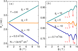
Figure 1: (Color online) The calculated resistivity $R_{xx}$ as a function of the magnetic field $B$ having different effective g-factors: $g_{z}=0,10$ and $-10$ for a TI surface system with electron sheet density $N=1.3\times 10^{12}\,{\rm cm}^{-2}$ in the cases of zero-magnetic-field mobility $\mu=0.2\,{\rm m^{2}/Vs}$ (a) and $\mu=0.7\,{\rm m^{2}/Vs}$ (b). Several integer-number positions of filling factor $\nu=2\pi N/(eB)$ are marked in (b).

Fig. 1 shows the calculated magnetoresistivity $R_{xx}$ versus the magnetic field strength $B$ for a TI surface system with electron sheet density $N=1.3\times 10^{12}\,{\rm cm}^{-2}$ but having different effective g-factors: $g_{z}=0,10$ and $-10$ for two values of zero-magnetic-field mobility $\mu=0.2\,{\rm m^{2}/Vs}$ and $\mu=0.7\,{\rm m^{2}/Vs}$, representing different degree of Landau-level broadening. In the case without Zeeman splitting ($g_{z}=0$) the resistivity $R_{xx}$ exhibits almost no change with changing magnetic field up to 10 T, except the Shubnikov-de Haas (SdH) oscillation showing up in the case of $\mu=0.7\,{\rm m^{2}/Vs}$. This kind of magnetoresistance behavior was indeed seen experimentally in the electron-hole symmetrical massless system of single-layer graphene.tan2011shubnikov In the case of a positive g-factor, $g_{z}=10$, the magnetoresistivity increases linearly with increasing magnetic field; while for a negative g-factor, $g_{z}=-10$, the magnetoresistivity decreases linearly with increasing magnetic field.

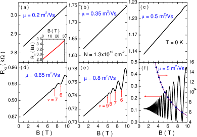
Figure 2: (Color online) The longitudinal resistivity $R_{xx}$ is shown as a function of the magnetic field $B$ for different values of zero-magnetic-field mobility: (a) $\mu=0.2$, (b) $0.35$, (c) $0.5$, (d) $0.65$, (e) $0.8$, and (f) $5\,{\rm m^{2}/Vs}$. The inset of (a) illustrates the same for a larger magnetic-field range $0<B<30\,{\rm T}$. The filling factor $\nu$ is plotted versus the magnetic field in (f); and several integer-number positions of $\nu$ are also marked in (d) and (e). Here the surface electron density $N=1.3\times 10^{12}\,{\rm cm}^{-2}$ and the lattice temperature $T=0\,{\rm K}$.

In the following we will give more detailed examination on the linearly increasing magnetoresistance in the positive $g_{z}$ case.

Fig. 2 shows the calculated resistivity $R_{xx}$ versus the magnetic field strength $B$ at lattice temperature $T=0\,{\rm K}$ for system of carrier sheet density $N=1.3\times 10^{12}\,{\rm cm}^{-2}$ and $g_{z}=10$, having different zero-field mobility $\mu=0.2,0.35,0.5,0.65,0.8$ and $5\,{\rm m^{2}/Vs}$. All resistivity curves for mobility $\mu\leq 0.8\,{\rm m^{2}/Vs}$ exhibit clear linearity in the magnetic-field range and appear no tendency of saturation at the highest field shown in the figure. Especially, for the case $\mu=0.2\,{\rm m^{2}/Vs}$, the linear behavior extends even up to the magnetic field of $30\,{\rm T}$, as illustrated in the inset of Fig. 2(a). This feature contradicts the classical MR which saturates at sufficiently large magnetic field $B\gg\mu^{-1}$.

Note that here we only present the calculated $R_{xx}$ for magnetic field $B$ larger than $B_{c}=1$ T, for which a sufficient energy gap $2|\delta_{z}|=g_{z}\mu_{\rm B}B$ is assumed to open that with further increase of the magnetic field the states in the “+”-branch levels no longer shrink into the zero level and thus it should be excluded from the conduction band. This is of course not true for very weak magnetic field. When $B\rightarrow 0$ the energy gap $2|\delta_{z}|\rightarrow 0$, the situation becomes similar to the case of $g_{z}=0$: the whole upper half of the zero-level states are available to electron occupation and we should have a flat resistivity $R_{xx}$ when changing magnetic field. With increasing $B$ the portion of the zero-level states available to conduction electrons decreases until the magnetic field reaches $B_{c}$. As a result the resistivity $R_{xx}$ should exhibit a crossover from a flat changing at small $B$ to positively linear increasing at $B>B_{c}$. This is just the behavior observed in the TI Bi₂Se₃.Tang2011

Note that in the case of $\mu=0.2\,{\rm m^{2}/Vs}$, the broadened Landau-level widths are always larger than the neighboring level interval: $2{\it\Gamma}\gtrsim\Delta\varepsilon_{n}=\varepsilon_{n+1}-\varepsilon_{n}$, which requires $\mu\lesssim(4e\alpha/N)[(\sqrt{n+1}+\sqrt{n})/\pi]^{2}$, even for the lowest Landau level $n=1$, i.e. the whole Landau-level spectrum is smeared. With increasing the zero-field mobility the magnitude of resistivity $R_{xx}$ decreases, and when the broadened Landau-level width becomes smaller than the neighboring level interval, $2{\it\Gamma}\lesssim\Delta\varepsilon_{n}$, a weak SdH oscillation begin to occur around the linearly-dependent average value of $R_{xx}$ at higher portion of the magnetic field range, as seen in Fig. 2 (c), (d) and (e) for $\mu=0.5,0.65$ and $0.8\,{\rm m^{2}/Vs}$. On the other hand, in the case of large mobility, e.g. $\mu=5\,{\rm m^{2}/Vs}$, where the broadened Landau-level widths $2{\it\Gamma}$ are much smaller than the neighboring level interval even for level index $n$ as large as $30$, the magnetoresistivity shows pronounced SdH oscillation and the linear-dependent behavior disappears, before the appearance of quantum Hall effect,Zheng2002 ; zhang2005experimental ; Gusynin2005 as shown in Fig. 2(f).

Abrikosov’s model for the LMR requires the applied magnetic field large enough to reach the quantum limit at which all the carriers are within the lowest Landau level,Abrikosov1998 while it is obvious that more than one Landau levels are occupied in the experimental samples in the field range in which the linear and non-saturating magnetoresistivity was observed.Tang2011 For the given electron surface density $N=1.3\times 10^{12}\,{\rm cm}^{-2}$, the number of occupied Landau levels, or the filling factor $\nu=2\pi N/(eB)$, at different magnetic fields is shown in Fig. 2(f), as well as in the Fig. 2(d) and (e), where the integer-number positions of ${\nu}$, i.e. filling up to entire $\nu$ Landau levels, coincide with the minima of the density-of-states or the dips of SdH oscillation. This is in contrast with $g_{z}=0$ case, where the integer number of ${\nu}$, which implies a filling up to the center position of the $\nu$th Landau levels, locates at a peak of SdH oscillation, as shown in Fig. 1b. The observed SdH oscillations in the Bi₂Se₃ nanoribbon exhibiting nonsaturating surface LMR in the experimentTang2011 favor the former case: a finite positive effective $g_{z}>0$.

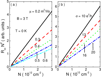
Figure 3: (Color online) $R_{xx}N^{2}$ is plotted as a function of the surface electron density $N$ at magnetic field $B=3\,{\rm T}$: (a) at different values of zero-field mobility $\mu$, and (b) at different values of zero-field conductivity $\sigma$.

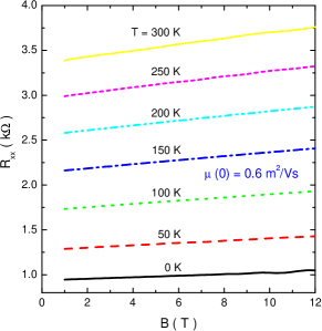
Figure 4: (Color online) The longitudinal resistivity of the surface state of a TI versus magnetic field $B$ at various lattice temperatures. Here the zero-magnetic-field mobility at zero temperature is $\mu(0)=0.6\,{\rm m^{2}/Vs}$.

Next, we examine the density-dependence of the linear magnetoresistivity. To compare with Abrikosov’s quantum magnetoresistance which suggests a $R_{xx}\propto N^{-2}$ behavior,Abrikosov1998 ; Abrikosov2003 we show the calculated $R_{xx}N^{2}$ for above LMR versus the carrier sheet density $N$ in Fig. 3 at fixed magnetic field $B=3$ T. The mobility is taken respectively to be $\mu=0.2,0.3,0.4,0.5$ and $0.6$ m²/Vs to make the resistivity in the LMR regime. A clearly linear dependence of $R_{xx}N^{2}$ on the surface density $N$ is seen in all cases, indicating that this non-saturating linear resistivity is almost inversely proportional to the carrier density. In the figure we also show $R_{xx}N^{2}$ versus $N$ under the condition of different given conductivity $\sigma=Ne\mu=10,13,16$ and $20\,e^{2}/h$. In this case the half-width $\varGamma$ is independent of surface density. The linear dependence still holds, indicating that this linear behavior is not sensitive to the modest $N$-dependence of Landau level broadening $\varGamma$ as long as the system is in the overlapped Landau level regime.

From the above discussion, it is obvious that LMR shows up in the system having overlapped Landau levels and the separation of Landau levels makes the MR departure from the linear increase. At high temperature, the thermal energy would smear the level separation and phonon scatterings further broaden Landau levels. Hence, it is believed that this LMR will be robust against raising temperature. This is indeed the case as seen in Fig. 4, where we plot the calculated magnetoresistivity $R_{xx}$ for the above system with zero-temperature linear mobility $\mu(0)=0.6$ m²/Vs versus the magnetic field at different lattice temperatures. We can see that raising temperature to room temperature has little effect on the linearity of MR. Due to the decreased mobility at higher temperature from phonon scattering, the weak SdH oscillation on the linear background tends to vanish. These features are in good agreement with the experimental report.Tang2011

V summary

In summary, we have studied the two-dimensional magnetotransport in the flat surface of a three-dimensional TI, which arises from the surface states with a wavevector-linear energy dispersion and a finite, positive Zeeman splitting within the bulk energy gap. When the level broadening is comparable to or larger than the Landau-level separation and the conduction electrons spread over many Landau levels, a positive, dominantly linear and non-saturating magnetoresistance appears within a quite wide range of magnetic field and persists up to room temperature. This remarkable LMR provides a possible mechanism for the recently observed linear magnetoresistance in topological insulator Bi₂Se₃ nanoribbons.Tang2011

In contrast to quantum Hall effect which appears in the case of well formed Landau levels and to Abrikosov’s quantum magnetotransport,Abrikosov1998 ; abrikosov2000quantum which is limited to the extreme quantum limit that all electrons coalesce into the lowest Landau level, the discussed LMR is a phenomena of pure classical two-dimensional magnetotransport in a system having linear-energy-dispersion, appearing in the regime of overlapped Landau levels, irrespective of its showing up in relatively high magnetic field range. Furthermore, the present scheme deals with spatially uniform case without invoking the mobility fluctuation in a strongly inhomogeneous system, which is required in the classical Parish and Littlewood model to produce a LMR.Parish2003

The appearance of this significant positive-increasing linear magnetoresistance depends on the existence of a positive and sizable effective g-factor. If the Zeeman energy splitting is quite small the resistivity $R_{xx}$ would exhibit little change with changing magnetic field. In the case of a negative and sizable effective g-factor the magnetoresistivity would decrease linearly with increasing magnetic field. Therefore, the behavior of the longitudinal resistivity versus magnetic field may provide a useful way for judging the direction and the size of the effective Zeeman energy splitting in TI surface states.

References

- (1) R. Xu, A. Husmann, T. F. Rosenbaum, M. L. Saboungi, J. E. Enderby, and P. B. Littlewood, Nature 390, 57 (1997).
- (2) J. Hu and T. Rosenbaum, Nature Mater. 7, 697 (2008).
- (3) M. P. Delmo, S. Yamamoto, S. Kasai, T. Ono, and K. Kobayashi, Nature 457, 1112 (2009).
- (4) H. G. Johnson, S. P. Bennett, R. Barua, L. H. Lewis, and D. Heiman, Phys. Rev. B 82, 085202 (2010).
- (5) A. L. Friedman, J. L. Tedesco, P. M. Campbell, J. C. Culbertson, E. Aifer, F. K. Perkins, R. L. Myers-Ward, J. K. Hite, C. R. Eddy Jr, G. G. Jernigan, and D. K. Gaskill, Nano Lett. 10, 3962 (2010).
- (6) P. L. Kapitza, Proc. R. Soc. A 123, 292 (1929).
- (7) A. A. Abrikosov, Phys. Rev. B 58, 2788 (1998).
- (8) A. A. Abrikosov, Europhys. Lett. 49, 789 (2000).
- (9) M. M. Parish and P. B. Littlewood, Nature 426, 162 (2003).
- (10) C. L. Kane and E. J. Mele, Phys. Rev. Lett. 95, 226801 (2005).
- (11) M. Z. Hasan and C. L. Kane, Rev. Mod. Phys. 82, 3045 (2010).
- (12) X. L. Qi and S. C. Zhang, Rev. Mod. Phys. 83, 1057 (2011).
- (13) Y. Xia, D. Qian, D. Hsieh, L. Wray, A. Pal, H. Lin, A. Bansil, D. Grauer, Y. S. Hor, R. J. Cava, and M. Z. Hasan, Nat. Phys. 5, 398 (2009).
- (14) H. J. Zhang, C. X. Liu, X. L. Qi, X. Dai, Z. Fang and S. C. Zhang, Nat. Phys. 5, 438 (2009).
- (15) C. X. Liu, X. L. Qi, H. J. Zhang, X. Dai, Z. Fang, and S. C. Zhang, Phys. Rev. B 82, 045122 (2010).
- (16) H. Tang, D. Liang, R. L. J. Qiu, and X. P. A. Gao, ACS Nano 5, 7510 (2011).
- (17) X. L. Lei and C. S. Ting, Phys. Rev. B 30, 4809 (1984); Phys. Rev. B 32, 1112 (1985).
- (18) X. L. Lei, J. L. Birman, and C. S. Ting, J. Appl. Phys. 58, 2270 (1985).
- (19) W. Cai, X. L. Lei, and C. S. Ting, Phys. Rev. B 31, 4070 (1985); X. L. Lei, W. Cai, and C. S. Ting, J. Phys. C: Solid State, 18, 4315 (1985).
- (20) C. S. Ting, S. C. Ying, and J. J. Quinn, Phys. Rev. B 16, 5394 (1977).
- (21) J. W. McClure, Phys. Rev. 104, 666 (1956).
- (22) Y. Zheng and T. Ando, Phys. Rev. B 65, 245420 (2002).
- (23) M. Zarea and S. E. Ulloa, Phys. Rev. B 72, 085342 (2005).
- (24) Z. G. Wang, Z. G. Fu, S. X. Wang, and P. Zhang, Phys. Rev. B 82, 085429 (2010).
- (25) A. A. Taskin and Y. Ando, Phys. Rev. B 84, 035301 (2011).
- (26) T. Ando, A. B. Fowler, and F. Stern, Rev. Mod. Phys. 54, 437 (1982).
- (27) X. L. Lei and S. Y. Liu, Phys. Rev. Lett. 91, 226805 (2003).
- (28) C. M. Wang and F. J. Yu, Phys. Rev. B 84, 155440 (2011).
- (29) D. Culcer, E. H. Hwang, T. D. Stanescu, and S. Das Sarma, Phys. Rev. B 82, 155457 (2010).
- (30) O. Madelung, Semiconductors: Data Handbook (Springer Verlag, 2004).
- (31) X. Zhu, L. Santos, R. Sankar, S. Chikara, C. . Howard, F. C. Chou, C. Chamon, and M. El-Batanouny, Phys. Rev. Lett. 107, 186102 (2011).
- (32) Z. B. Tan, C. L. Tan, L. Ma, G. T. Liu, L. Lu, and C. L. Yang, Phys. Rev. B 84, 115429 (2011).
- (33) Y. Zhang, Y. Tan, H. Stormer, and P. Kim, Nature 438, 201 (2005).
- (34) V. P. Gusynin and S. G. Sharapov, Phys. Rev. Lett. 95, 146801 (2005).
- (35) A. A. Abrikosov, J. Phys. A: Math. Gen. 36, 9119 (2003).