Signalling noise enhances chemotactic drift of E. coli

Abstract

Noise in transduction of chemotactic stimuli to the flagellar motor of E. coli will affect the random run-and-tumble motion of the cell and the ability to perform chemotaxis. Here we use numerical simulations to show that an intermediate level of noise in the slow methylation dynamics enhances drift while not compromising localisation near concentration peaks. A minimal model shows how such an optimal noise level arises from the interplay of noise and the dependence of the motor response on the network output. Our results suggest that cells can exploit noise to improve chemotactic performance.

The motion of Escherichia coli consists of a series of “runs”, where the cell swims in a roughly constant direction, and “tumbles”, during which the cell randomly reorients Berg72 . In a spatially-varying environment the bacterium performs chemotaxis by biasing this random motion in the direction of favourable conditions. A well-studied signalling cascade Berg_book detects environmental ligand stimuli and regulates the stochastic switching of the rotary flagellar motors between counter-clockwise (run) and clockwise (tumble) rotation Berg72 . However, the biochemical reactions making up this signalling pathway are inherently random events, and the noise introduced to the signal in this way will affect the swimming behaviour and ability of a cell to respond to gradient stimuli. Here we show how signalling noise can be beneficial for chemotactic performance.

Chemoattractant stimuli are detected by the binding of ligands to membrane receptor complexes, which suppresses the activity of the receptor-associated kinase CheA. Consequently, the phosphorylation level of the response regulator CheY, which in its phosphorylated form (CheYp) binds to the flagellar motor and promotes tumbling, decreases leading to longer runs. Conversely, a reduction in ligand binding leads to an increase in CheYp and shorter runs. Hence, the random walk motion of the bacterium is biased in the direction of increasing chemoattractant concentration. Crucially, the chemotaxis network also includes a negative feedback from CheA activity to receptor methylation. This ensures adaptation of the network response to constant stimuli, enabling the network to detect temporal derivatives of the observed ligand signal Segall86 and allowing sensitivity to a wide range of ligand concentrations Sourjik02 .

Receptor methylation and demethylation reactions are a significant source of noise in the signalling network Korobkova04 , because (i) the timescale of methylation ($\sim 10s$ Shimizu10 ) is much longer than the other timescales in the network (ligand-receptor binding and receptor activity changes: $\sim 1ms$; CheY phosphorylation and motor switching: $\lesssim 1s$), meaning that the downstream network cannot integrate out slow methylation fluctuations; and (ii) methylation occurs at a small number of sites on each receptor catalysed by a small number of the enzymes CheR and CheB, meaning that small-number fluctuations in the overall methylation level can be significant. Importantly, the output of the noisy signalling network also affects the ligand signal experienced by the cell via modulation of the tumbling dynamics and hence the swimming trajectory. This highly non-linear feedback potentially means that noise may significantly affect the chemotactic response.

Previous studies have shown that, in the absence of chemoattractant gradients, noise in (de)methylation reactions can lead to a power-law distribution of run durations Korobkova04 ; Tu05 . The resulting super-diffusive motion may enhance search efficiency compared to Brownian motion Korobkova04 ; Matthaus09 . It has also recently been shown that slow fluctuations in the methylation dynamics can allow for enhancement of drift in linear gradients Matthaus09 ; Emonet08 at the expense of the ability of cells to localise in regions of high ligand concentration Matthaus09 . However, the mechanism by which noise enhances drift remains unclear.

In this paper we study the effects of receptor (de)methylation noise on chemotactic performance. We show that below a threshold noise level the steady-state performance of cells in a sinusoidal ligand field does not improve as noise is reduced. We also find that an optimal noise level, comparable to this noise threshold, maximises the drift velocity in exponential gradients. Analytic approximations of a minimal model reveal that in the relevant regime where motor switching is fast compared to adaptation, drift enhancement results from the interplay of noise with the response of the motor switching rate to the output of the signalling network.

To study the effects of signalling noise on the chemotactic behaviour of E. coli we performed simulations of bacterial populations using a scheme coupling swimming and signalling Jiang10 . Signalling dynamics are simulated according to a recently-developed model Tu08 ; Shimizu10 describing the CheA activity, receptor methylation level, and phosphorylated CheYp level. The stochastic switching of the two-state motor with CheYp-dependent switching rates, and the run-and-tumble dynamics of the bacterium in a three-dimensional environment are also simulated. Noise was introduced into the deterministic model considered in Jiang10 by adding a Gaussian white noise source to the dynamics of methylation. The strength of this noise is proportional to a parameter $\gamma^{-1}$ which is used to control the impact of noise without changing the response time of the network (full details of the model can be found in the Supplementary Information).

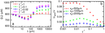
Figure 1: (a) Mean steady-state ligand level $\langle{[L]}\rangle$ for a population of cells in a sinusoidal ligand profile with $[L_{0}]=800\mu M$ and $A=0.25$, for different noise strengths $\gamma^{-1}$. Dotted lines show the maximal and minimal concentrations at $[L]=[L_{0}](1\pm A)$. For short wavelengths $\lambda\lesssim 150\mu{m}$ chemotactic cells perform worse than a simple random walk, for which $\langle{[L]}\rangle=[L_{0}]$ (dashed line). Increasing the noise reduces the ability of cells to localise in regions of high ligand concentration. (b) Transient drift velocity in an exponential ligand profile, with $[L_{0}]=20\mu M$ as the noise strength $\gamma^{-1}$ is varied. In shallow gradients $x_{0}>500\mu{m}$ drift is fastest at intermediate noise strengths.

We first considered the ability of cells to localise in the vicinity of ligand concentration peaks by studying the steady-state distribution of cells in a sinusoidally-varying ligand profile, $[L(\mathbf{x})]=[L_{0}](1+A\cos 2\pi x/\lambda)$. Figure 1a shows the average ligand level $\langle{[L]}\rangle=N_{\rm cells}^{-1}\sum_{i\in{\rm cells}}[L({\mathbf{x}}_{i})]$ experienced by the simulated population as the gradient length-scale $\lambda$ and noise strength $\gamma^{-1}$ are varied. Non-chemotactic cells performing an unbiased random walk would have $\langle{[L]}\rangle=[L_{0}]$. We first consider cells with deterministic signalling, $\gamma^{-1}\to 0$; the trajectories of such cells are still noisy since motor switching and reorientation angles during tumbles remain stochastic. For gradient length scales shorter than the typical run length of unstimulated cells, $\lambda\lesssim 5\mu{m}$, cells are unable to react to the extremely rapidly changing ligand level and effectively perform an unbiased random walk. For long length scales $\lambda\gtrsim 200\mu{m}$ cells are able to reliably localise in the vicinity of ligand concentration maxima. However, in an intermediate range of length scales we find that $\langle{[L]}\rangle<[L_{0}]$. Here, methylation is too slow to keep the CheYp level in the sensitive range of the motor as cells run in directions of increasing ligand, and as a result cells repeatedly overshoot ligand concentration peaks, an extreme example of the ‘volcano effect’ which has been observed previously Bray07 .

The shape of $\langle{[L]}\rangle$ as a function of $\lambda$ is largely unchanged as the methylation noise strength $\gamma^{-1}$ is increased; however, the difference between $\langle{[L]}\rangle$ and $[L_{0}]$ at a given $\lambda$ is decreased. Noise moves cells away from concentration maxima when $\lambda$ is large, but also out of minima when $\lambda\lesssim 200\mu{m}$. However, since chemotaxis remains detrimental in rapidly-varying profiles, it appears unlikely that signalling is optimised for this type of environment. We therefore focus on the regime of long wavelengths. Importantly, here we find that there is an effective noise threshold around $\gamma^{-1}\sim 0.01$; provided signalling noise is kept below this level, it is not detrimental for localisation near ligand maxima, which is instead limited by the intrinsically random run-and-tumble motion of the cell.

Noise reduction in biochemical signalling is typically energetically costly, requiring for example increased protein production or more rapid turn-over. Our observation of a noise threshold suggests that there is no benefit, at least in terms of localisation performance, to reducing noise below this level. Moreover, it raises the possibility that this noise could somehow be exploited by the cell. Bacterial chemotaxis has two conflicting goals Clark05 : localisation in regions of high chemoattractant, and rapid drift in favourable directions. The observed chemotactic response has been interpreted as a compromise between these two objectives Clark05 ; Celani10 . It is therefore important to also consider the effects of noise on the transient drift rate of cells.

We therefore investigated transient chemotactic drift in an exponential ligand gradient, $[L(\mathbf{x})]=[L_{0}]\exp(x/x_{0})$. Figure 1b shows the drift velocity, estimated from the linear regime of the mean $x$-position $\langle{x(t)}\rangle=N_{\rm cells}^{-1}\sum_{i\in{\rm cells}}x_{i}(t)$ as a function of elapsed time, for a population initially located at $\mathbf{x}=\vec{0}$. We considered only shallow gradients, $x_{0}\geq 500\mu{m}$, for which $\langle{x(t)}\rangle$ reaches a stable constant drift regime before saturation of ligand binding. Based on experimentally-observed ramp responses Shimizu10 , cells are expected to be sensitive to gradients with $x_{0}$ beyond $10000\mu m$. Interestingly, we see that the drift velocity has a non-monotonic dependence on methylation noise strength: drift in a cell with noisy methylation dynamics can be faster than in cells with no methylation noise, and there is a steepness-dependent noise strength that maximises the drift velocity. This effect is also observed taking other measures of drift performance such as the maximal drift velocity or the mean position of the population after some fixed time. Our results are consistent with previous reports that cells with signalling noise drift more rapidly in linear gradients Matthaus09 ; Emonet08 . We note that the optimal noise strength $\gamma^{-1}\approx 0.01-0.02$ gives rise to a coefficient of variation in the CheYp level of around $0.2$, comparable to the variability required Tu05 to reproduce the experimentally-observed power law run-time distribution Korobkova04 . Importantly, we also see that at the optimal noise level neither the drift velocity in steep gradients nor the steady-state localisation performance of cells is significantly compromised.

To understand the origin of this noise-induced drift enhancement in shallow gradients we studied a minimal model of chemotactic drift, shown in Fig. 2a (see the Supplementary Information for derivation). We consider motion in one spatial dimension; cells can be in two states, ‘$+$’ or ‘$-$’, which correspond to motion with velocity $\tilde{v}=\pm 1$ in directions of increasing or decreasing ligand concentration respectively. We assume that directional changes are instantaneous and hence no tumbling state is considered. Furthermore we assume that the CheYp level simply tracks CheA activity, such that the internal dynamics of the signalling pathway can be represented by a single state variable, $\delta a(t)$, that represents the deviation of the pathway activity from its adapted value (but with the direction of action of the gradient reversed) and evolves according to $\dot{\delta a}=\tilde{v}r-\delta a+\sigma\Gamma(t)$. Here $r$ represents the stimulus from the ligand gradient, $\sigma$ is the strength of methylation noise, and $\Gamma(t)$ is a Gaussian white noise process with unit variance. We take $r$ to be a constant since in the full chemotaxis network the effective stimulus strength goes as $\partial_{x}{\log[L(x)]}\sim x_{0}^{-1}$ for an exponential gradient. Since the noise-enhancement of drift is observed in shallow gradients we focus on the regime of small $r<1$, a range of stimuli comparable in the rescaled parameter space to the gradients for which drift enhancement is observed in the full model. Finally, the switching propensity between ‘$+$’ and ‘$-$’ states is given by $\omega(\delta a)=\kappa(1-\delta a)$ for $\delta a\leq 1$ and $\omega(\delta a)=0$ otherwise. This form for $\omega$ approximates the highly non-linear dependence of the motor switching propensity on the CheYp level Cluzel00 with $\kappa$ setting the typical rate of reorientations relative to adaptation, and is chosen for computational simplicity. However, similar results are observed with $\omega$ a smooth decreasing function of $\delta a$. Following Erban04 , evolution equations can be written for the joint probability $p_{\pm}(\delta a;t)$ of a cell to be in the ‘$+$’ or ‘$-$’ state with internal variable $\delta a$,

$$\partial_{t}{p_{\pm}}-\partial_{\delta a}{\left[\left(\delta a\mp r\right)p_{\pm}\right]}=\frac{\sigma^{2}}{2}\partial_{\delta a}^{2}{p_{\pm}}\mp\omega(\delta a)(p_{+}-p_{-})$$ (1)

where the first term on the right-hand side of Eq. 1 is due to the noise in the dynamics of $\delta a$. Thus in each state, cells effectively diffuse in a potential $V_{\pm}(\delta a)\sim(\delta a\mp r)^{2}$ with diffusion constant $\sigma^{2}/2$. The net population drift velocity in this minimal model is given simply by $\langle{J(t)}\rangle=\int_{-\infty}^{\infty}\left[p_{+}(\delta a;t)-p_{-}(\delta a;t)\right]d\delta a$.

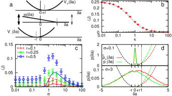
Figure 2: (a) Schematic depiction of the minimal model. Cells switch between the two states ‘$+$’ and ‘$-$’ with rate $\omega(\delta a)$. The internal coordinate $\delta a$ diffuses within the potential $V_{\pm}(\delta a)$. (b) Steady-state drift $\langle{J}\rangle$ as switching rate $\kappa$ is varied, for $r=0.25$ and $\sigma=0$. Points show simulation results; dashed line shows $\langle{J}\rangle=r/(1+2\kappa)$. (c) Steady-state drift $\langle{J}\rangle$ as the noise strength $\sigma$ is varied for different stimulus strengths $r$, with $\kappa=10$. For small $r$, $\langle{J}\rangle$ is maximised for $\sigma>0$. Lines show the approximate results for $\kappa\to\infty$, Eq. 3. (d) Probability densities $p_{\pm}(\delta a)$ (solid lines) when $r=0.5$, with $\kappa=10$. For small $\sigma$, $p_{\pm}(\delta a)$ are similar and peaked around $\delta a=0$. For larger $\sigma$, the different forces experienced when $\omega(\delta a)$ is small lead to differences between the distributions $p_{\pm}(\delta a)$. Dashed lines show the effective potentials $V_{\rm eff}(\delta a<1)$ and $V_{\pm}(\delta a>1)$.

In the absence of noise, $\sigma=0$, Eq. 1 can be solved to find the steady-state drift. While the full expression is uninformative (see Supplementary Information), for small $r\ll 1$ it can be approximated as $\langle{J}\rangle\approx r/(1+2\kappa)$ (see Fig. 2b). We see that increasing $\kappa$ decreases $\langle{J}\rangle$, a result that also holds when $\sigma>0$; intuitively, if the typical run duration is shorter, less information can be extracted about the current direction during a single run, and hence the reliability with which the tumbling propensity can be regulated is reduced.

An exact solution to Eq. 1 when $\sigma>0$ is less straightforward. Since in the full chemotaxis network the typical switching rate is fast compared to the adaptation time, with an effective value of $\kappa\approx 10$, we focus in the remainder of the paper on the regime $\kappa\gg 1$ for which both numerical solutions and an analytic limit solution are possible. Figure 2c shows the numerically-evaluated $\langle{J}\rangle$ at $\kappa=10$ as the noise $\sigma$ is varied for different stimulus strengths $r$. We can see that the minimal model qualitatively reproduces the results of the full model for shallow gradients, with $\langle{J}\rangle$ showing a maximum at $\sigma\gtrsim 1$.

To understand the origin of this noise-induced maximum it is useful to consider the limit of rapid switching, $\kappa\to\infty$. In the region $\delta a<1$, cells rapidly exchange between ‘$+$’ and ‘$-$’ states, such that $p_{+}(\delta a)=p_{-}(\delta a)$. In this region, therefore, cells spend equal time in each of the two states while moving in the effective mixed potential $V_{\rm eff}(\delta a)=[V_{+}(\delta a)+V_{-}(\delta a)]/2\sim(\delta a^{2}+r^{2})$. However, any cell which crosses into the region $\delta a>1$, where $\omega(\delta a)=0$, will experience only the potential associated with its current state, $V_{\pm}(\delta a)$, until returning to the boundary $\delta a=1$. The average net drift can be calculated in terms of the mean time spent in each region, $\delta a<1$ and $\delta a>1$ in either the ‘$+$’ and ‘$-$’ states as

$$\langle{J}\rangle=\frac{T^{\delta a>1}_{+}-T^{\delta a>1}_{-}}{T^{\delta a>1}_{+}+2T^{\delta a<1}+T^{\delta a>1}_{-}}$$ (2)

where $T^{\delta a<1}$ is the typical time spent in the region $\delta a<1$ accounting for both the ‘$+$’ and ‘$-$’ states and we have used the fact that these cells have no bias in their direction. Evaluating the typical times spent diffusing in the appropriate potentials we find

$$\langle{J}\rangle\approx r\left[\frac{\exp({\sigma^{-2}})}{\sqrt{\pi\sigma^{2}}}-\frac{{\rm erfc}{(\sigma^{-1})}}{\sigma^{2}}\right],$$ (3)

which can be seen to have a maximum at $\sigma\approx 2$ (Fig. 2c, see Supplementary Information for an exact expression and full derivation).

When the noise level is small, $\sigma<1$, cells occupy the minimum of $V_{\rm eff}(\delta a)$ at $\delta a=0$ and $p_{+}(\delta a)\approx p_{-}(\delta a)$ (see Fig. 2d), such that the net drift $\langle{J}\rangle\approx 0$. As the noise is increased, so too is the rate at which cells reach the transition point $\delta a=1$, beyond which $\omega(\delta a)=0$. Importantly, the offset between the minima of $V_{+}(\delta a)$ and $V_{-}(\delta a)$ means that cells in the region $\delta a>1$ in the ‘$-$’ state will experience a stronger force in the $-\delta a$-direction than cells in the ‘$+$’ state, $\lvert{\partial_{\delta a}{V_{+}}}\rvert<\lvert{\partial_{\delta a}{V_{-}}}\rvert$. Hence the mean time spent diffusing in the region $\delta a>1$ before returning to the boundary at $\delta a=1$ will be longer in the ‘$+$’ state than in the ‘$-$’ state, $T^{\delta a>1}_{+}>T^{\delta a>1}_{-}$. This is the origin of the drift enhancement by noise: as $\sigma$ is increased beyond unity, cells spend an increasing amount of time in the region $\delta a>1$, and so the magnitude of this effect and hence the drift $\langle{J}\rangle$ increase. For even larger values of the noise, the difference in the amount of time spent in the ‘$+$’ and ‘$-$’ states decreases again, because now diffusion dominates over the difference in forces. Hence $\langle{J}\rangle$ decreases again for $\sigma\gg 1$.

While Fig. 2c shows qualitative agreement between Eq. 3 and the numerical results for $\kappa=10$, $\langle{J}\rangle$ calculated for $\kappa\to\infty$ underestimates the drift when $\kappa$ is finite (see also Supplementary Information). With a finite switching rate, $p_{\pm}(\delta a<1)$ need not be precisely identical; indeed, an effective positive feedback acts on differences between $p_{\pm}(\delta a<1)$ due to the variation of $\omega(\delta a)$ with $\delta a<1$. As $\delta a$ becomes larger and $\omega(\delta a)$ decreases, cells will spend more time in the potential $V_{\pm}(\delta a)$. Since cells in the ‘$+$’ state tend to drift towards larger values of $\delta a$ than cells in the ‘$-$’ state, cells will typically remain in the ‘$+$’ state for longer, allowing for further drift and amplifying the differences between $p_{+}(\delta a)$ and $p_{-}(\delta a)$. This means that (i) cells with $\delta a<1$ also contribute positively to $\langle{J}\rangle$; and (ii) more cells enter the region $\delta a>1$ in the ‘$+$’ than the ‘$-$’ state, further increasing $\langle{J}\rangle$.

The maximal drift at the optimal noise strength for large $\kappa\gg 1$ remains less than $r$, the drift which is achieved for small $\kappa\to 0$ and $\sigma\to 0$ (see Fig. 2b), suggesting the E. coli could instead enhance chemotactic performance simply by reducing the switching rate and signalling noise. However, chemotactic performance also depends on steady-state localization. This motivated us to study the effects of varying the rate of motor switching in the full model. As shown in Fig. 3, reducing the switching rate increases the transient drift velocity at low noise levels, but this is accompanied by a decrease in steady-state performance. This data emphasises that the choice of chemotactic network parameters entails a trade-off between steady-state and transient performance. The switching rate cannot be significantly decreased without severely compromising steady-state performance. But at the switching rates observed in real cells, a moderate level of noise improves drift performance compared to a system without noise, without harming steady-state localisation and additionally reducing the cost of signalling.

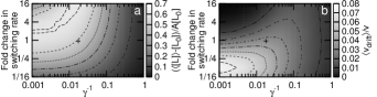
Figure 3: Effects of varying the noise strength $\gamma^{-1}$ and typical rate of motor switching in the full model on (a) steady-state ($\lambda=500\mu m$), and (b) transient ($x_{0}=1000\mu m$) chemotactic performance. At intermediate switching rates, the optimal drift velocity can be achieved with a finite noise level without compromising steady-state performance. The estimated wild-type parameters are indicted with $+$.

The principal result of our manuscript is an explanation of the mechanism by which noise can enhance chemotactic drift. This mechanism is unlike the noise-driven motion of Brownian ratchets or motors Reimann02 in that drift reflects differences in the mean occupancy of internal states of the system, rather than motion in an underlying spatial potential. The effect described here can potentially enhance the bias of any two-state system in which the rate of switching between these states is dependent on internal variables of the system and is fast compared to the relaxation in either state. The essence of the mechanism is that the fast switching obscures the difference between the two states, unless noise is sufficiently strong that the system transiently passes into a regime of slow switching. Then the asymmetry between the two states is felt, and a bias is induced in the steady-state occupancy of the states. This effect also differs from stochastic resonance Gammaitoni98 since it is the enhancement by noise of a steady-state response to a constant input, rather than the enhancement of a dynamic response to a time-varying external signal.

Additionally, we have seen that a finite level of signalling noise can enhance transient chemotactic drift in shallow gradients while not significantly compromising drift in steep gradients or the ability to localise near concentration peaks. More generally, our results suggest that cells may be able to exploit intracellular signalling noise to improve behavioural responses.

I Supplementary Information for “Signalling noise enhances chemotactic drift of E. coli”

II Description of the full chemotaxis model

Here we outline the full model of the chemotaxis pathway, adapted from Jiang10 , used in the simulations. Parameter values used in the simulations are listed in Table S1.

It is assumed that the probability that a given receptor complex is in the active state is in quasi equilibrium and is given by

$$a=\frac{1}{1+\exp(N\epsilon(m,[L]))},$$ (S1)

where $\epsilon$ is the free-energy difference between the active and inactive states and $N$ is the number of responding receptor dimers. The free energy $\epsilon(m,[L])=f_{m}(m)+f_{[L]}([L])$ is a sum of contributions dependent on the receptor methylation state $f_{m}(m)={\alpha}(m_{0}-m)$ and the ligand concentration $f_{[L]}([L])=-\log\left(\frac{1+[L]/K_{A}}{1+[L]/K_{I}}\right)$, where $K_{A}$ and $K_{I}$ are the dissociation constants of ligand to the active and inactive receptors respectively, and roughly define the range of ligand concentrations to which the cell can adapt.

The dynamics governing receptor methylation and demethylation is given by the stochastic equation

$$\frac{d{m}}{d{t}}=k_{R}(1-a)-k_{B}a+\eta(t).$$ (S2)

Here we have introduced the Langevin noise term $\eta(t)$ to represent noise in receptor (de)methylation reactions, with $\langle{\eta}\rangle=0$ and $\langle{\eta(t)\eta(t^{\prime})}\rangle=\gamma^{-1}(k_{R}(1-\overline{a})+k_{B}\overline{a})\delta(t-t^{\prime})$. The values of the rate parameters $k_{R}$ and $k_{B}$ are set from the experimental measurements Shimizu10 of the adapted kinase activity $\overline{a}=k_{R}/(k_{R}+k_{B})=0.5$ (we shall henceforth denote values of the signalling variable in the adapted state with an overbar) and the slope of the feedback transfer function $\{\frac{d{}}{d{a}}(\frac{d{m}}{d{t}})\}_{a=\overline{a}}\approx-(k_{R}+k_{B})=-0.03s^{-1}$. Since the noise $\eta(t)$ is purely additive it does not alter the response time of $m(t)$, which is set by $k_{R}$ and $k_{B}$. The parameter $\gamma^{-1}$ is expected to scale with the number or receptor clusters as $N_{\rm rec}^{-1}$ Emonet08 , while the precise value of $\gamma^{-1}$ will also depend on the cell volume and non-diffusive transport rates of CheR and CheB enzymes.

To propagate the noise from receptor modification, we include explicitly the dynamics for the fraction of CheY which is phosphorylated, $y_{p}$,

$$\frac{d{y_{p}}}{d{t}}=k_{Y}a(1-y_{p})-k_{Z}y_{p},$$ (S3)

Here the first term represents the phosphorylation of CheY by active receptor-CheA complexes, and the second term accounts for dephosphorylation of CheYp by the phosphatase CheZ. The fraction of CheY which is phophorylated in adapted cells is $\overline{y_{p}}=k_{Y}\overline{a}/(k_{Y}\overline{a}+k_{Z})\approx 0.3$ Alon98 . Note that we do not introduce an additional source of noise from the CheYp (de)phosphorylation reactions. This is because we expect such fluctuations to be fast compared to methylation noise, and of small amplitude due to the relatively high copy numbers of CheY and CheZ, and hence to have a small impact on swimming behaviour.

Parameter	Value	Source
$N$	6	Jiang10
$\alpha$	1.7	Jiang10
$m_{0}$	1	Jiang10
$K_{A}$	$3000\mu M$	Jiang10
$K_{I}$	$18.2\mu M$	Jiang10
$\overline{a}$	0.5	Shimizu10
$k_{R}$	$0.015\mbox{s}^{-1}$	Shimizu10
$k_{B}$	$0.015\mbox{s}^{-1}$	Shimizu10
$\overline{y_{p}}$	0.3	Alon98
$k_{Z}$	$2\mbox{s}^{-1}$	Tu08
$k_{Y}$	$1.7\mbox{s}^{-1}$	calculated
$\overline{b}$	$0.25$	Segall86
${\tau}_{0}$	0.2 s	Jiang10 ; Alon98
$H$	10	Jiang10 ; Cluzel00
$\beta$	$282250s^{-1}$	calculated
$D_{\theta}$	$0.123{\rm rad}^{2}s^{-1}$	Jiang10 ; Berg_book
$v$	$16.5\mu{m}s^{-1}$	Jiang10 ; Alon98

Table S1: Parameter values

The tumbling bias is a sigmoidal function of $y_{p}$ with a Hill coefficient $H\approx 10$ Cluzel00 . CheYp modulates only the probability of the motor to switch from counter-clockwise to clockwise rotation, and does not affect the rate of the reverse transition Alon98 . Hence the propensities for a cell to switch from running to tumbling and vice versa are given by Jiang10 ,

$$\omega_{r\rightarrow t}(y_{p})=\beta y_{p}^{H},\ \ \omega_{t\rightarrow r}=\tau^{-1},$$ (S4)

where $\tau$ is the average duration of a tumbling event, which is independent of $y_{p}$. The constant $\beta$ is set such that the clockwise bias in the adapted state is $\overline{b}=\omega_{r\rightarrow t}(\overline{y_{p}})/(\omega_{r\rightarrow t}(\overline{y_{p}})+\omega_{t\rightarrow r})=0.25$ Segall86 . Upon switching from tumbling to running, a new orientation for the cell is chosen randomly and independently of the previous run direction. Introducing correlations between the directions of consecutive runs, as has been observed experimentally Berg72 , does not significantly affect our results.

Simulations are initialised with a population of 10000 cells located at $\mathbf{x}=\vec{0}$ adapted to the local environment. Each cell initially has a random orientation and motor state chosen according to the adapted tumbling bias, $\overline{b}$. In a simulation step of length $\delta t$, running cells move a distance $\delta t\cdot v$ in the direction of their current orientation, where the swimming speed $v$ is taken to be constant; tumbling cells do not move. During runs, the run direction is also perturbed by rotational diffusion with diffusion constant $D_{\theta}$; a random angular displacement is added to the orientation at each time step to account for this. The internal state is also updated according to equations (S1-S3), and the motor state switches with probability $\delta t\cdot\omega_{r\rightarrow t}$ or $\delta t\cdot\omega_{t\rightarrow r}$, given by Eq. S4, as appropriate.

III Derivation of the minimal model

Here we present the complete derivation of the minimal model and its parameters in terms of those of the full model.

We start by considering the internal dynamics of the activity $a$. Taking the time-derivative of Eq. S1 and substituting in Eq. S2 gives

$$\frac{d{a}}{d{t}}=\frac{\partial{a}}{\partial{m}}\frac{d{m}}{d{t}}+\frac{\partial{a}}{\partial{[L]}}\frac{d{[L]}}{d{t}}=Na(1-a)\left[\alpha(k_{R}(1-a)-k_{B}a+\eta)+\frac{K_{I}-K_{A}}{([L]+K_{A})([L]+K_{I})}\frac{\partial{[L]}}{\partial{t}}\right].$$ (S5)

Making the approximation $K_{I}\ll[L]\ll K_{A}$, and using the identity $\overline{a}=k_{R}/(k_{R}+k_{B})$, this expression simplifies to

$$\frac{d{a}}{d{t}}=Na(1-a)\left[\frac{\alpha k_{R}}{\overline{a}}(\overline{a}-a)+\alpha\eta-\frac{1}{[L]}\frac{d{[L]}}{d{t}}\right].$$ (S6)

To model the reduced swimming dynamics in one spatial dimension we write $\frac{d{[L]}}{d{t}}=\pm v\frac{d{[L]}}{d{x}}|_{\rm eff}$, where $|_{\rm eff}$ denotes an effective steepness calculated by integrating $\lvert{\frac{d{[L]}}{d{x}}}\rvert$ over a uniform distribution of run angles in three-dimensional space. For an exponential gradient $[L(\mathbf{x})]=[L_{0}]\exp(x/x_{0})$ we therefore have

$$\frac{d{a}}{d{t}}=Na(1-a)\left[\frac{\alpha k_{R}}{\overline{a}}(\overline{a}-a)+\alpha\eta\mp\frac{v}{2x_{0}}\right].$$ (S7)

Turning to the switching dynamics, we first neglect the presence of the tumbling state since tumbling events are relatively short compared to runs. Then the rate of changing direction is simply given by $\omega(y_{p})=\omega_{r\to t}(y_{p})/2$, where the factor of $1/2$ appears because only half of tumbling events will lead to a change of direction. Next we make a quasi-steady-state assumption that, since the dynamics of $y_{p}(t)$ is fast compared to $a(t)$, $y_{p}(t)=a(t)/\left[a(t)+k_{Z}/k_{Y}\right]$. Substituting into $\omega(y_{p})$ and linearizing about the adapted value $\overline{a}$ leads to

$$\omega(a)\approx\frac{\beta\overline{y_{p}}^{H}}{2}\left[1-(\overline{a}-a)\frac{Hk_{Z}}{\overline{a}(k_{Y}\overline{a}+k_{Z})}\right].$$ (S8)

We define the displacement variable $\delta a$ according to Eq. S8 such that $\omega(\delta a)=\beta\overline{y_{p}}^{H}(1-\delta a)/2$. Next we substitute the corresponding expression for $a(t)$ into Eq. S7 and rescale the units of time according to $\tilde{t}=tN\alpha k_{R}(1-\overline{a})$. Finally, assuming that the noise and stimulus terms as small deviations of the same order as $\delta a$ and retaining only first-order terms in $\delta a$ yields

$$\frac{d{\delta a}}{d{\tilde{t}}}=\pm\frac{vHk_{Z}}{2\alpha k_{R}(k_{Y}\overline{a}+k_{Z})x_{0}}-\delta a+\frac{Hk_{Z}}{k_{R}(k_{Y}\overline{a}+k_{Z})}\eta.$$ (S9)

We identify the first term with $\tilde{v}r$ and the rescaled velocity $\tilde{v}=\pm 1$, such that for a given value of $r$ the equivalent value of $x_{0}$ using the parameters of Table S1 is $x_{0}\approx 2200\mu{m}/r$. Similarly, we can use the expression for the methylation noise strength in the full model to identify

$$\sigma=\frac{Hk_{Z}}{k_{Y}\overline{a}+k_{Z}}\sqrt{\frac{2(1-\overline{a})}{\gamma k_{R}}}\approx 57\gamma^{-1/2}.$$ (S10)

With these parameters, the stimuli in the $r<1$ regime of the minimal model are comparable to gradients in the range for which non-monotonicity in the drift velocity is observed in the full model. The optimal noise level in the minimal models is somewhat smaller than for the full model ($\sigma\approx 2$ is equivalent to $\gamma^{-1}\approx 0.0012$), suggesting that the linear form of $\omega(\delta a)$, which decreases more rapidly than $\omega_{r\to t}$, leads to a slight overestimate of the effect of noise.

It remains only to convert the mean switching rate into the rescaled time units, $\kappa=\frac{\beta\overline{y_{p}}^{H}}{2N\alpha k_{R}(1-\overline{a})}\approx 10$.

IV Exact solution for $\sigma=0$

The full solution of the minimal model in the absence of noise is

$$\langle{J}\rangle=\begin{cases}1-(1-r)\frac{{}_{1}{\rm F}_{1}\left(\kappa(1+r),1+2\kappa;-4r\kappa\right)}{{}_{1}{\rm F}_{1}\left(\kappa(1+r),2\kappa;-4r\kappa\right)}&r<1\\ 1&r\geq 1\end{cases},$$ (S11)

where ${}_{1}{\rm F}_{1}(c_{1},c_{2};x)$ is a Kummer hypergeometric function.

V Exact solution for $\kappa\to\infty$

The exact solution to the minimal model in the limit $\kappa\to\infty$ can be expressed in terms of the typical time spent in the domains $\delta a<1$, and $\delta a>1$ in the ‘$+$’ and ‘$-$’ states, according to

$$\langle{J}\rangle=\frac{T^{\delta a>1}_{+}-T^{\delta a>1}_{-}}{T^{\delta a>1}_{+}+2T^{\delta a<1}+T^{\delta a>1}_{-}}.$$ (S12)

To determine the typical time spent in the region $\delta a<1$, diffusing in the potential $V_{\rm eff}(\delta a)=(\delta a^{2}+r^{2})/2$, before reaching the boundary at $\delta a=1$ we calculate the mean first-passage time from a position $\delta a=1-\varepsilon$, where $\varepsilon$ is a small displacement, to $\delta a=1$, using the standard result Gardiner_book

$$T^{\delta a<1} =\frac{2}{\sigma^{2}}\int_{1-\varepsilon}^{1}dx\ e^{2V_{\rm eff}(x)/\sigma^{2}}\int_{-\infty}^{x}dy\ e^{-2V_{\rm eff}(y)/\sigma^{2}}$$ (S13)

$$\xrightarrow{\varepsilon\to 0}\varepsilon\sqrt{\frac{\pi}{\sigma^{2}}}e^{1/\sigma^{2}}\left(1+{\rm erf}\frac{1}{\sigma}\right),$$ (S14)

where we have used the fact that the diffusion constant in the $\delta a$-coordinate is $\sigma^{2}/2$. Similarly, the time spent in the $\delta a>1$ region starting from a position $\delta a=1+\varepsilon$ can be calculated using the potentials $V_{+}(\delta a)=(\delta a-r)^{2}/2+r$,

$$T_{+}^{\delta a>1} =\frac{2}{\sigma^{2}}\int_{1}^{1+\varepsilon}dx\ e^{2V_{+}(x)/\sigma^{2}}\int_{x}^{\infty}dy\ e^{-2V_{+}(y)/\sigma^{2}}$$ (S15)

$$\xrightarrow{\varepsilon\to 0}\varepsilon\sqrt{\frac{\pi}{\sigma^{2}}}e^{(1-r)^{2}/\sigma^{2}}{\rm erfc}\frac{1-r}{\sigma},$$ (S16)

and $V_{-}(\delta a)=(\delta a+r)^{2}/2-r$,

$$T_{-}^{\delta a>1} =\frac{2}{\sigma^{2}}\int_{1}^{1+\varepsilon}dx\ e^{2V_{-}(x)/\sigma^{2}}\int_{x}^{\infty}dy\ e^{-2V_{-}(y)/\sigma^{2}}$$ (S17)

$$\xrightarrow{\varepsilon\to 0}\varepsilon\sqrt{\frac{\pi}{\sigma^{2}}}e^{(1+r)^{2}/\sigma^{2}}{\rm erfc}\frac{1+r}{\sigma}.$$ (S18)

The constant offsets to $V_{\pm}(\delta a)$ are included so that the potential landscape is continuous at $\delta a=1$, but have no effect on the final result. While each of the first-passage times vanishes for $\varepsilon\to 0$, as the population of excursions into the relevant domain becomes dominated by extremely short trajectories which return to the boundary almost immediately, the ratios of these times remain well-defined. This is because the relative times spent in each domain are determined predominantly by long trajectories with macroscopic durations, rather than the increasing number of vanishingly-short trajectories.

Combining the results above leads to an exact solution for the drift in the limit $\kappa\to\infty$,

$$\langle{J}\rangle=\frac{e^{-\frac{2r}{\sigma^{2}}}{\rm erfc}\frac{1-r}{\sigma}-e^{\frac{2r}{\sigma^{2}}}{\rm erfc}\frac{1+r}{\sigma}}{e^{-\frac{2r}{\sigma^{2}}}{\rm erfc}\frac{1-r}{\sigma}+2e^{-\frac{r^{2}}{\sigma^{2}}}\left(1+{\rm erf}\frac{1}{\sigma}\right)+e^{\frac{2r}{\sigma^{2}}}{\rm erfc}\frac{1+r}{\sigma}}.$$ (S19)

Figure S1 shows the excellent agreement between the full result and the simplified Eq. 3 in the main text.

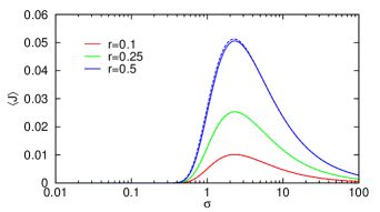
Figure S1: The simplified Eq. 3 in the main text (full line) and the exact result Eq. S19 (dashed) for $\kappa\to\infty$. For small $r\lesssim 0.25$ the results are indistinguishable.

Importantly, Eq. S19 can also be derived by calculating the equilibrium occupancy of the potentials according to the Boltzmann distribution. We define the probability weight in the $\delta a<1$ region as

$$W^{\delta a<1}=\int_{-\infty}^{1}\delta a\ e^{-\beta V_{\rm eff}(\delta a)}$$ (S20)

with $\beta=2/\sigma^{2}$, and similarly for $W_{\pm}^{\delta a>1}$. By comparison to Eq. S13, it can then readily be seen that $W^{\delta a<1}\sim T^{\delta a<1}/\varepsilon$, and the net drift follows straightforwardly.

References

- (1) H.C. Berg and D.A. Brown. Nature, 239:500–504, 1972.
- (2) H.C. Berg. E. coli in Motion. Springer-Verlag, New York, 2004.
- (3) J.E. Segall, S.M. Block, and H.C. Berg. Proc. Natl Acad. Sci. USA, 83:8987–8991, 1986.
- (4) V. Sourjik and H.C. Berg. Proc. Natl Acad. Sci. USA, 99:123–127, 2002.
- (5) E. Korobkova, T. Emonet, J.M.G. Vilar, T.S. Shimizu, and P. Cluzel. Nature, 428:574–578, 2004.
- (6) T.S. Shimizu, Y. Tu, and H.C. Berg. Mol. Syst. Biol., 6:382, 2010.
- (7) Y. Tu and G. Grinstein. Phys. Rev. Lett., 94:208101, 2005.
- (8) F. Matthäus, M. Jagodič, and J. Dobnikar. Biophys. J., 97:946–957, 2009.
- (9) T. Emonet and P. Cluzel. Proc. Natl Acad. Sci. USA, 105:3304–3309, 2008. M.W. Sneddon, W. Pontius, and T. Emonet. Proc. Natl Acad. Sci. USA, 109:805–810, 2012.
- (10) L. Jiang, Q. Ouyang, and Y. Tu. PLoS Comput. Biol., 6:e1000735, 2010.
- (11) Y. Tu, T.S. Shimizu, and H.C. Berg. Proc. Natl Acad. Sci. USA, 105:14855–14860, 2008.
- (12) D. Bray, M.D. Levin, and K. Lipkow. Curr. Biol., 17:12–19, 2007.
- (13) D.A. Clark and L.C. Grant. Proc. Natl Acad. Sci. USA, 102:9150–9155, 2005.
- (14) A. Celani and M. Vergassola. Proc. Natl Acad. Sci. USA, 107:1391–1396, 2010.
- (15) P. Cluzel, M. Surette, and S. Leibler. Science, 287:1652–1655, 2000.
- (16) R. Erban and H.G. Othmer. SIAM J. Appl. Math., 65:361–391, 2004.
- (17) P. Reimann. Phys. Rep., 361:57–265, 2002.
- (18) L. Gammaitoni, P. Hänggi, H. Jung, and F. Marchesoni. Rev. Mod. Phys., 70:223–287, 1998.
- (19) U. Alon, L. Camarena, M.G. Suretter, B.A. Arcas, and Y. and Liu. EMBO J., 17:4238–4248, 1998.
- (20) C.W. Gardiner. Handbook of Stochastic Methods for Physics, Chemistry and the Natural Sciences, 2nd edition. Springer-Verlag, Berlin, 1985.