Conditional simulation of max-stable processes

Abstract

Since many environmental processes such as heat waves or precipitation are spatial in extent, it is likely that a single extreme event affects several locations and the areal modelling of extremes is therefore essential if the spatial dependence of extremes has to be appropriately taken into account. This paper proposes a framework for conditional simulations of max-stable processes and give closed forms for Brown–Resnick and Schlather processes. We test the method on simulated data and give an application to extreme rainfall around Zurich and extreme temperature in Switzerland. Results show that the proposed framework provides accurate conditional simulations and can handle real-sized problems.

1 Introduction

Max-stable processes arise naturally when studying extremes of stochastic processes and therefore play a major role in the statistical modelling of spatial extremes (Buishand et al, 2008; Padoan et al., 2010; Davison et al., 2011). Although a different spectral characterization of max-stable processes exists (de Haan, 1984), for our purposes the most useful representation is (Schlather, 2002)

$$Z(x)=\max_{i\geq 1}\zeta_{i}Y_{i}(x),\qquad x\in\mathbb{R}^{d},$$ (1)

where $\{\zeta_{i}\}_{i\geq 1}$ are the points of a Poisson process on $(0,\infty)$ with intensity $\mbox{d$\Lambda$}(\zeta)=\zeta^{-2}\mbox{d$\zeta$}$ and $Y_{i}$ are independent replicates of a non-negative continuous sample path stochastic process $Y$ such that ${\rm\it E}\{Y(x)\}=1$ for all $x\in\mathbb{R}^{d}$. It is well known that $Z$ is a max-stable process on $\mathbb{R}^{d}$ with unit Fréchet margins (de Haan & Fereira, 2006; Schlather, 2002). Although (1) takes the pointwise maximum over an infinite number of points $\{\zeta_{i}\}$ and processes $Y_{i}$, it is possible to get approximate realizations from $Z$ (Schlather, 2002; Oesting et al., 2011).

Based on (1) several parametric max-stable models have been proposed (Schlather, 2002; Brown & Resnick, 1977; Kabluchko et al., 2009; Davison et al., 2011) and share the same finite dimensional distribution functions

$${\rm pr}\{Z(x_{1})\leq z_{1},\ldots,Z(x_{k})\leq z_{k}\}=\exp\left[-{\rm\it E}\left\{\max_{j=1,\ldots,k}\frac{Y(x_{j})}{z_{j}}\right\}\right],$$

where $k\in\mathbb{N}$, $z_{1},\ldots,z_{k}>0$ and $x_{1},\ldots,x_{k}\in\mathbb{R}^{d}$.

Apart from the Smith model (Genton et al., 2011), only the bivariate cumulative distribution functions are explicitly known. To bypass this hurdle, de Haan & Pereira (2006) propose a semi-parametric estimator and Padoan et al. (2010) suggest the use of the maximum pairwise likelihood estimator.

Paralleling the use of the variogram in classical geostatistics, the extremal coefficient function (Schlather & Tawn, 2003; Cooley et al., 2006)

$$\theta(x_{1}-x_{2})=-z\log{\rm pr}\{Z(x_{1})\leq z,Z(x_{2})\leq z\}$$

is widely used to summarize the spatial dependence of extremes. It takes values in the interval $[1,2]$; the lower bound indicates complete dependence, and the upper one independence.

The last decade has seen many advances to develop a geostatistic of extremes and software is available to practitioners (Wang, 2010; Schlather, 2011; Ribatet, 2011). However an important tool currently missing is conditional simulation of max-stable processes. In classical geostatistic based on Gaussian models, conditional simulations are well established (Chilès & Delfiner, 1999) and provide a framework to assess the distribution of a Gaussian random field given values observed at fixed locations. For example, conditional simulations of Gaussian processes have been used to model land topography (Mandelbrot, 1982).

Conditional simulation of max-stable processes is a long-standing problem (Davis & Resnick, 1989, 1993). Wang & Stoev (2011) provide a first solution, but their framework is limited to processes having a discrete spectral measure and thus may be too restrictive to appropriately model the spatial dependence in complex situations.

Based on the recent developments on the regular conditional distribution of max-infinitely divisible processes, the aim of this paper is to provide a methodology to get conditional simulations of max-stable processes with continuous spectral measures. More formally for a study region $\mathcal{X}\subset\mathbb{R}^{d}$, our goal is to derive an algorithm to sample from the regular conditional distribution of $Z\mid\{Z(x_{1})=z_{1},\ldots,Z(x_{k})=z_{k}\}$ for some $z_{1},\ldots,z_{k}>0$ and $k$ conditioning locations $x_{1},\ldots,x_{k}\in\mathcal{X}$.

2 Conditional simulation of max-stable processes

2.1 General framework

This section reviews some key results of an unpublished paper available from the first author with a particular emphasis on max-stable processes. Our goal is to give a more practical interpretation of their results from a simulation perspective. To this aim, we recall two key results and propose a procedure to get conditional realizations of max-stable processes.

Let $\mathbb{R}^{\mathcal{X}}$ be the space of on $\mathcal{X}\subset\mathbb{R}^{d}$ and let $\Phi=\{\varphi_{i}\}_{i\geq 1}$ be a Poisson point process on $\mathbb{R}^{\mathcal{X}}$ where $\varphi_{i}(x)=\zeta_{i}Y_{i}(x)$ $(i=1,2,\ldots)$ with $\zeta_{i}$ and $Y_{i}$ as in (1). We write $f({x})=\{f(x_{1}),\ldots,f(x_{k})\}$ for all random functions $f\colon\mathcal{X}\to\mathbb{R}$ and ${x}=(x_{1},\ldots,x_{k})\in\mathcal{X}^{k}$. It is not difficult to show that for all Borel set $A\subset\mathbb{R}^{k}$, the Poisson point process $\{\varphi_{i}({x})\}_{i\geq 1}$ defined on $\mathbb{R}^{k}$ has intensity measure

$$\Lambda_{x}(A)=\int_{0}^{\infty}{\rm pr}\left\{\zeta Y(x)\in A\right\}\zeta^{-2}\mbox{d$\zeta$}.$$

The point process $\Phi$ is called regular if the intensity measure $\Lambda_{x}$ has an intensity function $\lambda_{x}$, i.e., $\Lambda_{x}(\mbox{d$z$})=\lambda_{x}(z)\mbox{d$z$}$, for all $x\in\mathcal{X}^{k}$.

The first key point is that provided the point process $\Phi$ is regular, the intensity function $\lambda_{x}$ and the conditional intensity function

$$\lambda_{s\mid x,z}(u)=\frac{\lambda_{(s,x)}(u,z)}{\lambda_{x}(z)},\qquad(s,x)\in\mathcal{X}^{m+k},\qquad u\in\mathbb{R}^{m},\qquad z\in(0,+\infty)^{k},$$ (2)

drives how the conditioning terms $\{Z(x_{j})=z_{j}\}$ $(j=1,\ldots,k)$ are met.

The second key point is that, conditionally on $Z(x)=z$, the Poisson point process $\Phi$ can be decomposed into two independent point processes, say $\Phi=\Phi^{-}\cup\Phi^{+}$, where

$$\Phi^{-} =\{\varphi\in\Phi\colon\text{$\varphi(x_{i})<z_{i}$ for all $i=1,\ldots,k$}\},$$

$$\Phi^{+} =\{\varphi\in\Phi\colon\text{$\varphi(x_{i})=z_{i}$ for some $i=1,\ldots,k$}\}.$$

Before introducing a procedure to get conditional realizations of max-stable processes, we introduce notation and make connections with the pioneering work of Wang & Stoev (2011).

A function $\varphi\in\Phi^{+}$ such that $\varphi(x_{i})=z_{i}$ for some $i\in\{1,\ldots,k\}$ is called an extremal function associated to $x_{i}$ and denoted by $\varphi_{x_{i}}^{+}$. It is easy to show that there exists almost surely a unique extremal function associated to $x_{i}$. Although $\Phi^{+}=\{\varphi_{x_{1}}^{+},\ldots,\varphi_{x_{k}}^{+}\}$ almost surely, it might happen that a single extremal function contributes to the random vector $Z({x})$ at several locations $x_{i}$, e.g., $\varphi^{+}_{x_{1}}=\varphi^{+}_{x_{2}}$. To take such repetitions into account, we define a random partition $\theta=(\theta_{1},\ldots,\theta_{\ell})$ of the set $\{x_{1},\ldots,x_{k}\}$ into $\ell=|\theta|$ blocks and extremal functions $(\varphi_{1}^{+},\ldots,\varphi_{\ell}^{+})$ such that $\Phi^{+}=\{\varphi_{1}^{+},\ldots,\varphi_{\ell}^{+}\}$ and $\varphi_{j}^{+}(x_{i})=z_{i}$ if $x_{i}\in\theta_{j}$ and $\varphi_{j}^{+}(x_{i})<z_{i}$ if $x_{i}\notin\theta_{j}$ $(i=1,\ldots,k;\ j=1,\ldots,\ell)$. Wang & Stoev (2011) call the partition $\theta$ the hitting scenario. The set of all possible partitions of $\{x_{1},\ldots,x_{k}\}$, denoted $\mathscr{P}_{k}$, identifies all possible hitting scenarios.

From a simulation perspective, the fact that $\Phi^{-}$ and $\Phi^{+}$ are independent given $Z(x)=z$ is especially convenient and suggests a three–step procedure to sample from the conditional distribution of $Z$ given $Z(x)=z$.

Theorem 2.1.

Suppose that the point process $\Phi$ is regular and let $(x,s)\in\mathcal{X}^{k+m}$. For $\tau=(\tau_{1},\ldots,\tau_{\ell})\in\mathscr{P}_{k}$ and $j=1,\ldots,\ell$, define $I_{j}=\{i\colon x_{i}\in\tau_{j}\}$, ${x}_{\tau_{j}}=(x_{i})_{i\in I_{j}}$, ${z}_{\tau_{j}}=(z_{i})_{i\in I_{j}}$, ${x}_{\tau_{j}^{c}}=(x_{i})_{i\notin I_{j}}$ and ${z}_{\tau_{j}^{c}}=(z_{i})_{i\notin I_{j}}$. Consider the three–step procedure:

Step 2.2.

Draw a random partition $\theta\in\mathscr{P}_{k}$ with distribution

$$\pi_{x}({z},\tau)={\rm pr}\left\{\theta=\tau\mid Z({x})={z}\right\}=\frac{1}{C({x},{z})}\prod_{j=1}^{|\tau|}\lambda_{{x}_{\tau_{j}}}({z}_{\tau_{j}})\int_{\{{u}_{j}<{z}_{\tau_{j}^{c}}\}}\lambda_{{x}_{\tau_{j}^{c}}\mid{x}_{\tau_{j}},{z}_{\tau_{j}}}({u}_{j})\mbox{d${u}_{j}$},$$

where the normalization constant is

$$C({x},{z})=\sum_{\tilde{\tau}\in\mathscr{P}_{k}}\prod_{j=1}^{|\tilde{\tau}|}\lambda_{{x}_{\tilde{\tau}_{j}}}({z}_{\theta_{j}})\int_{\{{u}_{j}<{z}_{\tilde{\tau}_{j}^{c}}\}}\lambda_{{x}_{\tilde{\tau}_{j}^{c}}\mid{x}_{\tilde{\tau}_{j}},{z}_{\tilde{\tau}_{j}}}({u}_{j})\mbox{d${u}_{j}$}.$$

Step 2.3.

Given $\tau=(\tau_{1},\ldots,\tau_{\ell})$, draw $\ell$ independent random vectors $\varphi_{1}^{+}({s}),\ldots,\varphi_{\ell}^{+}({s})$ from the distribution

$${\rm pr}\left\{\varphi_{j}^{+}({s})\in\mbox{d${v}$}\mid Z({x})={z},\theta=\tau\right\}=\frac{1}{C_{j}}\left\{\int 1_{\{{u}<{z}_{\tau_{j}^{c}}\}}\lambda_{({s},{x}_{\tau_{j}^{c}})\mid{x}_{\tau_{j}},{z}_{\tau_{j}}}({v},{u})\mbox{d${u}$}\right\}\,\mbox{d${v}$}$$

where $1_{\{\cdot\}}$ is the indicator function and

$$C_{j}=\int 1_{\{{u}<{z}_{\tau_{j}^{c}}\}}\lambda_{({s},{x}_{\tau_{j}^{c}})\mid{x}_{\tau_{j}},{z}_{\tau_{j}}}({v},{u})\mbox{d${u}$d${v}$},$$

and define the random vector $Z^{+}({s})=\max_{j=1,\ldots,\ell}\varphi_{j}^{+}({s})$.

Step 2.4.

Independently draw a Poisson point process $\{\zeta_{i}\}_{i\geq 1}$ on $(0,\infty)$ with intensity $\zeta^{-2}\mbox{d$\zeta$}$ and $\{Y_{i}\}_{i\geq 1}$ independent copies of $Y$, and define the random vector

$$Z^{-}({s})=\max_{i\geq 1}\zeta_{i}Y_{i}(s)1_{\{\zeta_{i}Y_{i}(x)<z\}}.$$

Then the random vector $\tilde{Z}({s})=\max\left\{Z^{+}({s}),Z^{-}({s})\right\}$ follows the conditional distribution of $Z({s})$ given $Z({x})={z}$.

The corresponding conditional cumulative distribution function is

$${\rm pr}\left\{Z({s})\leq{a}\mid Z({x})={z}\right\}=\frac{{\rm pr}\{Z({s})\leq{a},Z({x})\leq{z}\}}{{\rm pr}\{Z({x})\leq{z}\}}\sum_{\tau\in\mathscr{P}_{k}}\pi_{x}({z},\tau)\prod_{j=1}^{|\tau|}F_{\tau,j}({a}),$$ (3)

where

$$F_{\tau,j}({a})={\rm pr}\left\{\varphi_{j}^{+}({s})\leq{a}\mid Z({x})={z},\,\theta=\tau\right\}=\frac{\int_{\{{u}<{z}_{\tau_{j}^{c}},{v}<{a}\}}\lambda_{({s},{x}_{\tau_{j}^{c}})\mid{x}_{\tau_{j}},{z}_{\tau_{j}}}({v},{u})\mbox{d${u}$d${v}$}}{\int_{\{{u}<{z}_{\tau_{j}^{c}}\}}\lambda_{{x}_{\tau_{j}^{c}}|{x}_{\tau_{j}},{z}_{\tau_{j}}}({u})\mbox{d${u}$}}.$$

It is clear from (3) that the conditional random field $Z\mid\{Z(x)=z\}$ is not max-stable.

2.2 Distribution of the extremal functions

In this section we derive closed forms for the intensity function $\lambda_{x}(z)$ and the conditional intensity function $\lambda_{s\mid x,z}(u)$ for two widely used max-stable processes; the Brown–Resnick (Brown & Resnick, 1977; Kabluchko et al., 2009) and the Schlather (Schlather, 2002) processes. Details of the derivations of these closed forms are given in the Appendix.

The Brown–Resnick process corresponds to the case where $Y(x)=\exp\{W(x)-\gamma(x)\}$, $x\in\mathbb{R}^{d}$, in (1) with $W$ a centered Gaussian process with stationary increments, semi variogram $\gamma$ and such that $W(o)=0$ almost surely. For $x\in\mathcal{X}^{k}$ and provided the covariance matrix $\Sigma_{x}$ of the random vector $W(x)$ is positive definite, the intensity function is

$$\lambda_{x}(z) =C_{x}\exp\left(-\frac{1}{2}\log{z}^{T}Q_{x}\log z+L_{x}\log z\right)\prod_{i=1}^{k}z_{i}^{-1},\qquad z\in(0,\infty)^{k},$$

with $1_{k}=(1)_{i=1,\ldots,k}$, $\sigma^{2}_{x}=\{\sigma^{2}(x_{i})\}_{i=1,\ldots,k}$,

$$Q_{x} =\Sigma_{x}^{-1}-\frac{\Sigma_{x}^{-1}1_{k}1_{k}^{T}\Sigma_{x}^{-1}}{1_{k}^{T}\Sigma_{x}^{-1}1_{k}},\qquad L_{x}=\frac{1}{2}\left(\frac{1_{k}^{T}\Sigma_{x}^{-1}\sigma^{2}_{x}-2}{1_{k}^{T}\Sigma_{x}^{-1}1_{k}}1_{k}^{T}-{\sigma^{2}_{x}}^{T}\right)\Sigma_{x}^{-1},$$

$$C_{x} =(2\pi)^{(1-k)/2}|\Sigma_{x}|^{-1/2}(1_{k}^{T}\Sigma_{x}^{-1}1_{k})^{-1/2}\exp\left\{\frac{1}{2}\frac{(1_{k}^{T}\Sigma_{x}^{-1}\sigma^{2}_{x}-1)^{2}}{1_{k}^{T}\Sigma_{x}^{-1}1_{k}}-\frac{1}{2}{\sigma^{2}_{x}}^{T}\Sigma_{x}^{-1}\sigma^{2}_{x}\right\},$$

and for all $(s,x)\in\mathcal{X}^{m+k}$, $(u,z)\in(0,\infty)^{m+k}$ and provided the covariance matrix $\Sigma_{(s,x)}$ is positive definite, the conditional intensity function corresponds to a multivariate log-normal probability density function

$$\lambda_{s\mid x,z}({u})=(2\pi)^{-m/2}|\Sigma_{s\mid x}|^{-1/2}\exp\left\{-\frac{1}{2}(\log u-\mu_{s\mid x,z})^{T}\Sigma_{s\mid x}^{-1}(\log u-\mu_{s\mid x,z})\right\}\prod_{i=1}^{m}u_{i}^{-1},$$

where $\mu_{s\mid x,z}\in\mathbb{R}^{m}$ and $\Sigma_{s\mid x}$ are the mean and covariance matrix of the underlying normal distribution and are given by

$$\Sigma_{s\mid x}^{-1}=J_{m,k}^{T}Q_{(s,x)}J_{m,k},\qquad\mu_{s\mid x,z}=\left\{L_{(s,x)}J_{m,k}-\log z^{T}\tilde{J}_{m,k}^{\,T}Q_{(s,x)}J_{m,k}\right\}\Sigma_{s\mid x},$$

with

$$J_{m,k}=\begin{bmatrix}\mbox{Id}_{m}\\ {0}_{k,m}\end{bmatrix},\qquad\tilde{J}_{m,k}=\begin{bmatrix}0_{m,k}\\ \mbox{Id}_{k}\end{bmatrix},$$

where $\mbox{Id}_{k}$ denotes the $k\times k$ identity matrix and $0_{m,k}$ the $m\times n$ null matrix.

The Schlather process considers the case where $Y(x)=(2\pi)^{1/2}\max\{0,\varepsilon(x)\}$, $x\in\mathbb{R}^{d}$, in (1) with $\varepsilon$ a standard Gaussian process with correlation function $\rho$. The associated point process $\Phi$ is not regular and it is more convenient to consider the equivalent representation where $Y(x)=(2\pi)^{1/2}\varepsilon(x)$, $x\in\mathbb{R}^{d}$. For $x\in\mathcal{X}^{k}$ and provided the covariance matrix $\Sigma_{x}$ of the random vector $\varepsilon(x)$ is positive definite, the intensity function is

$$\lambda_{x}(z)=\pi^{-(k-1)/2}|\Sigma_{x}|^{-1/2}a_{x}(z)^{-(k+1)/2}\Gamma\left(\frac{k+1}{2}\right),\qquad z\in\mathbb{R}^{k},$$

where $a_{x}(z)=z^{T}\Sigma_{x}^{-1}z$.

For $(s,x)\in\mathcal{X}^{m+k}$, $(u,z)\in\mathbb{R}^{m+k}$ and provided that the covariance matrix $\Sigma_{(s,x)}$ is positive definite, the conditional intensity function $\lambda_{s\mid x,z}(u)$ corresponds to the density of a multivariate Student distribution with $k+1$ degrees of freedom, location parameter $\mu=\Sigma_{s:x}\Sigma_{x}^{-1}z$, and scale matrix

$$\tilde{\Sigma}=\frac{a_{x}(z)}{k+1}\left(\Sigma_{s}-\Sigma_{s:x}\Sigma_{x}^{-1}\Sigma_{x:s}\right),\qquad\Sigma_{(s,x)}=\begin{bmatrix}\Sigma_{s}&\Sigma_{s:x}\\ \Sigma_{x:s}&\Sigma_{x}\end{bmatrix}.$$

3 Markov chain Monte Carlo sampler

The previous section introduced a procedure to get realizations from the regular conditional distribution of max-stable processes. This sampling scheme amounts to sample from a discrete distribution whose state space corresponds to all possible partitions of the set of conditioning points, see Theorem 2.1 step 1. Hence, even for a moderate number $k$ of conditioning locations, the state space $\mathscr{P}_{k}$ becomes very large and the distribution $\pi_{x}(z,\cdot)$ cannot be computed. It turns out that a Gibbs sampler is especially convenient.

For $\tau\in\mathscr{P}_{k}$, let $\tau_{-j}$ be the restriction of $\tau$ to the set $\{x_{1},\ldots,x_{k}\}\setminus\{x_{j}\}$. Our goal is to simulate from the conditional distribution

$${\rm pr}(\theta\in\cdot\mid\theta_{-j}=\tau_{-j}),$$ (4)

where $\theta\in\mathscr{P}_{k}$ is a random partition which follows the target distribution $\pi_{x}(z,\cdot)$.

Since the number of possible updates is always less than $k$, a combinatorial explosion is avoided. Indeed for $\tau\in\mathscr{P}_{k}$ of size $\ell$, the number of partitions $\tau^{*}\in\mathscr{P}_{k}$ such that $\tau^{*}_{-j}=\tau_{-j}$ for some $j\in\{1,\ldots,k\}$ is

$$b^{+}=\begin{cases}\ell&\text{if $\{x_{j}\}$ is a partitioning set of $\tau$},\\ \ell+1&\text{if $\{x_{j}\}$ is not a partitioning set of $\tau$},\end{cases}$$

since the point $x_{j}$ may be reallocated to any partitioning set of $\tau_{-j}$ or to a new one.

To illustrate consider the set $\{x_{1},x_{2},x_{3}\}$ and let $\tau=(\{x_{1},x_{2}\},\{x_{3}\})$. Then the possible partitions $\tau^{*}$ such that $\tau^{*}_{-2}=\tau_{-2}$ are $(\{x_{1},x_{2}\},\{x_{3}\})$, $(\{x_{1}\},\{x_{2}\},\{x_{3}\})$, $(\{x_{1}\},\{x_{2},x_{3}\})$, while there exists only two partitions such that $\tau^{*}_{-3}=\tau_{-3}$, i.e., $(\{x_{1},x_{2}\},\{x_{3}\})$, $(\{x_{1},x_{2},x_{3}\})$.

The distribution (4) has nice properties. Since for all $\tau^{*}\in\mathscr{P}_{k}$ such that $\tau^{*}_{-j}=\tau_{-j}$ we have

$${\rm pr}[\theta=\tau^{*}\mid\theta_{-j}=\tau_{-j}]=\frac{\pi_{x}({z},\tau^{*})}{{\displaystyle\sum_{\tilde{\tau}\in\mathscr{P}_{k}}\pi_{x}({z},\tilde{\tau})}1_{\{\tilde{\tau}_{-j}=\tau_{-j}\}}}\propto\frac{\prod_{j=1}^{|\tau^{*}|}w_{\tau^{*}\!,j}}{\prod_{j=1}^{|\tau|}w_{\tau,j}},$$ (5)

where

$$w_{\tau,j}=\lambda_{{x}_{\tau_{j}}}({z}_{\tau_{j}})\int_{\{{u}<{z}_{\tau_{j}^{c}}\}}\lambda_{{x}_{\tau^{c}_{j}}\mid{x}_{\tau_{j}},{z}_{\tau_{j}}}({u})\mbox{d${u}$}.$$

Since many factors cancel out on the right hand side of (5), the Gibbs sampler is especially convenient.

The most computationally demanding part of (5) is the evaluation of the integral

$$\int_{\{{u}<{z}_{\tau_{j}^{c}}\}}\lambda_{{x}_{\tau_{j}^{c}}\mid{x}_{\tau_{j}},{z}_{\tau_{j}}}({u})\mbox{d${u}$}.$$

For the Brown–Resnick and Schlather processes, we follow the lines of Genz (1992) and compute these probabilities using a separation of variables method which provides a transformation of the original integration problem to the unit hyper-cube. Further a quasi Monte Carlo scheme and antithetic variable sampling is used to improve efficiency.

Since it is not obvious how to implement a Gibbs sampler whose target distribution has support $\mathscr{P}_{k}$, the remainder of this section gives practical details. For any fixed locations $x_{1},\ldots,x_{k}\in\mathcal{X}$, we first describe how each partition of $\{x_{1},\ldots,x_{k}\}$ is stored. To illustrate consider the set $\{x_{1},x_{2},x_{3}\}$ and the partition $(\{x_{1},x_{2}\};\{x_{3}\})$. This partition is defined as $(1,1,2)$, indicating that $x_{1}$ and $x_{2}$ belong to the same partitioning set labeled $1$ and $x_{3}$ belongs to the partitioning set $2$. There exist several equivalent notations for this partition: for example one can use $(2,2,1)$ or $(1,1,3)$. Since there is a one-one mapping between $\mathscr{P}_{k}$ and the set

$$\mathscr{P}_{k}^{*}=\left\{(a_{1},\ldots,a_{k})\colon i\in\{2,\ldots,k\},\,1=a_{1}\leq a_{i}\leq\max_{1\leq j<i}a_{j}+1,\,a_{i}\in\mathbb{Z}\right\},$$

we shall restrict our attention to the partitions that live in $\mathscr{P}_{k}^{*}$ and going back to our example we see that $(1,1,2)$ is valid but $(2,2,1)$ and $(1,1,3)$ are not.

For $\tau\in\mathscr{P}_{k}^{*}$ of size $\ell$, let $r_{1}=\sum_{i=1}^{k}1_{\{\tau_{i}=a_{j}\}}$ and $r_{2}=\sum_{i=1}^{k}1_{\{\tau_{i}=b\}}$, i.e., the number of conditioning locations that belong to the partitioning sets $a_{j}$ and $b$ where $b\in\{1,\ldots,b^{+}\}$ with

$$b^{+}=\begin{cases}\ell&(r_{1}=1),\\ \ell+1&(r_{1}\neq 1).\end{cases}$$

Then the conditional probability distribution (5) satisfies

$${\rm pr}(\tau_{j}=b\mid\tau_{i}=a_{i},\,i\neq j)\propto 1 (b=a_{j})$$ , (6)

$${\rm pr}(\tau_{j}=b\mid\tau_{i}=a_{i},\,i\neq j)\propto w_{\tau^{*}\!,b}/(w_{\tau,b}w_{\tau,a_{j}}) (r_{1}=1,r_{2}\neq 0,b\neq a_{j})$$ , (7)

$${\rm pr}(\tau_{j}=b\mid\tau_{i}=a_{i},\,i\neq j)\propto w_{\tau^{*}\!,b}w_{\tau^{*}\!,a_{j}}/(w_{\tau,b}w_{\tau,a_{j}}) (r_{1}\neq 1,r_{2}\neq 0,b\neq a_{j})$$ , (8)

$${\rm pr}(\tau_{j}=b\mid\tau_{i}=a_{i},\,i\neq j)\propto w_{\tau^{*}\!,b}w_{\tau^{*}\!,a_{j}}/w_{\tau,a_{j}} (r_{1}\neq 1,r_{2}=0,b\neq a_{j})$$ , (9)

where $\tau^{*}=(a_{1},\ldots,a_{j-1},b,a_{j+1},\ldots,a_{k})$. Although $\tau^{*}$ may not belong to $\mathscr{P}_{k}^{*}$, it corresponds to a unique partition of $\mathscr{P}_{k}$ and we can use the bijection $\mathscr{P}_{k}\to\mathscr{P}_{k}^{*}$ to recode $\tau^{*}$ into an element of $\mathscr{P}_{k}^{*}$. In (6)–(9) the event $\{r_{1}=1,r_{2}=0,b\neq a_{j}\}$ is missing since $\{r_{1}=1,r_{2}=0\}$ implies that $\tau^{*}=\tau$, where the equality has to be understood in terms of elements of $\mathscr{P}_{k}$, and this case has been already taken into account with (6).

Once these conditional weights have been computed, the Gibbs sampler proceeds by updating each element of $\tau$ successively. We use a random scan implementation of the Gibbs sampler (Liu et al., 1995). More precisely, one iteration of the random scan Gibbs sampler selects an element of $\tau$ at random according to a given distribution, say ${p}=(p_{1},\ldots,p_{k})$, and then updates this element. Throughout this paper we will use the uniform random scan Gibbs sampler for which the selection distribution is assumed to be a discrete uniform distribution, i.e., ${p}=(k^{-1},\ldots,k^{-1})$.

4 Simulation Study

Sample path properties of the max-stable models. For the Brown–Resnick model, the variogram parameters are set to ensure that the extremal coefficient function satisfies $\theta(115)=\text{1$\cdot$7}$ while the correlation function parameters are set to ensure that $\theta(100)=\text{1$\cdot$5}$ for the Schlather model. Brown–Resnick: $\gamma(h)=(h/\lambda)^{\kappa}$ Schlather: $\rho(h)=\exp\{-(h/\lambda)^{\kappa}\}$ $\gamma_{1}$: Very wiggly $\gamma_{2}$: Wiggly $\gamma_{3}$: Smooth $\rho_{1}$: Very wiggly $\rho_{2}$: Wiggly $\rho_{3}$: Smooth $\lambda$ 25 54 69 208 144 128 $\kappa$ 0$\cdot$5 1$\cdot$0 1$\cdot$5 0$\cdot$5 1$\cdot$0 1$\cdot$5

In this section we check if our algorithm is able to produce realistic conditional simulations of Brown–Resnick and Schlather processes. For each model, we consider three different sample path properties, as summarized in Table 4. These configurations were chosen such that the spatial dependence structures are similar to our applications in Section 5.

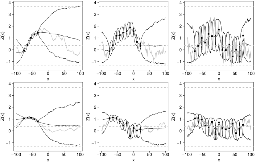
Figure 1: Pointwise sample quantiles estimated from 1000 conditional simulations of max-stable processes with standard Gumbel margins with $k=5,10,15$ conditioning locations. The top row shows results for the Brown–Resnick models with semi variograms $\gamma_{3},\gamma_{2},\gamma_{1}$, from left to right. The bottom row shows results for the Schlather models with correlation functions $\rho_{3},\rho_{2},\rho_{1}$, from left to right. The solid black lines shows the pointwise 0$\cdot$025, 0$\cdot$5, 0$\cdot$975 sample quantiles and the dashed grey lines that of a standard Gumbel distribution. The squares show the conditional points $\{(x_{i},z_{i})\}_{i=1,\ldots,k}$. The solid grey lines correspond the simulated paths used to get the conditioning events.

In order to check if our sampling procedure is accurate and given a single conditional event $\{Z(x)=z\}$ for each configuration, we generated $1000$ conditional realizations with standard Gumbel margins. Figure 1 shows the pointwise sample quantiles obtained from these 1000 simulated paths and compares them to unit Gumbel quantiles. As expected the conditional sample paths inherit the regularity driven by the shape parameter $\kappa$ and there is less variability in regions close to conditioning locations. Since the considered Brown–Resnick processes are ergodic (Kabluchko and Schlather,, 2010), for regions far away from any conditioning location the sample quantiles converges to that of a standard Gumbel distribution indicating that the conditional event has no influence. This is not the case for the non-ergodic Schlather processes. Most of the time the sample paths used to get the conditional events belong to the 95% pointwise confidence intervals, corroborating that our sampling procedure seems to be accurate.

Computational timings for conditional simulations of max-stable processes on a $50\times 50$ grid defined on the square $[0,100\times 2^{1/2}]^{2}$ for a varying number $k$ of conditioning locations uniformly distributed over the region. The timings, in seconds, are mean values over 100 conditional simulations; standard deviations are reported in brackets. Brown–Resnick: $\gamma(h)=(h/25)^{0\cdot 5}$ Schlather: $\rho(h)=\exp\left\{-(h/208)^{0\cdot 50}\right\}$ Step 1 Step 2 Step 3 Overall Step 1 Step 2 Step 3 Overall $k=5$ 0$\cdot$21 (0$\cdot$01) 49 (11) 1$\cdot$4 (0$\cdot$1) 50 (11) 1$\cdot$40 (0$\cdot$02) 1$\cdot$9 (0$\cdot$7) 0$\cdot$9 (0$\cdot$3) 4$\cdot$2 (0$\cdot$8) $k=10$ 8 (2) 76 (18) 1$\cdot$4 (0$\cdot$1) 85 (19) 12 (4) 2$\cdot$4 (0$\cdot$8) 1$\cdot$0 (0$\cdot$3) 15 (4) $k=25$ 95 (38) 117 (30) 1$\cdot$4 (0$\cdot$1) 214 (61) 86 (42) 4 (1) 1$\cdot$0 (0$\cdot$3) 90 (43) $k=50$ 583 (313) 348 (391) 1$\cdot$5 (0$\cdot$1) 931 (535) 367 (222) 62 (113) 1$\cdot$0 (0$\cdot$3) 430 (262) Conditional simulations with $k=5$ do not use a Gibbs sampler.

Table 4 gives computational timings for conditional simulations of max-stable processes on a $50\times 50$ grid with a varying number of conditioning locations. Due to the combinatorial complexity of the partition set $\mathscr{P}_{k}$, the timings increase rapidly with respect to the number of conditioning points $k$. It is however reassuring that the algorithm is tractable when $k\in\{1,\ldots,50\}$; hence covering many practical situations and applications.

5 Application

5.1 Extreme precipitations around Zurich

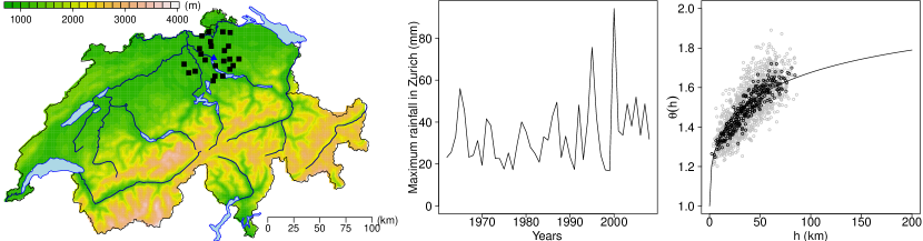
Figure 2: Left: Map of Switzerland showing the stations of the 24 rainfall gauges used for the analysis, with an insert showing the altitude. The station marked with a triangle corresponds to Zurich. Middle: Summer maximum rainfall values for 1962–2008 at Zurich. Right: Comparison between the pairwise extremal coefficient estimates for the 51 original weather stations and the extremal coefficient function derived from a fitted Brown–Resnick processes having semi variogram $\gamma(h)=(h/\lambda)^{\kappa}$. The grey points are pairwise estimates; the black ones are binned estimates and the curve is the fitted extremal coefficient function.

In this section we obtain conditional simulations of extreme precipitation fields. The data considered here were previously analyzed by Davison et al. (2011) who showed that Brown–Resnick processes were one of the most competitive models among various statistical models for spatial extremes.

The data are summer maximum rainfall for the years 1962–2008 at 51 weather stations in the Plateau region of Switzerland, provided by the national meteorological service, MeteoSuisse. To ensure strong dependence between the conditioning locations, we consider as conditional locations the 24 weather stations that are at most 30km apart from Zurich and set as the conditional values the rainfall amounts recorded in the year 2000, the year of the largest precipitation event ever recorded in Zurich between 1962–2008, see Figure 2. The largest and smallest distances between the conditioning locations are around 55km and just over 4km respectively.

A Brown–Resnick process having semi variogram $\gamma(h)=(h/\lambda)^{\kappa}$ has to be fitted and the maximum pairwise likelihood estimator introduced by Padoan et al. (2010) was used to simultaneously fit the marginal parameters and the spatial dependence parameters $\lambda$ and $\kappa$. In accordance with Davison et al. (2011), the marginal parameters were described by $\eta(x)=\beta_{0,\eta}+\beta_{1,\eta}{\rm lon}(x)+\beta_{2,\eta}{\rm lat}(x)$, $\sigma(x)=\beta_{0,\sigma}+\beta_{1,\sigma}{\rm lon}(x)+\beta_{2,\sigma}{\rm lat}(x)$, $\xi(x)=\beta_{0,\xi}$, where $\eta(x),\sigma(x),\xi(x)$ are the location, scale and shape parameters of the generalized extreme value distribution and ${\rm lon}(x),{\rm lat}(x)$ the longitude and latitude of the stations at which the data are observed. The maximum pairwise likelihood estimates for $\lambda$ and $\kappa$ are 38 (14) and 0$\cdot$69 (0$\cdot$07) and give a practical extremal range, i.e., the distance $h_{+}$ such that $\theta(h_{+})=\text{1$\cdot$7}$, of around 115km, see the right panel of Figure 2.

Distribution of the partition size for the rainfall data estimated from a simulated Markov chain of length 15000 Partition size 1 2 3 4 5 6 7–24 Empirical probabilities (%) 66$\cdot$2 28$\cdot$0 4$\cdot$8 0$\cdot$5 0$\cdot$2 0$\cdot$2 $<$0$\cdot$05

Table 5.1 shows the distribution of the partition size estimated from a Markov chain of length 15000. Around 65% of the time the summer maxima observed at the 24 conditioning locations were a consequence of a single extremal function, i.e., only one storm event, and around 30% of the time a consequence of two different storms. Since the simulated Markov chain keeps a trace of all the simulated partitions, we looked at the partitions of size two and saw that around 65% of the time, at least one of the four up–north conditioning locations was impacted by one extremal function while the remaining 20 locations were always influenced by another one.

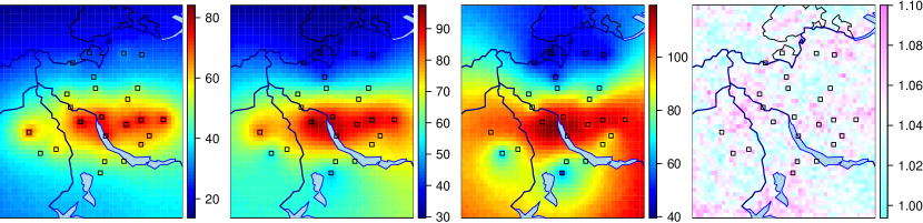
Figure 3: From left to right, maps on a $50\times 50$ grid of the pointwise 0$\cdot$025, 0$\cdot$5 and 0$\cdot$975 sample quantiles for rainfall (mm) obtained from $10000$ conditional simulations of Brown–Resnick processes having semi variogram $\gamma(h)=(h/38)^{\text{0$\cdot$69}}$. The right most panel plots the ratio of the pointwise confidence intervals with and without taking into account the parameter estimate uncertainties. The squares show the conditional locations.

Figure 3 plots the pointwise 0$\cdot$025, 0$\cdot$5 and 0$\cdot$975 sample quantiles obtained from $10000$ conditional simulations of our fitted Brown–Resnick process. The conditional median provides a point estimate for the rainfall at an ungauged location and the 0$\cdot$025 and 0$\cdot$975 conditional quantiles a 95% pointwise confidence interval. As indicated by our simulation study, see Figure 1, the shape parameter $\kappa$ has a major impact on the regularity of paths and on the width of the confidence interval. The value $\hat{\kappa}\approx\text{0$\cdot$69}$ corresponds to very wiggly sample paths and wider confidence intervals. To assess the impact of parameter uncertainties on conditional simulations, the ratio of the width of the confidence intervals with or without parameter uncertainty is shown in the right panel of Figure 3. The uncertainties were taken into account by sampling from the asymptotic distribution of the maximum composite likelihood estimator and draw one conditional simulation for each realization. These ratios show no clear spatial pattern and the width of the confidence interval is increased by an amount of at most 10%.

5.2 Extreme temperatures in Switzerland

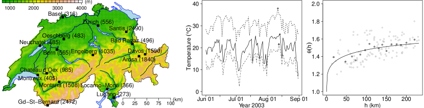
Figure 4: Left: Topographical map of Switzerland showing the sites and altitudes in metres above sea level of 16 weather stations for which annual maxima temperature data are available. Middle: Times series of the daily maxima temperatures at the 16 weather stations for year 2003. The ’$\rm o$’, ’$+$’ and ’$\rm x$’ symbols indicate the annual maxima that occurred the 11th, 12th and 13th of August respectively. Right: Comparison between the fitted extremal coefficient function from a Schlather process (solid red line) and the pairwise extremal coefficient estimates (gray circles). The black circles denote binned estimates with 16 bins.

In this section we apply our results to get conditional simulations of extreme temperature fields. The data considered here were previously analyzed by Davison and Gholam-Rezaee, (2011) and consist in annual maximum temperatures recorded at 16 sites in Switzerland during the period 1961–2005, see Figure 4.

Following the work of Davison and Gholam-Rezaee, (2011), we fit a Schlather process with an isotropic powered exponential correlation function and trend surfaces $\eta(x)=\beta_{0,\eta}+\beta_{1,\eta}{\rm alt}(x)$, $\sigma(x)=\beta_{0,\sigma}$, $\xi(x)=\beta_{0,\xi}+\beta_{1,\xi}{\rm alt}(x)$, where ${\rm alt}(x)$ denotes the altitude above mean sea level in kilometres and $\{\eta(x),\sigma(x),\xi(x)\}$ are the location, scale and shape parameters of the generalized extreme value distribution at location $x$. The spatial dependence parameter estimates are $\hat{\lambda}=260~{}(149)$ and $\hat{\kappa}=0.52~{}(0.12)$ and the corresponding fitted extremal coefficient function, similar to some extent to our test case $\rho_{3}$ in Section 4, is shown in the right panel of Figure 4.

Distribution of the partition size for the temperature data estimated from a Markov chain of length 10000 Partition size 1 2 3 4 5–16 Empirical probabilities (%) 2$\cdot$47 21$\cdot$55 64$\cdot$63 10$\cdot$74 0$\cdot$61

In year 2003, western Europe was hit by a severe heat wave believed to be the hottest one ever recorded since at most 1540 (“2003 European heat wave”, Wikipedia: The Free Encyclopedia). Switzerland was largely impacted by this severe extreme event since the nation wide record temperature of 41$\cdot$5${}^{\circ}{\rm C}$ was recorded that year in Grono, Graubunden, near Lugano. Consequently for our analysis we use as conditional event the maxima temperatures observed in summer 2003, see Figure 4. Based on the fitted Schlather model, we simulate a Markov chain of effective length 10000with a burn-in period of length 500 and a thinning lag of 100 iterations. The distribution of the partition size estimated from these Markov chains is shown in Table 5.2. We can see that around 90% of the time the conditional realizations were a consequence of at most three extremal functions. Since our original observations were not summer maxima but maximum daily values, a close inspection of the times series in year 2003 reveals that the hottest temperatures occurred between the 11th and 13th of August, see Figure 4, and, to some extent, corroborates the distribution of Table 5.2.

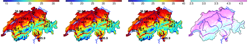
Figure 5: From left to right: Maps on a $64\times 64$ grid of the pointwise 0$\cdot$025, 0$\cdot$5 and 0$\cdot$975 sample quantiles for temperature $(^{\circ}{\rm C})$ obtained from 10000 conditional simulations of the fitted Schlather process. The squares show the conditional locations and the associated conditional values. The right most panel shows temperature anomalies, i.e., the difference between the pointwise conditional and unconditional medians.

Figure 5 shows the 0$\cdot$025, 0$\cdot$5 and 0$\cdot$975 pointwise sample quantiles obtained from 10000 conditional simulations on a $64\times 64$ grid. As expected, we can see that the largest temperatures occurred in the plateau region of Switzerland while temperatures were appreciably cooler in the Alps. The right panel of Figure 5 shows the difference between the pointwise conditional medians and the pointwise unconditional medians estimated from the fitted trend surfaces. The differences range between 2$\cdot$5${}^{\circ}{\rm C}$ and 4$\cdot$75${}^{\circ}{\rm C}$ and the largest deviations occur in the plateau region of Switzerland.

Appendix

The Brown–Resnick model

For all $x\in\mathcal{X}^{k}$ and Borel set $A\subset\mathbb{R}^{k}$

$$\Lambda_{x}(A)=\int_{0}^{\infty}{\rm pr}\left[\zeta\exp\{W(x)-\gamma(x)\}\in A\right]\zeta^{-2}\mbox{d$\zeta$}=\int_{0}^{\infty}\int_{\mathbb{R}^{k}}1_{\{\zeta\exp\{y-\gamma(x)\}\in A\}}f_{x}(y)\mbox{d$y$}\zeta^{-2}\mbox{d$\zeta$},$$

where $f_{x}$ denotes the density of the random vector $W(x)$, i.e., a centered Gaussian random vector with covariance matrix $\Sigma_{x}$ and variance $2\gamma(x)$. The change of variables $z=\zeta\exp\{y-\gamma(x)\}$ and $r=\log\zeta$ yields

$$\Lambda_{x}(A)=\int_{-\infty}^{\infty}\int_{A}f_{x}\{\log z-r+\gamma(x)\}\prod_{i=1}^{k}z_{i}^{-1}\mbox{d$z$}e^{-r}\mbox{d$r$}=\int_{A}\lambda_{x}(z)\mbox{d$z$}$$

with

$$\lambda_{x}(z)=\prod_{i=1}^{k}z_{i}^{-1}\int_{-\infty}^{\infty}f_{x}\{\log z-r+\gamma(x)\}e^{-r}\mbox{d$r$}.$$

Since

$$f_{x}\{\log z-r+\gamma(x)\}e^{-r}=(2\pi)^{-k/2}|\Sigma_{x}|^{-1/2}\exp\left\{-\frac{1}{2}P(r)\right\},$$

with

$$P(r)=r^{2}1_{k}^{T}\Sigma_{x}^{-1}1_{k}-2r\left[1_{k}^{T}\Sigma_{x}^{-1}\{\log z+\gamma(x)\}-1\right]+\{\log z+\gamma(x)\}^{T}\Sigma_{x}^{-1}\{\log z+\gamma(x)\},$$

standard computations for Gaussian integrals give

$$\lambda_{x}(z)=C_{x}\exp\left(-\frac{1}{2}\log{z}^{T}Q_{x}\log z+L_{x}\log z\right)\prod_{i=1}^{k}z_{i}^{-1}.$$

The conditional intensity function is

$$\lambda_{s\mid x,z}(u)=\frac{C_{(s,x)}}{C_{x}}\exp\left\{-\frac{1}{2}\log{(u,z)}^{T}Q_{(s,x)}\log(u,z)+L_{(s,x)}\log(u,z)+\frac{1}{2}\log{z}^{T}Q_{x}\log z-L_{x}\log z\right\}\prod_{i=1}^{m}u_{i}^{-1},$$

and since $\log(u,z)=J_{m,k}\log u+\tilde{J}_{m,k}\log z$, it is not difficult to show that

$$\lambda_{s\mid x,z}({u})=\frac{C_{(s,x)}}{C_{x}}\exp\left\{-\frac{1}{2}(\log u-\mu_{s\mid x,z})^{T}\Sigma_{s\mid x}^{-1}(\log u-\mu_{s\mid x,z})\right\}\prod_{i=1}^{m}u_{i}^{-1}.$$

Finally, the relation $C_{(s,x)}/C_{x}=(2\pi)^{-m/2}|\Sigma_{s\mid x}|^{-1/2}$ is a simple consequence of the normalization $\int\lambda_{s\mid x,z}({u})\mbox{d$u$}=1$.

The Schlather model

For all $x\in\mathcal{X}^{k}$ and Borel set $A\subset\mathbb{R}^{k}$

$$\Lambda_{x}(A)=\int_{0}^{\infty}{\rm pr}[\sqrt{2\pi}\zeta\varepsilon(x)\in A]\zeta^{-2}\mbox{d$\zeta$}=\int_{0}^{\infty}\int_{\mathbb{R}^{k}}1_{\left\{\sqrt{2\pi}\zeta y\in A\right\}}f_{\mathbf{x}}(y)\mbox{d$y$}\zeta^{-2}\mbox{d$\zeta$},$$

where $f_{x}$ denotes the density of the random vector $\varepsilon(x)$, i.e., a centered Gaussian random vector with covariance matrix $\Sigma_{x}$. The change of variable $z=\sqrt{2\pi}\zeta y$ gives

$$\Lambda_{x}(A) =(2\pi)^{-k/2}\int_{0}^{\infty}\int_{A}f_{x}\left(\frac{z}{\sqrt{2\pi}\zeta}\right)\zeta^{-(k+2)}\mbox{d$z$d$\zeta$}$$

$$=(2\pi)^{-k}|\Sigma_{x}|^{-1/2}\int_{0}^{\infty}\int_{A}\exp\left(-\frac{1}{4\pi\zeta^{2}}z^{T}\Sigma_{x}^{-1}z\right)\zeta^{-(k+2)}\mbox{d$z$d$\zeta$}$$

$$=(2\pi)^{-k}|\Sigma_{x}|^{-1/2}\int_{A}\frac{2\pi}{z^{T}\Sigma_{x}^{-1}z}\mathbb{E}[X^{k-1}]\mbox{d$z$},\qquad X\sim\text{Weibull}\left(\sqrt{\frac{4\pi}{z^{T}\Sigma_{x}^{-1}z}},2\right)$$

$$=(2\pi)^{-k}|\Sigma_{x}|^{-1/2}\int_{A}\frac{2\pi}{z^{T}\Sigma_{x}^{-1}z}\left(\frac{4\pi}{z^{T}\Sigma_{x}^{-1}z}\right)^{(k-1)/2}\Gamma\left(\frac{k+1}{2}\right)\mbox{d$z$}$$

$$=\int_{A}\lambda_{\mathbf{x}}(z)\mbox{d$z$},$$

where $\lambda_{x}(z)=\pi^{-(k-1)/2}|\Sigma_{x}|^{-1/2}a_{x}(z)^{-(k+1)/2}\Gamma\left\{(k+1)/2\right\}$ and $a_{x}(z)=z^{T}\Sigma_{x}^{-1}z$.

For all $u\in\mathbb{R}^{m}$ the conditional intensity function is

$$\lambda_{s\mid x,z}(u)=\pi^{-m/2}\frac{|\Sigma_{(s,x)}|^{-1/2}}{|\Sigma_{x}|^{-1/2}}\left\{\frac{a_{(s,x)}(u,z)}{a_{x}(z)}\right\}^{-(m+k+1)/2}a_{x}(z)^{-m/2}\frac{\Gamma\left(\frac{m+k+1}{2}\right)}{\Gamma\left(\frac{k+1}{2}\right)}.$$

We start by focusing on the ratio $a_{(s,x)}(u,z)/a_{x}(z)$. Since

$$\begin{bmatrix}\Sigma_{s}&\Sigma_{s:x}\\ \Sigma_{x:s}&\Sigma_{x}\end{bmatrix}^{-1}=\begin{bmatrix}(\Sigma_{s}-\Sigma_{s:x}\Sigma_{x}^{-1}\Sigma_{x:s})^{-1}&-(\Sigma_{s}-\Sigma_{s:x}\Sigma_{x}^{-1}\Sigma_{x:s})^{-1}\Sigma_{s:x}\Sigma_{x}^{-1}\\ -\Sigma_{x}^{-1}\Sigma_{x:s}(\Sigma_{s}-\Sigma_{s:x}\Sigma_{x}^{-1}\Sigma_{x:s})^{-1}&\Sigma_{x}^{-1}+\Sigma_{x}^{-1}\Sigma_{x:s}(\Sigma_{s}-\Sigma_{s:x}\Sigma_{x}^{-1}\Sigma_{x:s})^{-1}\Sigma_{s:x}\Sigma_{x}^{-1}\end{bmatrix},$$

straightforward algebra shows that

$$\frac{a_{(s,x)}(u,z)}{a_{x}(z)}=1+\frac{(u-\mu)^{T}\tilde{\Sigma}^{-1}(u-\mu)}{k+1},\qquad\mu=\Sigma_{s:x}\Sigma_{x}^{-1}z,\qquad\tilde{\Sigma}=\frac{a_{x}(z)}{k+1}\left(\Sigma_{s}-\Sigma_{s:x}\Sigma_{x}^{-1}\Sigma_{x:s}\right).$$

We now try to simplify the ratio $|\Sigma_{(s,x)}|/|\Sigma_{x}|$. Using the fact that

$$\Sigma_{(s,x)}=\begin{bmatrix}\Sigma_{s}&\Sigma_{s:x}\\ \Sigma_{x:s}&\Sigma_{x}\end{bmatrix}=\begin{bmatrix}\mbox{Id}_{m}&\Sigma_{s:x}\\ 0_{k,m}&\Sigma_{x}\end{bmatrix}\begin{bmatrix}\Sigma_{s}-\Sigma_{s:x}\Sigma_{x}^{-1}\Sigma_{x:s}&0_{m,k}\\ \Sigma_{x}^{-1}\Sigma_{x:s}&\mbox{Id}_{k}\end{bmatrix},$$

combined with some more algebra yields

$$\frac{|\Sigma_{(s,x)}|}{|\Sigma_{x}|}=|\Sigma_{s}-\Sigma_{s:x}\Sigma_{x}^{-1}\Sigma_{x:s}|=\left\{\frac{k+1}{a_{x}(z)}\right\}^{m}|\tilde{\Sigma}|.$$

Using the two previous results it is easily found that

$$\lambda_{s\mid x,z}(u)=\pi^{-m/2}(k+1)^{-m/2}|\tilde{\Sigma}|^{-1/2}\left\{1+\frac{(u-\mu)^{T}\tilde{\Sigma}^{-1}(u-\mu)}{k+1}\right\}^{-(m+k+1)/2}\frac{\Gamma\left(\frac{m+k+1}{2}\right)}{\Gamma\left(\frac{k+1}{2}\right)},$$

which corresponds to the density of a multivariate Student distribution with the expected parameters.

References

• Brown & Resnick (1977) Brown, B. M. & Resnick, S. I. (1977). Extreme values of independent stochastic processes. J. Appl. Prob. 14, 732–739.
• Buishand et al (2008) Buishand, T. A., de Haan, L. & Zhou, C. (2008). On spatial extremes: With application to a rainfall problem. Annals of Applied Statistics 2, 624–642.
• Chilès & Delfiner (1999) Chilès, J.-P. & Delfiner, P. (1999). Geostatistics: Modelling Spatial Uncertainty. New York: Wiley.
• Cooley et al. (2006) Cooley, D., Naveau, P. & Poncet, P. (2006). Variograms for spatial max-stable random fields. In Dependence in Probability and Statistics, vol. 187 of Lecture Notes in Statistics. New York: Springer, pp. 373–390.
• Davis & Resnick (1989) Davis, R. & Resnick, S. (1989). Basic properties and prediction of max-arma processes. Advances in Applied Probability 21, 781–803.
• Davis & Resnick (1993) Davis, R. & Resnick, S. (1993). Prediction of stationary max-stable processes. Annals Of Applied Probability 3, 497–525.
• Davison and Gholam-Rezaee, (2011) Davison, A. C. & Gholam-Rezaee, M. M. (2011). Geostatistics of extremes. Proceedings of the Royal Society A: Mathematical, Physical and Engineering Science.
• Davison et al. (2011) Davison, A. C., Padoan, S. A. & Ribatet, M. (2011). Statistical modelling of spatial extremes. To appear in Statistical Science.
• de Haan (1984) de Haan, L. (1984). A spectral representation for max-stable processes. The Annals of Probability 12, 1194–1204.
• de Haan & Pereira (2006) de Haan, L. & Pereira, T. T. (2006). Spatial extremes: Models for the stationary case. The annals of Statistics 34, 146–168.
• de Haan & Fereira (2006) de Haan, L. & Fereira, A. (2006). Extreme value theory: An introduction. Springer Series in Operations Research and Financial Engineering.
• Genton et al. (2011) Genton, M. G., Ma, Y. & Sang, H. (2011). On the likelihood function of Gaussian max-stable processes. Biometrika 98, 481–488.
• Genz (1992) Genz, A. (1992). Numerical computation of multivariate normal probabilities. J. Comp. Graph Stat 1, 141–149.
• Kabluchko et al. (2009) Kabluchko, Z., Schlather, M. & de Haan, L. (2009). Stationary max-stable fields associated to negative definite functions. Ann. Prob. 37, 2042–2065.
• Kabluchko and Schlather, (2010) Kabluchko, Z. & Schlather, M. (2010). Ergodic properties of max-infinitely divisible processes. Stochastic Processes and their Applications, 120(3):281–295.
• Liu et al. (1995) Liu, J., Wong, W. & Kong, A. (1995). Correlation structure and convergence rate of the Gibbs sampler with various scans. Journal of the Royal Statistical Society Series B 57, 157–169.
• Mandelbrot (1982) Mandelbrot, B. (1982). The fractal geometry of nature. W. H. Freeman.
• Oesting et al. (2011) Oesting, M., Kabluchko, Z. & Schlather, M. (2011). Simulation of Brown–Resnick processes. To appear in Extremes.
• Padoan et al. (2010) Padoan, S. A., Ribatet, M. & Sisson, S. (2010). Likelihood-based inference for max-stable processes. Journal of the American Statistical Association 105, 263–277.
• R Development Core Team (2011) R Development Core Team (2011). R: A Language and Environment for Statistical Computing. R Foundation for Statistical Computing, Vienna, Austria. ISBN 3-900051-07-0.
• Ribatet (2011) Ribatet, M. (2011). SpatialExtremes: Modelling Spatial Extremes. R package version 1.8-5.
• Schlather (2002) Schlather, M. (2002). Models for stationary max-stable random fields. Extremes 5, 33–44.
• Schlather (2011) Schlather, M. (2011). RandomFields: Simulation and Analysis of Random Fields. R package version 2.0.53.
• Schlather & Tawn (2003) Schlather, M. & Tawn, J. (2003). A dependence measure for multivariate and spatial extremes: Properties and inference. Biometrika 90, 139–156.
• Wang (2010) Wang, Y. (2010). maxLinear: Conditional samplings for max-linear models. R package version 1.0.
• Wang & Stoev (2011) Wang, Y. & Stoev, S. A. (2011). Conditional sampling for spectrally discrete max-stable random fields. Advances in Applied Probability 43, 461–483.