On unorthodox solutions of the Bloch equations

abstract

A systematic, rigorous, and complete investigation of the Bloch equations in time-harmonic driving classical field is performed. Our treatment is unique in that it takes full advantage of the partial fraction decomposition over real number field, which makes it possible to find and classify all analytic solutions. Torrey’s analytic solution in the form of exponentially damped harmonic oscillations [Phys. Rev. 76, 1059 (1949)] is found to dominate the parameter space, which justifies its use at numerous occasions in magnetic resonance and in quantum optics of atoms, molecules, and quantum dots. The unorthodox solutions of the Bloch equations, which do not have the form of exponentially damped harmonic oscillations, are confined to rather small detunings $\delta^{2}\lesssim(\gamma-\gamma_{t})^{2}/27$ and small field strengths $\Omega^{2}\lesssim 8(\gamma-\gamma_{t})^{2}/27$, where $\gamma$ and $\gamma_{t}$ describe decay rates of the excited state (the total population relaxation rate) and of the coherence, respectively. The unorthodox solutions being readily accessible experimentally are characterized by rather featureless time dependence.

Keywords: analytic solutions * Bloch equations * two-level system * time-harmonic driving field

PACS codes: 03.67.-a, 42.50.-p, 82.56.-b, 33.50.-j

1 Introduction

The Bloch equations in time-harmonic driving classical field have been employed over several decades as an important tool in studies of many different physical phenomena [1, 2, 3, 4, 5, 6, 7, 8, 9, 10, 11, 12, 13, 14, 15, 16]. The equations [see (2) below] underline the theory of magnetic resonance [1, 2, 3, 4, 5] and the quantum optics of a two-level atom (molecule, spin, ion, etc) driven by a classical field [3, 6, 7, 8, 9, 10, 11, 12, 13, 14]. The latter problem is one of the most discussed and is at the heart of the theory of self-induced transparency [6, 8], the susceptibility of an ensemble of atoms (spins, ions, etc) in gain media [9], and a number of other optical phenomena [8, 9, 10, 11, 12, 13]. Recently the problem has been extensively studied in connection with the proposed use of atoms and molecules as a triggered single-photon emitter [11, 13], a single-photon emission of resonantly driven semiconductor quantum dot in a microcavity [15], and decoherence in dc SQUID phase qubits [16]. Advances in the fabrication of single defect centres in diamond enable one to investigate two-level diamond-based single-photon emitters at room temperatures [17, 18]. At the same time the single defect centres enable nanoscale magnetic sensing, and hence a nanoscale imaging magnetometry, with an individual electronic spin in diamond under ambient conditions [19, 20, 21].

The Bloch equations form a linear system of three ordinary differential equations [see (2) below], which can be formally solved in the following three steps:

• (i) applying the Laplace transform, whereby the system of differential equations reduces to a linear algebra problem;

• (ii) solving the ensuing linear algebra problem (for instance, by means of Cramer’s rule);

• (iii) applying the inverse Laplace transform.

That was also the original Torrey’s approach [2, 7, 8], who established a general time dependence of each Bloch variable $u_{l}$, $l=1,\,2,\,3$, in the form of exponentially damped harmonic oscillations

$$u_{l}(t)=A_{0}+A_{1}e^{-\kappa_{1}t}+A_{2}e^{-bt}\cos(st)+(A_{3}/s)e^{-bt}\sin(st).$$ (1)

In order to determine explicit analytic solutions, essential to Torrey’s approach was to find out a negative real root $-\kappa_{1}$ (it always exists - see section 3) of a characteristic determinant $\Delta$ [see (10) below] of the Bloch equations. Assuming the knowledge of $\kappa_{1}$, Torrey [2] determined the constants $A_{0}$, $A_{1}$ as certain limits of Laplace transforms [see (55), (56) below], and determined the remaining constants $A_{2}$, $A_{3}$ using the initial conditions and the knowledge of $A_{0}$ and $A_{1}$ (see Eqs. (45)-(47) of [2]). The root parameters $b$ and $s$ were then determined on comparing expansion coefficients of the cubic polynomial $\Delta(p)$ in the Laplace transform variable $p$ against corresponding expressions of the coefficients in terms of cubic roots [see Eq. (48) of [2] and (16) below]. Not aware of Cardano’s formula [24] - a jewel of the mathematics of the $16$th century [25] - Torrey managed to formulate explicit analytic solutions merely in three special situations [2]:

• strong collisions: $\gamma=\gamma_{t}$ (T1);

• exact resonance: $\delta=0$ (T2);

• intense external field: $\Omega/\gamma_{t}\gg 1$ (T3).

Additionally, it had long remained unnoticed that Torrey’s general solution (1) had been confined to the parameter range when the discriminant $D$ [see (18) below] [27] of the characteristic determinant $\Delta$ is negative (see section 5). Indeed, general solutions in the parameter range $D>0$ are nonoscillating and can be represented as a sum of three exponentially damped terms, wherein each term corresponds to a real cubic root of the characteristic determinant $\Delta$ (see section 5).

Surprisingly enough, the limitation of Torrey’s general solution (1) to the parameter range $D<0$ and the unawareness of Cardano’s formula had been since without exception repeated in the literature [2, 7] and in textbooks (cf section 3.5 of Ref. [8]) for several decades. The latter is quite remarkable given the role that Torrey’s analytic solutions played in quantum optics and magnetic resonance literature [7, 8]. It took several decades before Hore and McLauchlan had finally made use of Cardano’s formula [24] and formally determined the cubic roots [4]. However, their analytic solution has other deficiencies to be discussed in section 8.

In what follows, we closely follow the original Torrey’s approach [2, 4, 5] and supplement it with two additional elementary tools:

• (i) the partial fraction expansion, or partial fraction decomposition (PFD) [23] over the field of real numbers (see Appendix A), combined with the classification of roots of a real cubic polynomial, and

• (ii) a fully compensated formula for real roots of a real cubic polynomial [see (38) below], which has recently been derived [26] from Cardano’s formula [24].

The first tool will enable one to classify and, up to an explicit knowledge of the roots of $\Delta$, determine all the possible functional forms of solutions of the Bloch equations (2) for all values of $D\lesseqqgtr 0$. The second tool will allow one to determine the roots of $\Delta$, and hence solutions of the Bloch equations, explicitly.

The outline of the article is as follows. In section 2 we summarize notation and give some basic definitions. In section 3 a full advantage of the partial fraction decomposition over real number field is made, all possible solution types (e.g. of non Torrey type) are classified [see (17)]. In section 4 the parameter range of unorthodox solutions is determined. In section 5 decay constants corresponding to each solution type are determined by Cardano’s formula. In section 6 sufficient and necessary conditions for doubly and triply degenerate real roots are established in terms of the model parameters. Steady state solutions and remaining numerical constants of different solution types [see (17)] are determined in section 7. In section 8 connection to earlier results and various conditions of the applicability of our results are discussed. We then conclude by section 9. A number of formulae and intermediary steps are relegated to Appendices A and B.

2 Bloch equations

The Bloch equations are a linear system of differential equations with constant coefficients for a Bloch vector with components $(u,v,w)$, also known as the Bloch variables [1, 2, 4, 5, 6, 7, 8, 9],

$$u^{\prime} = -\gamma_{t}u-\delta v,$$

$$v^{\prime} = -\gamma_{t}v+\delta u+\Omega\,w,$$

$$w^{\prime} = -\gamma w-\Omega v+\gamma w_{eq},$$ (2)

where the prime denotes derivative with respect to a parameter $t$ defined in Table 1, and $w_{eq}$ is an equilibrium value of $w$. Occasionally we denote the Bloch variables as $(u,v,w)=(u_{1},u_{2},u_{3})$.

Table 1. The Bloch equations parameters in the case of a two-level system and in the case of magnetic resonance (MR).

	two-level system	MR
$t$	time $\tau$	rescaled time $gH_{1}\tau$
$\gamma$	$1/T_{1}$	$1/(gH_{1}T_{1})$
$\gamma_{t}$	$1/T_{2}$	$1/(gH_{1}T_{2})$
$\omega_{0}$	$(\epsilon_{2}-\epsilon_{1})/\hbar$	Larmor frequency $gH_{0}$
$\delta$	$\omega_{0}-\omega$	$(\omega_{0}-\omega)/(gH_{1})$
$\Omega$	$\frac{|{\mbox{\boldmath$\mu$}}\cdot{\bf E}_{0}|}{\hbar}$	$-1$

The meaning of the parameters depends on the problem solved. In the case of a two-level system with energies $\epsilon_{1}$ and $\epsilon_{2}>\epsilon_{1}$ interacting with time-harmonic perturbing classical field $E(t)=E_{0}\cos\omega t$ with the driving frequency $\omega$ and amplitude $E_{0}$, the Bloch variables $u,\,v,\,w$ are related to the elements of a $2\times 2$ hermitian density matrix $\rho_{ij}=\rho_{ji}^{*}$ [7, 9]

$$u=2\mbox{Re }\rho_{12},~{}~{}~{}v=2\mbox{Im }\rho_{12},~{}~{}~{}w=\rho_{22}-\rho_{11}.$$ (3)

The parameter $\delta$ stands for the driving field detuning from the intrinsic resonance frequency $\omega_{0}$, whereas $\Omega$, which reduces to the Rabi frequency at zero detuning, accounts for the interaction strength - it is entirely determined by the coupling with the driving field (e.g. between the electric field amplitude and the transition dipole moment $\mu$) (see Table 1). Phenomenological constants $\gamma$ and $\gamma_{t}$ describe decay rates of the excited state (the total population relaxation rate) and of the coherence, respectively, where $T_{1}$ is the spontaneous emission lifetime and $T_{2}$ (typically $\geq T_{1}$) is the total dephasing time [8, 9]. According to (3), $w$ is the single atom population difference, also called inversion [8, 9]. The condition $w(0)=-1$, which (together with $u_{0}=v_{0}=0$) is often taken as the initial condition [8, 5, 28], means that the two-level atom is initially in its ground state. The third equation in (2) shows that $v$ is the component effective in coupling to the field to produce energy changes. Thus $v$ determines the absorptive (in-quadrature with the field ${\bf E}$) component and $u$ the dispersive (in-phase) component of the atomic transition dipole moment. Note in passing that $w_{eq}$ is not necessary a thermal equilibrium value, since some pump mechanism may be present that causes $w_{eq}$ at equilibrium to have some fixed value that is different from its thermal equilibrium value [9].

In the theory of magnetic resonance of precessing (nuclear or electronic) spins [1, 2, 4, 5], the time constants $T_{2}$ and $T_{1}$ correspond to the longitudinal and transverse relaxation constants [1, 2, 4, 5] and, in contrast to the optics, $T_{2}$ is always less than or equal to $T_{1}$ [22]. Assuming a constant magnetic field ${\bf H}_{0}$ applied along the $z$-axis and a time-harmonic component $2{\bf H}_{1}\cos\omega t$ applied in the $x$-direction, the components $u,v,w$ in Eqs. (2) are formed by the respective $x$, $y$, $z$ components of a nuclear or electron (macroscopic) magnetization ${\bf M}$, and $w_{eq}$ is related to the static magnetization ${\bf M}_{0}=\chi_{0}{\bf H}_{0}$, where $\chi_{0}$ is the static susceptibility [1, 2]. Eqs. (2) are then valid with the time $\tau$ together with the homogeneous lifetimes $T_{1}$ and $T_{2}$ being rescaled by $gH_{1}$, where $g$ is the absolute value of the gyromagnetic ratio (see Table 1).

Importantly, in any case is the ratio $\Omega/|\gamma-\gamma_{t}|$ proportional to the driving field (either ${\bf E}_{0}$ or ${\bf H}_{1}$) and (see Table 1)

$$\frac{\delta}{|\gamma-\gamma_{t}|}=\frac{\omega_{0}-\omega}{\left|\frac{1}{T_{1}}-\frac{1}{T_{2}}\right|}\cdot$$ (4)

3 Classification of possible solution types

Following Torrey’s approach [2, 4, 5], upon applying the Laplace transform,

$$\tilde{f}(p)=\int_{0}^{\infty}f(t)e^{-pt}dt,$$ (5)

the Bloch equations (2) are transformed into the matrix equation

$$\left(\begin{array}[]{ccc}p+\gamma_{t}&\delta&0\\ -\delta&p+\gamma_{t}&-\Omega\\ 0&\Omega&p+\gamma\\ \end{array}\right)\left(\begin{array}[]{c}\tilde{u}\\ \tilde{v}\\ \tilde{w}\end{array}\right)=\left(\begin{array}[]{c}u_{0}\\ v_{0}\\ W_{0}\end{array}\right),$$ (6)

where tilde denotes the Laplace transform of the Bloch variables,

$$W_{0}=w_{0}+\frac{\gamma w_{eq}}{p},$$ (7)

and $u_{0}$, $v_{0}$, $w_{0}$ are the initial values of the Bloch variables. Cramer’s rule then yields

$$\tilde{u}_{l}=\frac{f_{l}(p)}{\Delta(p)},$$ (8)

where $\tilde{u}_{l}$, $l=1,2,3$, stands for $\tilde{u}$, $\tilde{v}$, and $\tilde{w}$, respectively, and

$$f_{l}(p)=\left\{\begin{array}[]{cc}u_{0}[(p+\gamma_{t})(p+\gamma)+\Omega^{2}]-v_{0}\delta(p+\gamma)-W_{0}\delta\Omega,&l=1\\ u_{0}\delta(p+\gamma)+v_{0}(p+\gamma_{t})(p+\gamma)+W_{0}\Omega\,(p+\gamma_{t}),&l=2\\ -u_{0}\delta\Omega-v_{0}\Omega(p+\gamma_{t})+W_{0}[(p+\gamma_{t})^{2}+\delta^{2}],&l=3\end{array}\right.$$ (9)

The determinant $\Delta(p)$ of the coefficient matrix is a real cubic polynomial

$$\Delta(p)=p^{3}+a_{2}p^{2}+a_{1}p+a_{0},$$ (10)

where

$$a_{2} = \gamma+2\gamma_{t},$$ (11)

$$a_{1} = \gamma_{t}^{2}+2\gamma\gamma_{t}+\delta^{2}+\Omega^{2},$$ (12)

$$a_{0} = \gamma\gamma_{t}^{2}+\gamma\delta^{2}+\gamma_{t}\Omega^{2}.$$ (13)

The multiplication of both the numerator and denominator on the right-hand side of (8) by $p$ changes each $f_{l}(p)$ defined by Eqs. (9) into a cubic polynomial, whereas the ratio on the right-hand side of (8) becomes the ratio of a cubic and quartic polynomials. Given that $\Delta(p)$ is a real cubic polynomial [see (11) to (13) for the coefficients $a_{j}$ in (10)], this suggests the application of the PFD over the field of real numbers [see (67) in Appendix A]. The PFD enables one to express the fractions such as that in (8) as a sum of much simpler fractions, whose inverse Laplace transform may be readily available. To this end note [e.g. by the fundamental theorem of algebra (66)] that as any real cubic polynomial, $\Delta(p)$ can have either (i) one real root and a pair of complex conjugate roots or (ii) three real roots. Given that all the coefficients $a_{j}$ in (10) are positive real numbers, one can prove additionally that:

• $\Delta(p)$ has always at least one negative real root (P1);

• if $\Delta(p)$ has three real roots, they are all negative (P2);

• if not all roots of $\Delta(p)$ are real than there is one real root and two complex conjugate (c.c.) roots (P3);

• if at least two roots of $\Delta(p)$ coincide, they are all negative real roots (P4). It may be that $\Delta(p)$ has a double real root and another distinct single real root; alternatively, all three roots of $\Delta(p)$ coincide yielding a triple real root.

The properties P1 and P2 can be shown to be a straightforward consequence of the intermediate value theorem when applied to a cubic polynomial $\Delta(p)$ with positive real coefficients $a_{j}$. Obviously, a sufficient condition for P1 is $\Delta(0)=a_{0}>0$, whereas a sufficient condition for P2 is

$$\Delta(p)>0\hskip 113.81102pt(p\geq 0).$$ (14)

The property P3 follows from P1 and the fundamental theorem of algebra (66) applied to a real cubic polynomial. Eventually, the property P4 follows upon combining P1 to P3. Note in passing that we disregarded a special case of $a_{0}=0$, which is treated at the end of section 7. To this case belongs also the trivial undamped case $\gamma=\gamma_{t}=0$ (which implies both $a_{0}=0$ and $a_{2}=0$), in which case the Bloch equations (2) describe the precession of a classical gyromagnetic moment in a magnetic field [3, 8].

Given the properties P1 to P4, and on writing negative real roots of $\Delta(p)$ as $x_{j}=-\kappa_{j}$, $j=1,2,3$ ($\kappa_{j}>0$), the application of the PFD [see (67) in Appendix A] enables one to decompose each $f_{l}(p)/\Delta(p)$ as

$$\frac{f(p)}{\Delta(p)}=\frac{pf(p)}{p\Delta(p)}=\left\{\begin{array}[]{ll}\frac{A_{0}}{p}+\frac{A_{1}}{p+\kappa_{1}}+\frac{A_{2}(p+b)+A_{3}}{(p+b)^{2}+s^{2}},&\mbox{(pair of c.c. roots)}\\ \frac{A_{0}}{p}+\frac{A_{1}}{p+\kappa_{1}}+\frac{A_{2}}{p+\kappa_{2}}+\frac{A_{3}}{p+\kappa_{3}},&\mbox{(distinct real roots)}\\ \frac{A_{0}}{p}+\frac{A_{1}}{p+\kappa_{1}}+\frac{A_{2}}{p+\kappa_{2}}+\frac{A_{3}}{(p+\kappa_{2})^{2}},&\mbox{(double real root)}\\ \frac{A_{0}}{p}+\frac{A_{1}}{p+\kappa_{1}}+\frac{A_{2}}{(p+\kappa_{1})^{2}}+\frac{A_{3}}{(p+\kappa_{1})^{3}},&\mbox{ (triple real root)}.\end{array}\right.$$ (15)

Herein and below the index $l$ labeling different Bloch variables will be suppressed unless explicitly required. In the first line of Eqs. (15), corresponding to cubic roots $-\kappa_{1}$, $z$, and $\bar{z}$, we have recast the irreducible quadratic factor $(p-z)(p-\bar{z})$ in Torrey’s form $(p+b)^{2}+s^{2}$. Given that the coefficients $a_{2}$ and $a_{0}$ in Eqs. (11) and (13) can be alternatively expressed in terms of cubic roots $z_{1}$, $z_{2}$, and $z_{3}$ of $\Delta(p)$ as $a_{2}=-(z_{1}+z_{2}+z_{3})$ and $a_{0}=-z_{1}z_{2}z_{3}$, the Torrey constants $b$ and $s$ can be entirely expressed in terms of $\kappa_{1}$, $a_{2}$ and $a_{0}$,

$$b=-\mbox{Re }z=\frac{a_{2}-\kappa_{1}}{2},~{}~{}~{}~{}~{}s=\sqrt{|z|^{2}-b^{2}}=\sqrt{\frac{a_{0}}{\kappa_{1}}-b^{2}}.$$ (16)

On substituting (15) back into (8) one can perform the inverse Laplace transform (see Appendix B). Note in passing that the property P2 additionally guarantees the very existence of the inverse Laplace transform. (Indeed, if one of the real roots were positive, one would face singular integrals.) After the inverse Laplace transform one arrives at the following complete set of the possible functional forms of solutions of the Bloch equations (2),

$$u_{l}(t)=\left\{\begin{array}[]{ll}A_{0}+A_{1}e^{-\kappa_{1}t}+A_{2}e^{-bt}\cos(st)+(A_{3}/s)e^{-bt}\sin(st),&\mbox{(pair of c.c. roots)}\\ A_{0}+A_{1}e^{-\kappa_{1}t}+A_{2}e^{-\kappa_{2}t}+A_{3}e^{-\kappa_{3}t},&\mbox{(distinct real roots)}\\ A_{0}+A_{1}e^{-\kappa_{1}t}+A_{2}e^{-\kappa_{2}t}+A_{3}te^{-\kappa_{2}t},&\mbox{ (double root)}\\ A_{0}+A_{1}e^{-\kappa_{1}t}+A_{2}te^{-\kappa_{1}t}+\frac{1}{2}A_{3}t^{2}e^{-\kappa_{1}t},&\mbox{ (triple root)}.\end{array}\right.$$ (17)

The PFD’s given by Eqs. (15) exhaust all the possible PFD’s of the ratio $f(p)/\Delta(p)$. There is no other decomposition possible. Only the first line in Eqs. (15) and (17) corresponds to the Torrey solution [2], whereas remaining lines yield unorthodox (i.e. non Torrey) solutions. Importantly, the PFD guarantees that the respective sets of numerical constants $A_{0}$, $A_{1}$, $A_{2}$, and $A_{3}$ for different Bloch variables, together with constants $b$ and $s$, are all real numbers.

4 Parameter range of unorthodox solutions

To this end, we have not verified yet if any of the above solution types could be attained within the physical range of parameters in the Bloch equations (2). In order to proceed, one needs to determine the value of the discriminant $D$ of $\Delta(p)$. According to [26]

$$D = a_{1}^{2}a_{2}^{2}-4a_{1}^{3}-4a_{0}a_{2}^{3}-27a_{0}^{2}+18a_{0}a_{1}a_{2}$$ (18)

$$= (\gamma-\gamma_{t})^{2}\Omega^{2}\left(\Omega^{2}+20\delta^{2}\right)-4(\gamma-\gamma_{t})^{2}\delta^{2}\left[(\gamma-\gamma_{t})^{2}+2\delta^{2}\right]$$

$$-4(\delta^{2}+\Omega^{2})^{3}.$$

In terms of the roots, the discriminant of a general polynomial of the $n$th order is given by [27]

$$D=a_{n}^{2n-2}\prod_{i<j}{(z_{i}-z_{j})^{2}},$$ (19)

where $a_{n}$ is the leading coefficient [$a_{n}=a_{3}=1$ in (10)] and $z_{1},\ldots,z_{n}$ are the roots (counting multiplicity) of the polynomial. For a cubic polynomial with real coefficients, the use of the general form of the discriminant [27] together with its real value [see (18)] enables one to relate the nature of roots to the value of $D$ as follows:

• $D<0$: a cubic polynomial has one real root and two complex conjugate roots;

• $D>0$: there are three distinct real roots;

• $D=0$: at least two roots coincide, and they are all real.

To this end one can show that Torrey special solutions labeled by T1 and T3 introduced in section 1 are always described by exponentially damped harmonic oscillations. Indeed, in the particular case of strong collisions (T1), Eq. (18) reduces for $\gamma=\gamma_{t}$ to

$$D=-4(\delta^{2}+\Omega^{2})^{3}<0.$$ (20)

In the particular case of intense external field (T3), Eq. (18) reduces for $\Omega\gg\gamma_{t},\,\gamma$ to

$$D=-\Omega^{4}\left[4\Omega^{2}-(\gamma-\gamma_{t})^{2}\right]<0.$$ (21)

Provided that $\gamma\neq\gamma_{t}$, Table 1 and ensuing discussion at the end of section 2 suggest to measure $\delta^{2}$ and $\Omega^{2}$ in the units of $(\gamma-\gamma_{t})^{2}$. Upon introducing $\alpha\geq 0$ and $\beta\geq 0$ through

$$\delta^{2}=\alpha(\gamma-\gamma_{t})^{2},\hskip 51.21504pt\Omega^{2}=\beta(\gamma-\gamma_{t})^{2},$$ (22)

Eq. (18) becomes

$$D = -4(\gamma-\gamma_{t})^{6}\,\left[\beta^{3}+\beta^{2}\left(3\alpha-\frac{1}{4}\right)+\beta\alpha(3\alpha-5)+\alpha(\alpha+1)^{2}\right]$$ (23)

$$= -4(\gamma-\gamma_{t})^{6}\,h(\alpha,\beta).$$

In the particular case of a zero detuning, $\delta=\alpha=0$ (Torrey’s case T2), the discriminant is greater than or equal to zero and all roots are real provided that $\beta\leq 1/4$, or

$$\Omega\leq\frac{|\gamma_{t}-\gamma|}{2}\cdot$$ (24)

Obviously, each of the regions $D\lesseqqgtr 0$ can be attained by a suitable choice of physical parameters (see figures 1 and 2) in Torrey’s case T2. Note in passing that $h(\alpha,\beta)$ considered as the cubic polynomial in $\beta$ has only positive coefficients for $\alpha\geq 5/3$. Thus any real root of $h$ has to be negative. Consequently $D(\alpha,\beta)<0$ for any $\beta\geq 0$ and $\alpha\geq 5/3$. Actually a much stronger statement can be proven:

$$D(\alpha,\beta)<0\hskip 34.14322pt\mbox{for any}\hskip 11.38092pt\beta\geq 0\hskip 11.38092pt\mbox{and}\hskip 11.38092pt\alpha>1/27.$$ (25)

The proof proceeds as follows. Considered as a cubic polynomial in $\beta$, one has $h(\alpha,0)>0$ for any $\alpha>0$. Thus, as a straightforward consequence of the intermediate value theorem, $h(\alpha,\beta)$ possesses a negative real root for any $\alpha>0$. Now it suffices to show that the discriminant $d_{h}$ of $h(\alpha,\beta)$ considered as a cubic polynomial in $\beta$ is negative. This is indeed the case. Upon tedious but straightforward calculations one finds

$$d_{h}=-\frac{1}{16}\,\alpha(27\alpha-1)^{3}\left\{\begin{array}[]{cl}<0,&\alpha>1/27,\\ >0,&0<\alpha<1/27.\end{array}\right.$$ (26)

The first inequality prohibits any additional real root of $h(\alpha,\beta)$, and hence any root for $\beta\in(0,\infty)$ and $\alpha>1/27$. Because $h(\alpha,0)>0$ and $h(\alpha,\beta\rightarrow\infty)\rightarrow+\infty$, one has necessarily $h(\alpha,\beta)>0$ for $\beta\in(0,\infty)$. The absence of zeros of $D(\alpha,\beta)$ for $\alpha>1/27$ is demonstrated in figures 1 and 2, which plot the functional dependence of $D_{c}(\alpha,\beta)=-D/108$ [see 33)] on $\beta$ for selected values of $\alpha$. Figure 3 shows the boundary of the $D_{c}<0$ region in the $(\Omega^{2},\delta^{2})$ plane. The boundary is exactly described by [28]

$$\alpha=-\frac{1}{3}\,(2+3\beta)+\frac{2}{3}\,\sqrt{1+27\beta}\,\cos(\theta+\theta_{0}),$$ (27)

where

$$\theta=\frac{1}{3}\,\cos^{-1}\left[\frac{8-27\beta(20+27\beta)}{8(1+27\beta)^{3/2}}\right],$$ (28)

and $\theta_{0}=0$ for the part of the boundary between the origin and the cusp point, whereas $\theta_{0}=4\pi/3$ for the part of the boundary between the cusp point and $\beta=1/4$. As it will be demonstrated in section 6, the critical value $\alpha=1/27$, which corresponds to the cusp point in figure 3, is related to the sufficient and necessary conditions (50) for the occurence of a triply degenerate real root. Since the conditions for a triply degenerate real root can also be satisfied (see section 6 below), all functional forms of solutions of the Bloch equations listed in Eqs. (17) are physically achievable.

5 Decay constants

In this section, various parameter ranges corresponding to each of the solutions in (17) of the Bloch equations (2) are identified and decay constants of various solution types are explicitly determined. A prerequisite for that is a relation between roots of the cubic polynomial $\Delta(p)$ [see (10)] and the physical parameters of the Bloch equations (2). The latter is provided by means of Cardano’s formula [24, 25]. Cardano’s roots $z_{l}$ of a cubic polynomial (10) have conventionally been written as follows [24]:

$$z_{1} = -\frac{1}{3}\,a_{2}+(S_{+}+S_{-}),$$

$$z_{2} = -\frac{1}{3}\,a_{2}-\frac{1}{2}\,(S_{+}+S_{-})+\frac{1}{2}\,i\sqrt{3}\,(S_{+}-S_{-}),$$

$$z_{3} = -\frac{1}{3}\,a_{2}-\frac{1}{2}\,(S_{+}+S_{-})-\frac{1}{2}\,i\sqrt{3}\,(S_{+}-S_{-}),$$ (29)

where

$$S_{+}=\sqrt[3]{R+\sqrt{D_{c}}},\hskip 56.9055ptS_{-}=\sqrt[3]{R-\sqrt{D_{c}}},$$ (30)

and, on substituting the values of the coefficients $a_{j}$ according to Eqs. (11)-(13),

$$R = \frac{9a_{2}a_{1}-27a_{0}-2a_{2}^{3}}{54}=(\gamma-\gamma_{t})\left[\frac{1}{6}\,(\Omega^{2}-2\delta^{2})-\frac{1}{27}\,(\gamma-\gamma_{t})^{2}\right],$$ (31)

$$Q = \frac{3a_{1}-a_{2}^{2}}{9}=\frac{1}{3}\,(\delta^{2}+\Omega^{2})-\frac{1}{9}\,(\gamma-\gamma_{t})^{2},$$ (32)

$$D_{c} = Q^{3}+R^{2}=-\frac{D}{108}=\frac{1}{108}\times$$ (33)

$$\left[4(\gamma-\gamma_{t})^{4}\delta^{2}+4(\delta^{2}+\Omega^{2})^{3}-(\gamma-\gamma_{t})^{2}\left(\Omega^{4}+20\delta^{2}\Omega^{2}-8\delta^{4}\right)\right].\phantom{xxxx}$$

Note in passing that $\kappa_{1}$ in (17) can always be obtained from the first Cardano’s root (29),

$$\kappa_{1}=\frac{1}{3}\,a_{2}-\sqrt[3]{R+\frac{\sqrt{-D}}{6\sqrt{3}}}-\sqrt[3]{R-\frac{\sqrt{-D}}{6\sqrt{3}}},$$ (34)

provided that (i) a cubic root $\sqrt[3]{x}$ of a real number $x$ is chosen to be a real number with the same sign as $x$ (R1); (ii) the respective cubic roots $\sqrt[3]{x\pm iy}$ of complex conjugate numbers $x\pm iy$ remain complex conjugate numbers (R2) [26]. As an example, in the particular case of strong collisions (T1), one has $a_{2}=3\gamma$, $R=0$ [see (31)],

$$S_{\pm}=\sqrt[3]{\pm\sqrt{D_{c}}}=\pm\sqrt{\sqrt[3]{D_{c}}}=\pm\frac{1}{\sqrt{3}}\,\sqrt{\delta^{2}+\Omega^{2}}$$ (35)

[see (30) combined with that $D_{c}=-D/108$], and the Cardano’s formula (29) reproduces the known roots [2, 8]

$$x_{1}=-\gamma,~{}~{}~{}~{}~{}z_{2,3}=-\gamma\pm i\sqrt{\delta^{2}+\Omega^{2}}.$$ (36)

For $\gamma\neq\gamma_{t}$ one finds

$$S_{\pm}=(\gamma-\gamma_{t})\sqrt[3]{\frac{1}{6}\,(\beta-2\alpha)-\frac{1}{27}\pm\frac{1}{3\sqrt{3}}\sqrt{h(\alpha,\beta)}}.$$ (37)

The real roots could be explicitly determined according to formula [26]

$$x_{l+1}=-\frac{1}{3}\,a_{2}+2\mbox{Re }\left(e^{i2\pi l/3}S\right).$$ (38)

The root formula (38) is fully compensated: it does not matter either which of $S_{+}$ and $S_{-}$ has been taken for $S$, or which of the cubic roots has initially been taken for $S_{\pm}$ in (30). The set of real cubic roots given by (38) remains invariant under any of the above choices, with a particular choice affecting only an irrelevant root permutation within the root set.

In the particular case of a zero detuning, $\delta=0$, or exact resonance (Torrey’s case T2), $\Delta(p)$ factorizes into the product [see (6)]

$$\Delta(p)=(p+\gamma_{t})[(p+\gamma_{t})(p+\gamma)+\Omega^{2}].$$ (39)

Thereby one needs only to solve a quadratic equation to obtain the roots (Appendix of Ref. [2]; section 3.5 of Ref. [8])

$$x_{1}=-\gamma_{t},~{}~{}~{}~{}~{}z_{2,3}=-\frac{\gamma+\gamma_{t}}{2}\pm\sqrt{(\gamma-\gamma_{t})^{2}-4\Omega^{2}}.$$ (40)

6 Degenerate real roots

In virtue of the definition (33), a necessary and sufficient condition for $D>0$ (or equivalently $D_{c}<0$), i.e., for purely damped nonoscillating solutions, is

$$Q^{3}<-R^{2}<0,$$ (41)

which in turn requires $Q<0$. Given (32), the latter implies

$$\delta^{2}+\Omega^{2}<\frac{1}{3}\,(\gamma_{t}-\gamma)^{2}\Longleftrightarrow\alpha+\beta<\frac{1}{3},$$ (42)

which is necessary (but not sufficient) condition for $D>0$. Obviously, the condition (42) cannot be satisfied in a nonzero driving field for $\gamma=\gamma_{t}$.

One has $D=0$ [or $D_{c}=0$ - see (33)] if

$$Q^{3}=-R^{2}\leq 0.$$ (43)

Then according to (30)

$$S_{\pm}=\sqrt[3]{R},\hskip 85.35826pt(D_{c}=0).$$ (44)

Provided that the second inequality in (43) is a sharp inequality, one has a doubly degenerate real root. Indeed, according to formula (38), $\Delta(p)$ has exactly two degenerate roots $x_{2,3}=z_{2,3}$ if and only if $D=0$ and $R\neq 0$, and consequently, in virtue of the definition (33), $Q<0$. A necessary condition for two degenerate roots is again given by (42). As an illustration, in the special case of $\delta=0$ (T2) the case of $D=0$ corresponds to $\Omega=|\gamma_{t}-\gamma|/2$ [see (24)] and $R=(\gamma-\gamma_{t})^{3}/216$, which, according to our root convention R1 and R2, yields $S_{\pm}=\sqrt[3]{R}=(\gamma-\gamma_{t})/6$ [see (44)]

$$x_{2,3}=-\frac{\gamma+\gamma_{t}}{2},$$ (45)

and hence a doubly degenerate real root [see (40)].

The conditions for a triply degenerate real root can be satisfied for a nonzero $\Omega$ only with a nonzero detuning. Indeed, according to (38), a cubic polynomial can have a triply degenerate real root if and only if $S_{\pm}=0$, in which case the rotating term in (38) vanishes, and

$$x_{1,2,3}=-\frac{1}{3}\,a_{2}=-\frac{1}{3}\,(\gamma+2\gamma_{t})<0.$$ (46)

According to (30), $S_{\pm}=0$ is possible if, in addition to $D_{c}=0$, one has also $R=0$. The above conditions can only be satisfied if $R=Q=0$ [cf the first equality in (33)], or, given Eqs. (31) and (32), when simultaneously

$$2(\gamma-\gamma_{t})^{2} = 9\Omega^{2}-18\delta^{2},$$ (47)

$$(\gamma-\gamma_{t})^{2} = 3(\delta^{2}+\Omega^{2}).$$ (48)

In term of $\delta$ and $\Omega$

$$\delta^{2} = \frac{1}{27}\,(\gamma-\gamma_{t})^{2}\Longleftrightarrow\alpha=\frac{1}{27},$$ (49)

$$\Omega^{2} = 8\delta^{2}=\frac{8}{27}\,(\gamma-\gamma_{t})^{2}\Longleftrightarrow\beta=\frac{8}{27},$$ (50)

and one finds $\alpha+\beta=1/3$ [see (42)]. Thus unless $\gamma=\gamma_{t}$ (T1) one can always attain the case of a triply degenerate real root for $\Omega\neq 0$.

According to (26) and figures 1 and 2 one has $D_{c}(\alpha,\beta)>0$ for $\beta\geq 0$ and $\alpha>1/27$. Therefore, the case of degenerate real roots is confined to rather small detunings $|\delta|\lesssim 0,19245|\gamma-\gamma_{t}|$ [see (22)]. The dependence on $\beta$ in figures 1 and 2 is extended to unphysical values of $\beta<0$, which correspond to an imaginary magnitude of $\Omega$, in order to make the cubic dependence on $\beta$ [see the square bracket in (23)] transparent. For $\alpha\in(0,1/27)$, the zeros of $D_{c}(\alpha,\beta)$, considered as a cubic function of $\beta\geq 0$, occur in pairs (see also figure 3). Indeed, the coefficients $a_{j}$ of a general cubic polynomial such as that in (10) can be alternatively expressed in terms of cubic roots $z_{1}$, $z_{2}$, and $z_{3}$ as $a_{1}=z_{1}z_{2}+z_{1}z_{3}+z_{2}z_{3}$ and $a_{0}=-z_{1}z_{2}z_{3}$. Given that the constant term of $h$ satisfies $a_{0}>0$ for $\alpha>0$, and combined with the existence of a negative real root of $h$, the real roots of $h$ have to come necessarily either with the signs $-++$ or $---$. The fact that in the case of $h$ one has $a_{1}<0$ for $\alpha<1/27$ then excludes the $---$ option.

According to figure 3, with increasing $\alpha$:

• (i) the interval between the pair of zeros of $D_{c}(\alpha,\beta)$ along a $\beta$ trajectory decreases and

• (ii) the interval middle point shifts slightly to larger values of $\beta$ (see also figure 1).

Since $\alpha<1/27$, and hence the condition (50) is not satisfied, each of the zeros of the pair corresponds to a doubly degenerate real root. Along the boundary between the origin and the cusp point one has $h\equiv 0$ in (37), the term $\beta-2\alpha$ increases monotonically within the boundaries

$$0\leq\beta-2\alpha\leq\frac{6}{27},$$ (51)

and the doubly-degenerate root changes monotonically between $-\gamma_{t}$ and $-(\gamma+2\gamma_{t})/3$. Along the boundary between the cusp point and $\beta=1/4$, the term $\beta-2\alpha$ in (37) continues to increase monotonically within the interval

$$\frac{6}{27}\leq\beta-2\alpha\leq\frac{1}{4},$$ (52)

and the doubly-degenerate root changes monotonically between $-(\gamma+2\gamma_{t})/3$ and $-(\gamma+\gamma_{t})/2$.

The case of a triply degenerate real root, which according to (50) occurs at $\alpha=1/27$ [see (26)], corresponds to the case when the interval between the pairs of doubly degenerate zeros of $D_{c}$ along a given $\beta$-trajectory (parallel to the $x$-axis in figure 3) reduces to zero. The latter corresponds to the cusp point of the boundary shown in figure 3, which separates the $D_{c}>0$ and $D_{c}<0$ regions in the $(\Omega^{2},\delta^{2})$ plane.

7 Steady state solutions and remaining numerical constants

Cubic roots of $\Delta(p)$ determine the decay rates in (17). The remaining part is to determine the numerical constants in (17). Two of the numerical constants could be determined from the initial conditions for the Bloch variables [see (17)]

$$u_{l}(0)=\left\{\begin{array}[]{ll}A_{0}+A_{1}+A_{2},&D<0\\ A_{0}+A_{1}+A_{2}+A_{3},&D>0\\ A_{0}+A_{1}+A_{2},&D=0\mbox{ (double root)}\\ A_{0}+A_{1},&D=0\mbox{ (triple root)}\end{array}\right.$$ (53)

and for the first derivative of the Bloch variables

$$u_{l}^{\prime}(0)=\left\{\begin{array}[]{ll}-\kappa_{1}A_{1}-bA_{2}+A_{3},&D<0\\ -\kappa_{1}A_{1}-\kappa_{2}A_{2}-\kappa_{3}A_{3},&D>0\\ -\kappa_{1}A_{1}-\kappa_{2}A_{2}+A_{3},&D=0\mbox{ (double root)}\\ -\kappa_{1}A_{1}+A_{2},&D=0\mbox{ (triple root)}.\end{array}\right.$$ (54)

In the latter case the left-hand side is provided by (2) taken at $t=0$. A great deal of simplification can be achieved when some of the constants (e.g. a steady state solution $A_{0}$ and $A_{1}$) could be determined in advance, before one makes use of the initial conditions. Since $\Delta(p)$ has only nonzero roots, the steady state solution $A_{0}$ can be determined from the PFD’s listed by Eqs. (15) as [2]

$$A_{0}=\frac{1}{\Delta(0)}\lim_{p\rightarrow 0}pf(p)=\frac{1}{a_{0}}\times\left\{\begin{array}[]{cc}\left(-\gamma\delta\Omega w_{eq}\right),&l=1\\ \gamma\Omega\,\gamma_{t}w_{eq},&l=2\\ \gamma(\gamma_{t}^{2}+\delta^{2})w_{eq},&l=3\end{array}\right.$$ (55)

where $a_{0}$ is given by (13) and we have employed (9) in determining $\lim_{p\rightarrow 0}pf(p)$. Provided that the root $x_{1}=-\kappa_{1}$ is nondegenerate (e.g. $D\neq 0$), the constant $A_{1}$ can be determined from the PFD’s listed by Eqs. (15) as [2]

$$A_{1}=\lim_{p\rightarrow x_{1}}\frac{(p-x_{1})f(p)}{\Delta(p)}=\frac{f(x_{1})}{(x_{1}-z_{2})(x_{1}-z_{3})}\cdot$$ (56)

Obviously, in the case $D>0$ all the constants $A_{j}$, $j=1,2,3$ can be determined by a cyclic permutation of (56). For nearly degenerate roots one could instead use the expressions

$$A_{2} = \frac{1}{x_{3}-x_{2}}\left[x_{3}(u_{0}-A_{0}-A_{1})-(u_{0}^{\prime}-x_{1}A_{1})\right],$$ (57)

$$A_{3} = \frac{1}{x_{3}-x_{2}}\left[-x_{2}(u_{0}-A_{0}-A_{1})+(u_{0}^{\prime}-x_{1}A_{1})\right].$$ (58)

In the case of a triply degenerate real root, one determines $A_{1}$ and $A_{2}$ straightforwardly from the initial conditions (53) and (54) and the knowledge of $A_{0}$ [see (55)]. $A_{3}$ could be determined from

$$A_{3}=\lim_{p\rightarrow-\kappa_{1}}\frac{(p+\kappa_{1})^{3}f(p)}{\Delta(p)}=f(-\kappa_{1}).$$ (59)

One finds that the substitution of $x_{1,2,3}=-\kappa_{1}$ from (46), for $p$ in (9) amounts to replacing

$$(p+\gamma)\rightarrow\frac{2}{3}\,(\gamma-\gamma_{t}),\hskip 42.67912pt(p+\gamma_{t})\rightarrow-\frac{1}{3}\,(\gamma-\gamma_{t}).$$ (60)

Thus in any case it is possible to determine $A_{0}$ and one of the constants $A_{1}$, $A_{3}$ directly from the knowledge of the roots $0$ and $x_{1}=-\kappa_{1}$ of the product $p\Delta(p)$.

So far we have ignored a nearly trivial case of $\gamma_{t}=\delta=0$, in which case $a_{0}=0$ [see (13)]. In general, one of the roots of $\Delta(p)$ is $\kappa_{1}=0$ if $a_{0}=0$ [see (10)]. Then $\Delta(p)$ in (10) factorizes into a product of $p$ and a quadratic polynomial, and all the roots of $\Delta(p)$ can be straightforwardly obtained. A necessary modification of the PFD, and of the recurrences for the coefficients $A_{j}$, to the case of a doubly degenerate real root $p=0$ is rather straightforward. Eqs. (61) are modified to

$$\frac{f(p)}{\Delta(p)}=\left\{\begin{array}[]{ll}\frac{A_{0}}{p}+\frac{A_{1}}{p^{2}}+\frac{A_{2}(p+b)+A_{3}}{(p+b)^{2}+s^{2}},&D<0\\ \frac{A_{0}}{p}+\frac{A_{1}}{p^{2}}+\frac{A_{2}}{p+\kappa_{2}}+\frac{A_{3}}{p+\kappa_{3}},&D>0\\ \frac{A_{0}}{p}+\frac{A_{1}}{p^{2}}+\frac{A_{2}}{p+\kappa_{2}}+\frac{A_{3}}{(p+\kappa_{2})^{2}},&D=0\mbox{ (double root)}\end{array}\right.$$ (61)

Numerical constants are determined as follows. Instead of $A_{0}$ by Eq. (55), one determines

$$A_{1}=\frac{1}{\Delta(0)}\lim_{p\rightarrow 0}p^{2}f(p)=\frac{1}{z_{2}z_{3}}\times\left\{\begin{array}[]{cc}\left(-\gamma\delta\Omega w_{eq}\right),&l=1\\ \gamma\Omega\,\gamma_{t}w_{eq},&l=2\\ \gamma[\gamma_{t}^{2}+\delta^{2}]w_{eq},&l=3\end{array}\right.$$ (62)

Since it is no longer possible to obtain $A_{0}$ through (55), as the second constant for $D>0$ in (61) one could determine

$$A_{3}=\frac{1}{2}\left(\frac{f(z)}{z}+\frac{f(\bar{z})}{\bar{z}}\right)=\mbox{Re }\left(\frac{f(z)}{z}\right),$$ (63)

where $z$ is one of the complex conjugate roots [discussed earlier in connection with (16)]. Eq. (56) applies for $A_{j}$ only for $j=2,3$. In the case of a doubly degenerate real root $x_{2}=x_{3}$,

$$A_{3}=\lim_{p\rightarrow x_{2}}\frac{(p-x_{2})^{2}f(p)}{\Delta(p)}=\frac{f(x_{2})}{x_{2}}\cdot$$ (64)

We have excluded here the unrealistic undamped case of $\gamma=\gamma_{t}=0$, which reduces to the precession of a classical gyromagnetic moment in a magnetic field [3, 8], and which comprises the case $a_{2}=a_{0}=0$ leading to a triply degenerate root of $\Delta(p)$.

In the absence of pure phase relaxation processes (e.g. atoms in a dilute vapor cell; single molecule in solid hosts at superfluid helium temperatures [12]; localised surface plasmons), a pure dephasing rate is absent. Then the above expressions simplify according to the substitutions $\gamma\rightarrow 2\gamma_{t}$ and $(\gamma-\gamma_{t})^{2}\rightarrow\gamma_{t}^{2}$.

8 Discussion

8.1 PFD over real number field

Our treatment is unique in that it takes full advantage of the PFD over real number field, which made it possible to find and classify all analytic solutions. Surprisingly enough, the PFD has been nowhere mentioned in the context of Torrey’s solution of the Bloch equations for a two-level system [2, 6, 8, 9, 28] and has not been used in its full generality. Surprisingly enough, earlier works [2, 4] can be characterized by taking into account only one of the possible PFD’s listed in Eqs. (15) (see Eq. (41) of Ref. [2]).

Laplace transform combined with the PFD over complex number field has been employed to solve related problems of the Bloch equations for a three-level system by Bernard et al [30] [see Eq. (4) therein] and five-level kinetics by De Vries and Wiersma [cf Eq. (A6) in Appendix A of Ref. [31]]. However, by making use of the PFD in the complex domain one can no longer guarantee that all the numerical constants in (67) are real numbers. The complex PFD obscures the fact that although any linear combination $U=\chi_{1}e^{-\kappa_{1}t}+\chi_{2}e^{-\kappa_{2}t}$ with real $\kappa_{1},\,\kappa_{2}>0$ and $\chi_{1},\,\chi_{2}\neq 0$ can be recast as $V=\xi_{1}e^{-bt}\cosh(st)+\xi_{2}e^{-bt}\sinh(st)$ with some real $b$ and $s$, the reverse is only possible for $b\pm s>0$. However, if the latter condition holds, then $V$ becomes an awkward recasting of $U$ which obscures that $V$ reduces to a sum of two simple exponential decays (cf Ref. [28]).

8.2 Earlier work

Torrey [2] did not additionally make use of Cardano’s formula. His general solution was confined to the case $D<0$, when the characteristic determinant $\Delta(p)$ has a pair of complex conjugate roots. Therefore Torrey [2] missed the solutions corresponding to the parameter range $D\geq 0$. Hore and McLauchlan formally determined the cubic roots by Cardano’s formula [4]. However, solution given by their Eq. (3) was limited to $D>0$. Indeed, coefficients $A_{j}$ given by their Eq. (4) become singular for degenerate roots. Furthermore, although the denominator in the expression for $A_{1}$ in their Eq. (4) is formally correct for $D>0$ [cf our (56)], its numerator does not appear to be equal to the value of $f_{l}(-\kappa_{1})$ defined by Eqs. (9). Additionally, Hore and McLauchlan solution misses a constant term [see Eq. (3) in Ref. [4] with the second functional form of solutions of the Bloch equations in our (17)].

Noh and Jhe [28] have correctly pointed at the incompleteness of Torrey’s solution [2]. They employed a slightly asymmetric form of the Bloch equations, which resulted when $u$ and $v$ in (3) were defined without the prefactor of two. However, they did not solve the Bloch equations ab-initio and did not make use of the Laplace transform. Instead they employed a trial Ansatz and implicitly employed Cardano’s formula to classify different solutions. Their solution is only limited to the special (although the most important and the most studied) case of $w_{0}=w_{eq}=-1$. In their approach, Noh and Jhe [28] were required to look at the initial conditions for the second derivative of the Bloch variables, in spite that the Bloch equations (2) do only contain the first derivatives. Neither Noh and Jhe [28] made a connection between $D_{c}$ in Cardano’s formula and the discriminant $D$ of a cubic polynomial [see (33) and (19)]. In the case of $D>0$, Noh and Jhe solution is expressed in terms of hyperbolic sine and cosine (see Eq. (12) in Ref. [28]) - they overlooked that it can be simplified to a sum of three exponentially decreasing terms. Additionally, they did not identify different parameter ranges of $D\lesseqqgtr 0$ in terms of the intrinsic parameters of the Bloch equations [see our (18), (42), (44)].

8.3 Transients and unorthodox solutions

It has been shown that unorthodox solutions of the Bloch equations are confined to rather small detunings $\delta^{2}\lesssim(\gamma-\gamma_{t})^{2}/27$ and small field strengths $\Omega^{2}\lesssim 8(\gamma-\gamma_{t})^{2}/27$, which are readily accessible experimentally. Figure 4 shows that, regarding time dependence of the Bloch variables, there is a very smooth transition between the respective regions of $D_{c}<0$ and $D_{c}>0$. Even if $\alpha_{r}$ were an order of magnitude larger than the boundary value of $\alpha_{r}\approx 0.35$ for $\beta=0.2$, the resulting time-dependence of $w(t)$ would still resemble a featureless exponentially damped curve. The only indication that one is outside the $D_{c}<0$ region is that the steady-state value of $w$ becomes marginally smaller than the curve maximum. Therefore, in the parameter range of unorthodox solutions and within a substantially larger parameter subrange of Torrey’s solutions proximal to the unorthodox solutions, the Bloch variables approach their respective steady states without reaching any significantly higher values in a transient region.

9 Conclusions

A complete classification of unorthodox solutions of the Bloch equations for a two-level system in time-harmonic driving classical field, which do not have the form of familiar Torrey’s exponentially damped harmonic oscillations, has been provided. Parameter range of the unorthodox solutions has been shown to be readily accessible experimentally. Time dependence of unorthodox solutions is characterized by rather featureless exponentially damped behaviour. The unorthodox solutions are essential for a reliable description of many different magnetic resonance [1, 2, 3, 4, 5, 17, 18] and quantum optics two-level systems [3, 6, 7, 8, 9, 10, 11, 12, 13, 14]. The complete set of solutions could also provide a testing ground for general operator techniques involving exponential solutions of differential equations for a linear operator [32, 33, 34, 35]. A F77 code used to generate plots here is freely available [36].

Appendix A Partial fraction decomposition over the field of real numbers

Suppose there exist real polynomials $f(x)$ and $g(x)\neq 0$, such that

$$h(x)=\frac{f(x)}{g(x)}\cdot$$ (65)

By removing the leading coefficient of $g(x)$, we may assume without loss of generality that $g(x)$ is a polynomial whose leading coefficient is one (i.e. monic polynomial). By the fundamental theorem of algebra, we can write

$$g(x)=(x-x_{1})^{j_{1}}\cdots(x-x_{m})^{j_{m}}(x^{2}+b_{1}x+c_{1})^{k_{1}}\cdots(x^{2}+b_{n}x+c_{n})^{k_{n}},$$ (66)

where $x_{1},\ldots,x_{m},b_{1},\ldots,b_{n},c_{1},\ldots,c_{n}$ are all real numbers with $b_{i}^{2}-4c_{i}<0$, and $j_{1},\ldots,j_{m}$, $k_{1},\ldots,k_{n}$ are positive integers. The $x_{j}$’s correspond to real roots of $g(x)$, and the terms $(x^{2}+b_{i}x+c_{i})$ [the so-called irreducible quadratic factors of $g(x)$] correspond to pairs of complex conjugate roots of $g(x)$. The partial fraction decomposition of $h(x)$ is

$$h(x)=\frac{f(x)}{g(x)}=q(x)+\sum_{i=1}^{m}\sum_{r=1}^{j_{i}}\frac{A_{ir}}{(x-x_{i})^{r}}+\sum_{i=1}^{n}\sum_{r=1}^{k_{i}}\frac{B_{ir}x+C_{ir}}{(x^{2}+b_{i}x+c_{i})^{r}}\cdot$$ (67)

Here $q(x)$ is a (possibly zero) polynomial, and the $A_{ir}$, $B_{ir}$, $C_{ir}$, $b_{i}$, and $c_{i}$ are all real constants. A further information on the partial fraction decomposition can be found in Ref. [23].

Appendix B Summary of inverse Laplace transform formulae

$$\mathcal{L}^{-1}\{s^{-1}\} = \Theta(t),$$

$$\mathcal{L}^{-1}\left\{\frac{1}{s+\alpha}\right\} = \Theta(t)e^{-\alpha t},$$

$$\mathcal{L}^{-1}\left\{\frac{\omega}{(s+\alpha)^{2}+\omega^{2}}\right\} = \Theta(t)e^{-\alpha t}\sin(\omega t),$$

$$\mathcal{L}^{-1}\left\{\frac{s+\alpha}{(s+\alpha)^{2}+\omega^{2}}\right\} = \Theta(t)e^{-\alpha t}\cos(\omega t),$$

$$\mathcal{L}^{-1}\left\{\frac{1}{(s+\alpha)^{n}}\right\} = \Theta(t)\frac{t^{n-1}}{(n-1)!}\,e^{-\alpha t},$$

$$\mathcal{L}^{-1}\{s^{-2}\} = \Theta(t)\,t,$$ (68)

where $\Theta(t)$ is the Heaviside step function whose value is zero for negative argument and one for positive argument.

Figure captions

Figure 1. - Plots of $D_{c}(\alpha,\beta)$ as a function of $\beta$ for various values of the detuning $\delta^{2}$ in the units of $(\gamma-\gamma_{t})^{2}/27$. One has $D_{c}(\alpha,\beta)>0$ for $\beta\geq 0$, provided that $\alpha_{r}>1$ ($\alpha>1/27\approx 0.\overline{037}$).

Figure 2. - Zoom-out view of Figure 1 showing cubic curves of the plots of $D_{c}(\alpha,\beta)$ as a function of $\beta$.

Figure 3. - The boundary separating $D_{c}>0$ and $D_{c}<0$ regions in the $(\Omega^{2},\delta^{2})$-plane. The cusp point corresponds to the triply-degenerate root. Along the boundary between the origin and the cusp point, the doubly-degenerate root changes monotonically between $-\gamma_{t}$ and $-(\gamma+2\gamma_{t})/3$, whereas between the cusp point and $\beta=1/4$ the doubly-degenerate root changes monotonically between $-(\gamma+2\gamma_{t})/3$ and $-(\gamma+\gamma_{t})/2$, respectively.

Figure 4. - Time dependence of of the Bloch variable $w(t)$ for $\gamma=0.4$, $\gamma_{t}=0.1$, and $\beta=0.2$ for various values of the detuning $\delta^{2}$ in the units of $(\gamma-\gamma_{t})^{2}/27$. The first two smallest values of $\alpha_{r}$ correspond to the $D_{c}<0$ region ($\beta=0.2$ corresponds the boundary value of $\alpha\approx 0.01299$, or $\alpha_{r}\approx 0.35$) and the remaining two values of $\alpha_{r}$ correspond to the Torrey ($D_{c}>0$) region. Note in passing a very smooth transition in the time dependence of $w(t)$ between the respective regions of $D_{c}<0$ and $D_{c}>0$.

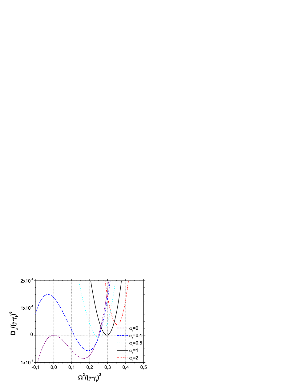
Figure 1:

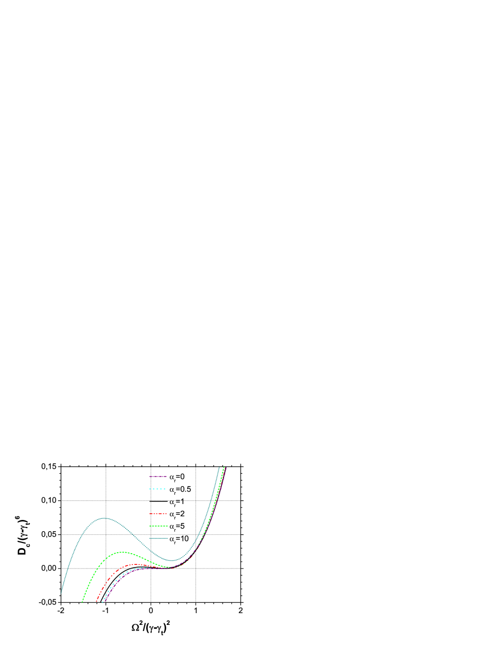
Figure 2:

Figure 3:

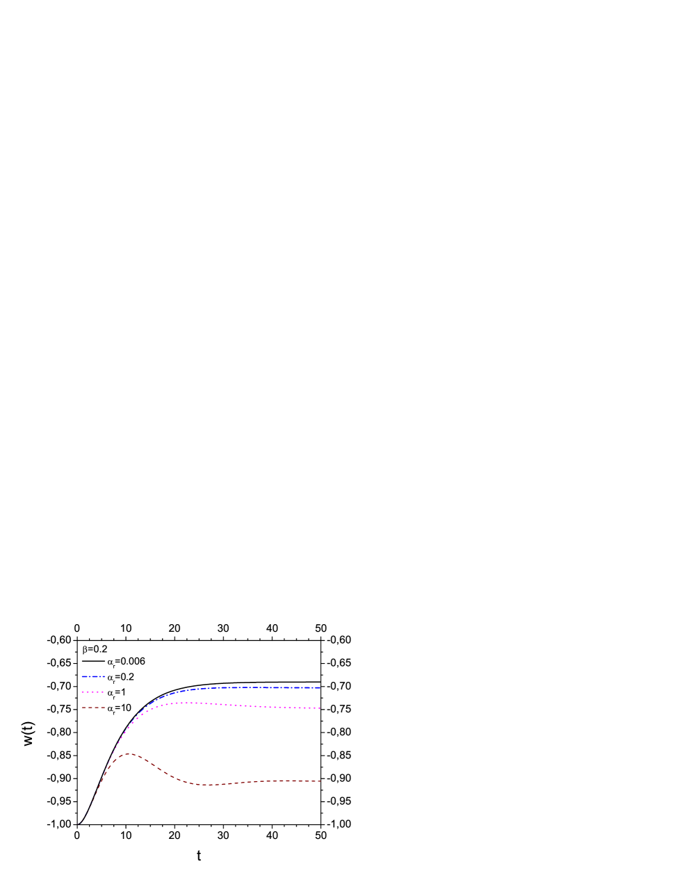
Figure 4:

References

- [1] F. Bloch, Nuclear induction, Phys. Rev. 70 (1946) 460-474.
- [2] H.C. Torrey, Transient nutations in nuclear magnetic resonance, Phys. Rev. 76 (1949) 1059-1068.
- [3] R.P. Feynman, F.L. Vernon, Jr., R.W. Hellwarth, Geometrical representation of the Schrödinger equation for solving maser problems, J. Appl. Phys. 28 (1957) 49-52.
- [4] P.J. Hore, K.A. McLauchlan, CIDEP and spin relaxation measurements by flash photolysis EPR methods, J. Magn. Reson. 36 (1979) 129-134.
- [5] P.K. Madhu, A. Kumar, Direct Cartesian-space solutions of generalized Bloch equations in the rotating frame, J. Magn. Reson. A 114 (1995) 201-211.
- [6] S.L. McCall, E.L. Hahn, Self-induced transparency, Phys. Rev. 183 (1969) 457-485.
- [7] J.H.-S. Wang, J.M. Levy, S.G. Kukolich, J.I. Steinfeld, Microwave transient nutation measurements of relaxation in OCS and NH3, Chem. Phys. 1 (1973) 141-148.
- [8] L. Allen, J.H. Eberly, Optical Resonance and Two-level Atoms, John Wiley & Sons, New York, 1975.
- [9] A. Yariv, Quantum Electronics, John Wiley & Sons, New York, 1975.
- [10] T. Basché, W.E. Moerner, M. Orrit, H. Talon, Photon antibunching in the fluorescence of a single dye molecule trapped in a solid, Phys. Rev. Lett. 69 (1992) 1516-1519.
- [11] C. Brunel, P. Tamarat, B. Lounis, J. Plantard, M. Orrit, Driving the Bloch vector of a single molecule: Towards a triggered single photon source, Comptes Rendus de l’Academie de Sciences - Serie IIb: Mecanique, Physique, Chimie, Astronomie 326 (1998) 911-918.
- [12] P. Tamarat, B. Lounis, J. Bernard, M. Orrit, S. Kummer, R. Kettner, S. Mais, T. Basché, Pump-probe experiments with a single molecule: ac-Stark effect and nonlinear optical response, Phys. Rev. Lett. 75 (1995) 1514-1517.
- [13] P. Tamarat, F. Jelezko, C. Brunel, A. Maali, B. Lounis, M. Orrit, Non-linear optical response of single molecules, Chem. Phys. 245 (1999) 121-132.
- [14] B. Butscher, J. Nipper, J.B. Balewski, L. Kukota, V. Bendkowsky, R. Löw, T. Pfau, Atom-molecule coherence for ultralong-range Rydberg dimers, Nature Physics 6 (2010) 970-974.
- [15] E.B. Flagg, A. Muller, J.W. Robertson, S. Founta, D.G. Deppe, M. Xiao, W. Ma, G.J. Salamo, C.K. Shih, Resonantly driven coherent oscillations in a solid-state quantum emitter, Nature Physics 5 (2009) 203-207.
- [16] S.K. Dutta et al, Multilevel effects in the Rabi oscillations of a Josephson phase qubit, Phys. Rev. B 78 (2008) 104510.
- [17] F. Jelezko, J. Wrachtrup, Single defect centres in diamond: A review, phys. stat. sol. (a) 203 (13) (2006) 3207-3225.
- [18] I. Aharonovich, S. Castelletto, D.A. Simpson, C.-H. Su, A.D. Greentree, and S. Prawer, Diamond-based single-photon emitters, Rep. Prog. Phys. 74 (2011) 076501.
- [19] J.M. Taylor, P. Cappellaro, L. Childress, L. Jiang, D. Budker, P.R. Hemmer, A. Yacoby, R. Walsworth, M.D. Lukin, High-sensitivity diamond magnetometer with nanoscale resolution, Nature Physics 4 (2008) 810-816.
- [20] J.R. Maze et al, Nanoscale magnetic sensing with an individual electronic spin in diamond, Nature 455 (2008) 644-647.
- [21] G. Balasubramanian et al, Nanoscale imaging magnetometry with diamond spins under ambient conditions, Nature 455 (2008) 648-651.
-
[22]
J.P. Hornak, The Basics of NMR.
Available online
http://www.cis.rit.edu/htbooks/nmr/inside.htm. -
[23]
A further information on the partial fraction decomposition
can be found on
http://en.wikipedia.org/wiki/Partial_fraction. -
[24]
A nice exposition of the Cardano’s formula and the
roots of a cubic polynomial can be found at
http://mathworld.wolfram.com/CubicFormula.htmlandhttp://en.wikipedia.org/wiki/Cubic_polynomial. - [25] A. Ekert, Girolamo Cardano - the gambling scholar, Phys. World, May 2009, 36-40.
- [26] A. Moroz, On a fully compensated formula for cubic roots (unpublished).
-
[27]
See for instance
http://en.wikipedia.org/wiki/Discriminant. - [28] H.-R. Noh, W. Jhe, Analytic solutions of the optical Bloch equations, Opt. Commun. 283 (2010) 2353-2355.
- [29] B. de Bartolo, Optical Interactions in Solids John Wiley & Sons, New York, 1968, pp. 431-442.
- [30] J. Bernard, L. Fleury, H. Talon, M. Orrit, Photon bunching in the fluorescence from single molecules: A probe for intersystem crossing, J. Chem. Phys. 98 (1993) 850-860.
- [31] H. de Vries, D.A. Wiersma, Fluorescence transient and optical free induction decay spectroscopy of pentacene in mixed crystals at K, J. Chem. Phys. 70 (1979) 5807-5823.
- [32] W. Magnus, On the exponential solution of differential equations for a linear operator, Commun. Pure Appl. Math. 7 (1954) 649-673.
- [33] F. Fer, Résolution de l’equation matricielle par produit infini d’exponentielles matricielles, Bull. Classe Sci. Acad. Roy. Bel. 44 (1958) 818-829.
- [34] P. Aniello, A new perturbative expansion of the time evolution operator associated with a quantum system, J. Opt. B: Quantum Semiclass. Opt. 7 (2005) S507-S522.
- [35] S. Blanes, F. Casas, J. A. Oteo, J. Ros, Magnus and Fer expansions for matrix differential equations: the convergence problem, J. Phys. A 31 (1998) 259-268.
-
[36]
A F77 code used to generate plots here is freely available at
http://www.wave-scattering.com/bloch.html