The generalized cusp in ABJ(M) $\mathbf{{\cal N}=6}$ Super Chern-Simons theories

Abstract

We construct a generalized cusped Wilson loop operator in ${\cal N}=6$ super Chern-Simons-matter theories which is locally invariant under half of the supercharges. It depends on two parameters and interpolates smoothly between the 1/2 BPS line or circle and a pair of antiparallel lines, representing a natural generalization of the quark-antiquark potential in ABJ(M) theories. For particular choices of the parameters we obtain 1/6 BPS configurations that, mapped on $S^{2}$ by a conformal transformation, realize a three-dimensional analogue of the wedge DGRT Wilson loop of ${\cal N}=4$. The cusp couples, in addition to the gauge and scalar fields of the theory, also to the fermions in the bi-fundamental representation of the $U(N)\times U(M)$ gauge group and its expectation value is expressed as the holonomy of a suitable super-connection. We discuss the definition of these observables in terms of traces and the role of the boundary conditions of fermions along the loop. We perform a complete two-loop analysis, obtaining an explicit result for the generalized cusp at the second non-trivial order, from which we read off the interaction potential between heavy 1/2 BPS particles in the ABJ(M) model. Our results open the possibility to explore in the three-dimensional case the connection between localization properties and integrability, recently advocated in $D=4$.

1 Introduction and results

The duality between string theory on asymptotically AdS spaces and conformal gauge theories, usually known as the AdS/CFT correspondence, has experienced an important evolution in the last few years. General non-BPS observables, as anomalous dimensions of composite operators and scattering amplitudes, can now be studied at high precision level providing sophisticated tests of the correspondence and sometimes offering non-trivial interpolating functions between weak and strong coupling. In both cases, the underlying integrability properties of the planar theory play a crucial role in the exact quantum evaluation and allow to follow the transition between the opposite regimes. Dramatic progresses have also concerned more traditional investigations, as the study of protected sectors of supersymmetric gauge theories: the introduction of powerful localization techniques makes now possible the exact computation of complicated path-integrals, providing again examples of interpolation between perturbative and asymptotic behaviors. It is tempting to speculate if the two different approaches, integrability and localization, could be somehow connected, at least in the computation of specific observables.

This evocative possibility has been vigorously advocated in Drukker:2011za for a general class of Wilson loops in $\mathcal{N}=4$ super Yang-Mills theory and concretely realized in a series of recent papers Correa:2012at ; Correa:2012nk ; Drukker:2012de ; Correa:2012hh , where a new set of integral equations of TBA type, describing exactly a generalized cusp anomalous dimension, have been derived and checked against localization and perturbation theory at three loops. The result is striking and it contains, in principle, the all-order expression of the static potential between two heavy charged particles in four-dimensional maximally supersymmetric gauge theory.

Wilson loops are important observables in nonabelian gauge theories: they compute the potential between heavy colored probes, representing an order parameter for confinement Wilson:1974sk and encode a large part of information of the high-energy scattering between charged particles Korchemsky:1988si ; Korchemsky:1992xv . In ${\cal N}=4$ super Yang-Mills theory they play a prominent role, being the observables directly related to the fundamental string of the dual theory in $AdS_{5}\times S^{5}$ Rey:1998ik ; Maldacena:1998im . They are conjectured to calculate scattering amplitudes exactly Bern:2005iz ; Alday:2007hr and in particular cases they are BPS operators Dymarsky:2009si ; Cardinali:2012sy , whose quantum expectation value can be derived for any strength of the coupling constant Erickson:2000af ; Drukker:2000rr ; Pestun:2007rz . In Drukker:2011za a two-parameters family of Wilson loops in ${\cal N}=4$ SYM has been proposed and studied both at weak and strong coupling: it consists of two rays in $\mathbb{R}^{4}$ meeting at a point, with a cusp angle denoted by $\pi-\varphi$. Because the Maldacena-Wilson loops in ${\cal N}=4$ SYM couple to a real scalar field, it is natural to consider different scalars on different rays, connected by an $R$-symmetry rotation of parameter $\theta$. By varying continuously $\varphi$ and $\theta$ and performing suitable conformal transformations, these observables can be related to important physical quantities and to interesting BPS configurations. Mapping the theory to $S^{3}\times\mathbb{R}$ one obtains a pair of antiparallel lines, separated by angle $\pi-\varphi$ on the sphere, and derives the potential $V(\lambda,\varphi,\theta)$ between two heavy $W$-bosons propagating over a large time $T$:

$$\langle\mathcal{W}_{\rm lines}\rangle\simeq\exp\left(-TV(\lambda,\varphi,\theta)\right).$$ (1)

The usual potential in the flat space is easily recovered by taking the residue of $V(\lambda,\varphi,0)$ as $\varphi\to\pi$ Drukker:2011za . In the cusped version, the Wilson loop has the leading form

$$\langle\mathcal{W}_{\rm cusp}\rangle\simeq\exp\left(-\Gamma_{cusp}(\lambda,\varphi,\theta)\log\left(\frac{\Lambda}{\epsilon}\right)\right),$$ (2)

and it turns out that $\Gamma_{cusp}(\lambda,\varphi,\theta)=V(\lambda,\varphi,\theta)$, with $\Lambda$ and $\epsilon$ being IR and UV cut-offs respectively Polyakov:1980ca ; Brandt:1981kf . The cusped Wilson loops are strictly related to scattering amplitudes in Minkowski space: taking $\varphi$ imaginary and large, $\varphi=i\phi$, produces to the so-called universal cusp anomalous dimension $\gamma_{cusp}(\lambda)$ Korchemsky:1987wg

$$\lim_{\phi\to\infty}\Gamma_{cusp}(\lambda,i\varphi,\theta)=\frac{\varphi\,\gamma_{cusp}(\lambda)}{4}.$$ (3)

Remarkably BPS configurations are also included in the family: for $\theta=\pm\varphi$ the cusped Wilson loop is of Zarembo’s type Zarembo:2002an , implying the vanishing of $\Gamma_{cusp}(\lambda,\varphi,\theta)$ in this case. By mapping conformally the rays into $S^{2}$ we recover instead the DGRT wedge, a well studied 1/4 BPS operator Drukker:2007qr ; Bassetto:2008yf ; Young:2008ed belonging to the general class of loops on $S^{3}$ introduced in Drukker:2007qr . The quantum expectation value of the wedge is computed exactly by pertturbative two-dimensional Yang-Mills theory Bassetto:1998sr , a property shared with other DGRT loops on $S^{2}$ Pestun:2009nn and with a certain class of loop correlators Bassetto:2009rt ; Bassetto:2009ms ; Giombi:2009ds ; Giombi:2012ep . We remark that path-integral localization properties are essential in order to derive these results.

In the limit of small $\varphi$, $\Gamma_{cusp}(\lambda,\varphi,0)\simeq-B(\lambda)\varphi^{2}$ computes also the radiation of a particle moving along an arbitrary smooth path Correa:2012at and an exact expression can be obtained by exploiting the BPS properties at $\varphi=0$. A simple modification applies as well in expanding around the general BPS points $\theta=\pm\varphi$, thanks to the knowledge of the all-orders expression of the DGRT wedge. Further, in Drukker:2012de ; Correa:2012hh , a powerful set of TBA type integral equations for the generalized cusp was derived, using integrability: the explicit one-loop perturbative result Drukker:2012de and the three-loop expression of the near BPS limit Correa:2012nk were recovered as a check of the procedure.

In view of these recent and exciting developments, it appears natural to wonder wether similar results could also be obtained for other superconformal gauge theories with integrable structures: the obvious choice is to investigate what happens in ${\cal N}=6$ super Chern-Simons theories with matter, also known as ABJ(M) Aharony:2008ug ; Aharony:2008gk . Wilson loops in ABJ(M) theory are still a rather unexplored subject: equivalence with scattering amplitudes has been shown at the second order in perturbation theory Henn:2010ps ; Chen:2011vv ; Bianchi:2011dg ; Bianchi:2011fc and a quite mysterious functional similarity with their four-dimensional cousins seems to emerge. On the other hand, supersymmetric configurations, supported on straight lines and circles, have been discovered Drukker:2009hy ; Drukker:2008zx ; Chen:2008bp ; Rey:2008bh and a localization formula, reducing the computation to an explicit matrix model average, has been derived Kapustin:2009kz . Concrete results at weak and strong coupling, using matrix model and topological string techniques, are presented in a beautiful series of papers Marino:2009jd ; Drukker:2010nc ; Drukker:2011zy ; Marino:2011eh , where also various aspects of the partition function on $S^{3}$ have been discussed. Nevertheless many issues should be understood in order to extend the generalized cusp program. First of all it does not even exist a computation of the standard quark-antiquark potential nor of the conventional cusped Wilson loop. Secondly, BPS lines and circles appear in two fashions, distinguished by the degree of preserved supersymmetry: we have the 1/6 BPS operators, originally defined in Drukker:2008zx ; Chen:2008bp (see also Rey:2008bh ), that are a straightforward extension of the Maldacena-Wilson loop to the three-dimensional case. The (quadratic) coupling with the scalar fields of the theory is governed by a mass matrix $M^{I}_{J}$, preserving an $SU(2)\times SU(2)$ of the original $R$-symmetry, while gauge fields appear in the usual way. Although its simplicity, this kind of loop cannot be considered the dual of the fundamental string living in $AdS_{4}\times\mathbb{CP}^{3}$, because supersymmetries do not match Drukker:2008zx . The field theoretical partner of the fundamental string is instead the 1/2 BPS loop discovered in Drukker:2009hy (see Lee:2010hk for a derivation arising from the low-energy dynamics of heavy $W$-bosons): the loop couples, in addition to the gauge and scalar fields of the theory, also to the fermions in the bi-fundamental representation of the $U(N)\times U(M)$ gauge group. These ingredients are combined into a superconnection whose holonomy gives the Wilson loop, which can be defined for any representation of the supergroup $U(N|M)$. Supersymmetry is realized through a highly sophisticated mechanism, as a super-gauge transformation, requiring therefore the full non-linear structure of the path-ordering. Actually both loops turn out to be in the same cohomology class, differing by a BRST exact term with respect the localization complex: their quantum expectation value should be therefore the same Drukker:2009hy . The above equivalence has not been checked at weak-coupling, where perturbative computations have been performed just for the 1/6 BPS circle Drukker:2008zx ; Chen:2008bp ; Rey:2008bh , the presence of fermions complicates the calculations and rises delicate issues on the regularization procedure. Crucially there are also no examples of loops with fewer supersymmetries, including the known BPS lines and circle as particular cases: it would be interesting to find configurations of this type that could also help to understand better the mysterious cohomological equivalence.

This paper represents a first step towards a systematic study of generalized cusps in ABJ(M) theories: similar configurations have been discussed, at strong coupling, in Forini:2012bb . We hope that our investigations could stimulate the application of integrability and cohomological techniques in the exact evaluation of non-BPS observables, such as the heavy-bosons static potential. Our main concern here is the construction of a generalized cusp using two 1/2 BPS rays, the study of its supersymmetric properties and its quantum behavior at weak-coupling. The additional $R$-symmetry deformation is obtained by preserving different $SU(3)$ subgroups on the two lines: from the bosonic point of view this amounts to deform the mass-matrix $M^{I}_{J}$, by rotating two directions of opposite eigenvalues. The fermionic couplings experience a similar deformation and are also explicitly affected by the geometric parameter $\varphi$, because they transform as spinors under spatial rotations. We study the supersymmetry shared by the two rays and we discover that for $\theta=\pm\varphi$ two charges are still globally preserved: in this case the super-gauge transformations, encoding the supersymmetry variation on the two edges of the cusp, become smoothly connected at the meeting point. A key observation made in the original paper of Drukker and Trancanelli Drukker:2009hy was that, for the 1/2 BPS circle, only the trace of the super-holonomy turns out to be supersymmetric invariant and not its super-trace. Conversely the fermionic couplings were assumed to be anti-periodic on the loop: here we examine the same problem on the new BPS configurations. By performing an explicit conformal transformation, we map our cusp on $S^{2}$, obtaining a wedge: the fermionic couplings, constant on the plane, become space-dependent as an effect of the conformal map, and connected by a non-trivial rotation on the upper point of the wedge. In the BPS case this matrix simply appears as an anti-periodicity, and therefore it is again the trace that leads to supersymmetric invariance. The loops constructed in this way are a sort of ABJ(M) version of the DGRT wedge Drukker:2007qr and preserve 1/6 of the original supersymmetries. We consistently define our generalized cusp as the trace of the super-holonomy and attempt the computation of its quantum expectation value in perturbation theory. We observe two basic differences with the analogous four-dimensional computation performed in Drukker:2011za : first of all the effective propagators here, attaching on one side of the cusp only, are not automatically vanishing, as it happens for ${\cal N}=4$ SYM in Feynman gauge, and the fermionic sector gives a divergent contribution at one-loop, that has to be regularized and renormalized. Secondly, because of the presence of a supergroup structure, involving fermions coupled to the external lines, it is not obvious to extend the non-abelian exponentiation theorem to this setting: we could not rely on such powerful device to reduce the amount of computations and to properly isolate the cusp anomalous dimensions. Concerning this second point we make the natural assumption that our cusped loops undergo through a “double-exponentiation”

$$\mathcal{W}=\frac{M\exp(V_{N})+N\exp(V_{M})}{N+M},$$ (4)

where the generalized potentials $V_{N}$ and $V_{M}$ are simply related by exchanging $N$ with $M$. A highly non-trivial check of the above assumption is the actual exponentiation of the one-loop term, constraining in particular the structure of the double-poles (in the dimensional regularization parameter $\epsilon=(3-D)/2$) appearing at two-loops. We find a perfect agreement of our results with the double-exponentiation hypothesis, recovering at the second order in perturbation theory the quadratic contributions coming from the first order one. Our final expression for the unrenormalized $V_{N}$ is

$$V_{N}= \left(\frac{2\pi}{\kappa}\right)N\left(\frac{\Gamma(\frac{1}{2}-\epsilon)}{4\pi^{3/2-\epsilon}}\right)(\mu L)^{2\epsilon}\left[\frac{1}{\epsilon}\left(\frac{\cos\frac{\theta}{2}}{\cos\frac{\varphi}{2}}-2\right)-2\frac{\cos\frac{\theta}{2}}{\cos\frac{\varphi}{2}}\log\left(\sec\left(\frac{\varphi}{2}\right)+1\right)\right]+$$

$$\left(\frac{2\pi}{\kappa}\right)^{\!\!2}N^{2}\!\left(\frac{\Gamma\!\left(\frac{1}{2}-\epsilon\right)}{4\pi^{3/2-\epsilon}}\right)^{2}(\mu L)^{4\epsilon}\left[\frac{1}{\epsilon}\log\left(\cos\frac{\varphi}{2}\right)^{2}\left(\frac{\cos\frac{\theta}{2}}{\cos\frac{\varphi}{2}}-1\right)+O(1)\right].$$ (5)

Here $k$ is the Chern-Simons level, $L$ is the length of the lines and $\mu$ is the renormalization scale introduced by dimensional regularization. To extract the cusp anomalous dimension we have to carefully subtract the divergences coming from single-leg diagrams: for closed contours in four dimensions these are usually associated, in a generic gauge theory, to a linear divergence proportional to the perimeter loop Polyakov:1980ca . In the smooth case once subtracted this perimeter term. the standard lagrangian renormalization makes the quantum expectation value finite Brandt:1981kf ; Exp .

When open contours are considered the situation changes and some subtleties in the renormalization procedure arise: a systematic analysis of these problems have been performed in eighties Aoyama:1981ev ; Dorn1 ; Dorn2 ; Knauss:1984rx ; Dorn:1986dt and (somehow) forgotten. The outcome is essentially contained in the introduction of a further a gauge-dependent renormalization constant, sometimes called $Z_{\rm open}$, taking into account shape-independent extra-divergencies associated to the end-points of the contour. To isolate the true gauge-invariant cusp-divergence these spurious contributions should be subtracted because, in general, they appear for finite lenght of the lines. ${\cal N}=4$ SYM in Feynman gauge represents a lucky situation in which, due to the peculiar combination of the gauge/scalar propagator, these additional effects are not present. We remark that in general $\alpha$-gauge a $Z_{\rm open}$ should be taken into account. We will carefully review all these topics in subsec. 6.2.

In three dimensions the superconformal case, due to the fermionic couplings, inevitably implies the appearence of the spurios single-length contributions: we will carefully discuss the subtraction procedure, examing in details the paradigmatic case of the 1/2 BPS infinite-line, and we hope to clarify the structure of the divergences for these family of loops. We will also comment on the difference between the 1/2 BPS and 1/6 BPS cases, showing that at finite-length the cohomological equivalence is broken by boundary terms, generating the unexpected divergence at quantum level.

Our final receipt amounts to subtract, in the second order computation, the one-loop poles associated to single line diagrams, normalizing in this way the final result to the straight line, 1/2 BPS contour

$$\!\!V^{\rm Ren.}_{N}= \left(\frac{2\pi}{\kappa}\right)N\left(\frac{\Gamma(\frac{1}{2}-\epsilon)}{4\pi^{3/2-\epsilon}}\right)\!(\mu L)^{2\epsilon}\!\!\left[\frac{1}{\epsilon}\left(\frac{\cos\frac{\theta}{2}}{\cos\frac{\varphi}{2}}-1\right)\!\!-2\frac{\cos\frac{\theta}{2}}{\cos\frac{\varphi}{2}}\log\left(\sec\left(\frac{\varphi}{2}\right)\!+\!1\right)\!\!+\log 4\right]\!+$$

$$+\left(\frac{2\pi}{\kappa}\right)^{\!\!2}N^{2}\!\left(\frac{\Gamma\!\left(\frac{1}{2}-\epsilon\right)}{4\pi^{3/2-\epsilon}}\right)^{2}(\mu L)^{4\epsilon}\left[\frac{1}{\epsilon}\log\left(\cos\frac{\varphi}{2}\right)^{2}\left(\frac{\cos\frac{\theta}{2}}{\cos\frac{\varphi}{2}}-1\right)+O(1)\right].$$ (6)

From the above expression we can easily recover the quark-antiquark potential, taking the limit $\varphi\to\pi$ and following the prescription of Drukker:2011za

$$V^{(s)}_{N}(R)=\frac{N}{k}\frac{1}{R}-\left(\frac{N}{k}\right)^{2}\frac{1}{R}\log\left(\frac{T}{R}\right).$$ (7)

We find a logarithmic, non-analytic term in $T/R$ at the second non-trivial order that, as in four dimensions, is expected to disappear when resummation of the perturbative series is performed. In the opposite limit, for large imaginary $\varphi$, we get the universal cusp anomaly (using the four-dimensional definition)

$$\gamma_{cusp}=\frac{N^{2}}{k^{2}},$$ (8)

reproducing the result obtained directly from the light-like cusp Henn:2010ps .

The plan of the paper is the following: in Section 2 we review the construction of 1/2 BPS Wilson lines in ABJ models, giving us the possibility to introduce the peculiar structures entailed by maximal supersymmetric loops in ${\cal N}=6$ super Chern-Simons-matter theories. Section 3 is devoted to the explicit realization of the generalized cusp: we obtain the appropriate bosonic and fermionic couplings and their deformations and discuss how the supersymmetry properties depends on the relevant parameters. The conformal transformation, mapping the cusp on a wedge of $S^{2}$, is also presented: the periodicity properties of the fermions are derived and BPS observables are obtained taking the trace of the super-holonomy. In Section 4 we start the quantum investigation computing the expectation value at the first order in perturbation theory. The two-loop analysis is contained in Section 5. The final result, obtained by summing up all the contributions and performing the renormalization procedure is presented in Section 6, where the peculiar divergences structure of these observables is carefully discussed. We present a rather detailed review of known facts on the renormalization of closed, open and cusped Wilson loops, that we think will clarify the apparent intricacy of our subtraction procedure and unveil its gauge-independent meaning. Some conclusions and outlooks appear in Section 7. We complete the paper with some appendices, containing our conventions and the technical details of the computations.

2 1/2 BPS straight-line in ABJ theories

We start by reviewing the construction of the $1/2-$BPS Wilson line given in Drukker:2009hy ; Lee:2010hk : the mechanism leading to its gauge invariance is carefully reconsidered, since it is substantially different from the four dimensional analogue.

The central idea of Drukker:2009hy is to replace the obvious $U(N)\times U(M)$ gauge connection with a super-connection

$$\mathcal{L}(\tau)\equiv-i\begin{pmatrix}i\mathcal{A}&\sqrt{\frac{2\pi}{k}}|\dot{x}|\eta_{I}\bar{\psi}^{I}\\ \sqrt{\frac{2\pi}{k}}|\dot{x}|\psi_{I}\bar{\eta}^{I}&i\hat{\mathcal{A}}\end{pmatrix}\ \ \ \ \mathrm{with}\ \ \ \ \left\{\begin{matrix}\mathcal{A}\equiv A_{\mu}\dot{x}^{\mu}-\frac{2\pi i}{k}|\dot{x}|M_{J}^{\ \ I}C_{I}\bar{C}^{J}\\ \\ \hat{\mathcal{A}}\equiv\hat{A}_{\mu}\dot{x}^{\mu}-\frac{2\pi i}{k}|\dot{x}|\hat{M}_{J}^{\ \ I}\bar{C}^{J}C_{I},\end{matrix}\ \right.$$ (9)

belonging to the super-algebra of $U(N|M)$. In (9) the coordinates $x^{\mu}(\tau)$ draw the contour along which the loop operator is defined, while $M_{J}^{\ \ I}$, $\hat{M}_{J}^{\ \ I}$, $\eta_{I}^{\alpha}$ and $\bar{\eta}^{I}_{\alpha}$ are free parameters. The latter two, in particular, are Grassmann even quantities even though they transform in the spinor representation of the Lorentz group.

The dependence of $\mathcal{L}(\tau)$ on the fields is largely dictated by dimensional analysis and transformation properties. Since the classical dimension of the scalars in $D=3$ is $1/2$, they could only appear as bilinears, transforming in the adjoint and thus entering in the diagonal blocks together with the gauge fields. Instead the fermions have dimension $1$ and should appear linearly. Since they transform in the bi-fundamentals of the gauge group, they are naturally placed in the off-diagonal entries of the matrix (9).

When the contour $x^{\mu}(\tau)$ is a straight-line $S$, the invariance under translations along the direction defined by $S$ ensures that all the couplings can be chosen to be independent of $\tau$, i.e. constant. Moreover the requirement of having an unbroken $SU(3)$ $R-$symmetry, as that of the dual string configuration, restricts the couplings $M_{J}^{\ \ I}$,  $\hat{M}_{J}^{\ \ I}$, $\eta_{I}^{\alpha}$  and  $\bar{\eta}^{I}_{\alpha}$ to be of the form

$$\begin{split}\eta_{I}^{\alpha}=n_{I}\eta^{\alpha},\ \ \ \ \bar{\eta}^{I}_{\alpha}=\bar{n}^{I}\bar{\eta}_{\alpha},\ \ \ \ M_{J}^{\ \ I}=p_{1}\delta^{I}_{J}-2p_{2}n_{J}\bar{n}^{I},\ \ \ \ \widehat{M}_{J}^{\ \ I}=q_{1}\delta^{I}_{J}-2q_{2}n_{J}\bar{n}^{I}.\end{split}$$ (10)

Here $n_{I}$ and $\bar{n}^{I}$ are two complex conjugated vectors which transform in the fundamental and anti-fundamental representation and determine the embedding of the $SU(3)$ subgroup in $SU(4)$. By rescaling $\eta^{\alpha}$ and $\bar{\eta}_{\alpha}$, we can always choose $n_{I}\bar{n}^{I}=1$. The parameters $p_{i}$ and $q_{i}$ in the definition of $M$ and $\hat{M}$ instead control the eigenvalues of the two matrices.

The free parameters appearing in (10) can be then constrained by imposing that the resulting Wilson loop is globally supersymmetric. This issue is subtle: the usual requirement $\delta_{\rm susy}\mathcal{L}(\tau)=0$ does not yield any 1/2 BPS solution indeed. We just obtain loop operators which are merely bosonic ($\eta=\bar{\eta}=0$) and at most $1/6$ BPS Drukker:2008zx ; Rey:2008bh . In order to obtain 1/2 BPS solution, we must replace $\delta_{\rm susy}\mathcal{L}(\tau)=0$ with the weaker condition Drukker:2009hy ; Lee:2010hk

$$\delta_{\rm susy}\mathcal{L}(\tau)=\mathfrak{D}_{\tau}G\equiv\partial_{\tau}G+i\{\mathcal{L},G],$$ (11)

where the r.h.s. is the super-covariant derivative constructed out of the connection $\mathcal{L}(\tau)$ acting on a super-matrix $G$ in $\mathfrak{u}(N|M)$. The requirement (11) assures that the action of the relevant supersymmetry charges translates into an infinitesimal super-gauge transformation for $\mathcal{L}(\tau)$ and thus the “traced” loop operator is invariant.

Now we shall recapitulate the analysis of Drukker:2009hy leading to fix the free parameters in (10). However, for future convenience, we shall present the result in a covariant notation i.e. without referring to a specific form of the straight line.

We start by considering the structure of the infinitesimal gauge parameter in (11). Since the supersymmetry transformation of the bosonic fields does not contain any derivative of the fields, the super-matrix $G$ in (11) must be anti-diagonal

$$G=\begin{pmatrix}0&g_{1}\\ \bar{g}_{2}&0\end{pmatrix}\ \ \Rightarrow\ \ \mathfrak{D}_{\tau}G=\begin{pmatrix}\sqrt{\frac{2\pi}{k}}|\dot{x}|(\eta_{I}\bar{\psi}^{I}\bar{g}_{2}+g_{1}\psi_{I}\bar{\eta}^{I})&\mathcal{D}_{\tau}g_{1}\\ \mathcal{D}_{\tau}\bar{g}_{2}&\sqrt{\frac{2\pi}{k}}|\dot{x}|(\bar{g}_{2}\eta_{I}\bar{\psi}^{I}+\psi_{I}\bar{\eta}^{I}g_{1})\end{pmatrix}.$$ (12)

Here $\mathcal{D}_{\tau}$ is the covariant derivative constructed out of the dressed bosonic connections $\mathcal{A}$ and $\hat{\mathcal{A}}$ and given by

$$\mathcal{D}_{\tau}g_{1} =\partial_{\tau}g_{1}+i(\mathcal{A}\,g_{1}-g_{1}\,\hat{\mathcal{A}})\,,\ \ \ \ \mathcal{D}_{\tau}\bar{g}_{2} =\partial_{\tau}\bar{g}_{2}-i(\bar{g}_{2}\,\mathcal{A}-\hat{\mathcal{A}}\,{\bar{g}}_{2}).$$ (13)

The condition (11) for the anti-diagonal entries first constrains the form of the spinor $\eta$ and $\bar{\eta}$ to obey the two conditions

$${(\dot{x}^{\mu}\gamma_{\mu})_{\alpha}^{\ \ \beta}}=\frac{1}{(\eta\bar{\eta})}|\dot{x}|(\eta^{\beta}\bar{\eta}_{\alpha}+\eta_{\alpha}\bar{\eta}^{\beta})\ \ \ \ \ \ (\eta^{\beta}\bar{\eta}_{\alpha}-\eta_{\alpha}\bar{\eta}^{\beta})=(\eta\bar{\eta})\delta^{\beta}_{\alpha},$$ (14)

which assure that the covariant derivatives appearing in the supersymmetry transformations of $\psi\bar{\eta}$ and $\eta\bar{\psi}$ are only evaluated along the circuit. The value of the parameters $p_{i}$ and $q_{i}$, appearing in the matrices $M$ and $\hat{M}$, is equal to $1$ for the same reason.

The requirement (11) for the diagonal entries does not yield, instead, new conditions, simply fixing the normalization

$$\eta\bar{\eta}=2i.$$ (15)

In particular the vector $n_{I}$ continues to be unconstrained.

The origin of the superconnection was also investigated from the point of view of the low-energy dynamics of heavy “W-bosons” in Lee:2010hk . It was shown that when the theory is higgsed preserving half of the total supersymmetry, the corresponding low-energy Lagrangian enjoys a larger gauge invariance, given by the supergroup $U(N|M)$. The light fermions do not decouple from the dynamics, at variance with the case of ${\cal N}=4$ SYM, and their interactions with heavy $W$-bosons are described by $\eta_{I}^{\alpha},\bar{\eta}^{I}_{\alpha}$. The role of the mass-matrix is instead played by $M_{J}^{\ \ I},\widehat{M}_{J}^{\ \ I}$. This result unveils the physical nature of the potential related to the rectangular Wilson loops, constructed with 1/2 BPS lines in ABJ(M) theories.

Armed with the explicit form for the couplings, we can find twelve supercharges Drukker:2009hy whose action on $\mathcal{L}(\tau)$ can be cast into the form (11). There are six supercharges of the Poincarè type,

$$\bar{\theta}^{IJ\beta}=(\bar{\eta}^{I\beta}\bar{v}^{J}-\bar{\eta}^{J\beta}\bar{v}^{I})-i\epsilon^{IJKL}\eta_{K}^{\beta}u_{L}=(\bar{n}^{I}\bar{v}^{J}-\bar{n}^{J}\bar{v}^{I})\bar{\eta}^{\beta}-i\epsilon^{IJKL}n_{K}u_{L}\eta^{\beta},$$ (16)

parametrized by two vectors $u^{I}$ and $\bar{v}^{I}$ that satisfy $(n_{I}\bar{v}^{I})=(\bar{n}^{I}u_{I})=0$. We remark that these vectors are really independent in Euclidean signature, while $\bar{v}^{I}=u_{I}^{\dagger}$ as a result of the reality conditions present in the Minkowski case. Next to the above $\bar{\theta}^{IJ}$ we can also identify six super-conformal charges $\bar{\vartheta}^{IJ\beta}$, whose structure is again given by an expansion of the form (16). The origin of this second set of supersymmetries is easily understood: they are obtained by combining the Poincarè supercharges (16) with a special conformal transformation in the direction associated to the straight-line.

The analysis presented in Drukker:2009hy ; Lee:2010hk also provides the explicit form of the gauge function in terms of the scalar fields, the spinor couplings and the supersymmetry parameters $\bar{\theta}^{IJ}$. In our notation, they take the form

$$g_{1}=2\sqrt{\frac{2\pi}{k}}n_{K}(\eta\bar{\theta}^{KL})C_{L}\ \ \ \ \ \ \mathrm{and}\ \ \ \ \ \ \ \bar{g}_{2}=-\sqrt{\frac{2\pi}{k}}\varepsilon_{IJKL}\bar{n}^{K}(\bar{\theta}^{IJ}\bar{\eta})\bar{C}^{L}.$$ (17)

Now we come back to analyze the issue of supersymmetry invariance for a generic Wilson loop defined by (9) when its variation can be cast into the form (11). The finite transformation of the untraced operator

$$W(\tau_{1},\tau_{0})=\mathrm{P}\exp\left(-i\int_{\tau_{0}}^{\tau_{1}}d\tau\mathcal{L}(\tau)\right),$$ (18)

under the gauge transformation generated by $G(\tau)$ in (12), can be written as Lee:2010hk

$$W(\tau_{1},\tau_{0})\mapsto U^{-1}(\tau_{1})W(\tau_{1},\tau_{0})U(\tau_{0}),$$ (19)

where $U(\tau)=e^{iG(\tau)}$. For a closed path $\gamma$ $[\gamma(\tau_{0})=\gamma(\tau_{1})]$, we must carefully consider the boundary conditions obeyed by the gauge functions $g_{1}$ and $\bar{g}_{2}$ in order to define the gauge invariant operator. If they are periodic, i.e. $g_{1}(\tau_{0})=g_{1}(\tau_{1})$ and $\bar{g}_{2}(\tau_{0})=\bar{g}_{2}(\tau_{1})$, we find that $U(\tau_{0})=U(\tau_{1})$ and a gauge invariant operator is obtained by taking the usual super-trace

$$\mathcal{W}=\mathrm{Str}(W).$$ (20)

Actually it is the super-trace to be invariant under similitude transformations. However we can have different situations: in Drukker:2009hy it was examined another 1/2-BPS loop, the circle, and pointed out that the function $g_{1}$ and $\bar{g}_{2}$ are anti-periodic in this case. Consequently the untraced operator, because $U(\tau_{1})=U^{-1}(\tau_{0})$, transforms as follows

$$W(\tau_{1},\tau_{0})\mapsto U(\tau_{0})W(\tau_{1},\tau_{0})U(\tau_{0}).$$ (21)

To construct a supersymmetric operator, we first observe that

$$\mbox{\scriptsize$\begin{pmatrix}\mathds{1}&0\\ 0&-\mathds{1}\end{pmatrix}$}U(\tau_{0})\mbox{\scriptsize$\begin{pmatrix}\mathds{1}&0\\ 0&-\mathds{1}\end{pmatrix}$}=U^{-1}(\tau_{0})$$ (22)

for a gauge transformation generated by the matrix $G$ in (12). Then the operator

$$\mathcal{W}=\mathrm{Str}\left[\mbox{\footnotesize$\begin{pmatrix}\mathds{1}&0\\ 0&-\mathds{1}\end{pmatrix}$}\mbox{$\displaystyle\mathrm{P}\!\exp\left(-i\int_{\tau_{0}}^{\tau_{1}}d\tau\mathcal{L}(\tau)\right)$}\right]\equiv\mathrm{Tr}\left[\mbox{$\displaystyle\mathrm{P}\!\exp\left(-i\int_{\tau_{0}}^{\tau_{1}}d\tau\mathcal{L}(\tau)\right)$}\right]$$ (23)

turns out to be invariant. In the case of a straight line the situation is more intricate, since we deal with an open infinite circuit. The invariance under supersymmetry is recovered by choosing a set of suitable boundary conditions for the fields, in particular for the scalars appearing in the definition of $g_{1}$ and $\bar{g}_{2}$. The naive statement that they must vanish when $\tau=\pm\infty$ seems to leave open a double possibility for defining a supersymmetric operator

$$\begin{split}\mathcal{W}_{-}=&\frac{1}{N-M}\mathrm{Str}\left[\mbox{$\displaystyle\mathrm{P}\!\exp\left(-i\int_{\tau_{0}}^{\tau_{1}}d\tau\mathcal{L}(\tau)\right)$}\right]\ {\mathrm{or}}\\ \mathcal{W_{+}}=&\frac{1}{N+M}\mathrm{Tr}\left[\mbox{$\displaystyle\mathrm{P}\!\exp\left(-i\int_{\tau_{0}}^{\tau_{1}}d\tau\mathcal{L}(\tau)\right)$}\right],\end{split}$$ (24)

since $U(\pm\infty)=\mathds{1}$ and $W(\tau_{1},\tau_{0})$ itself is invariant. We shall consider in our explicit quantum computation the second possibility: as we will see, the trace is the correct option to generate BPS observables from closed contours, connected to ours through conformal transformations. It also seems to provide a result consistent with the interpretation of the Wilson loop in terms of quark-antiquark potentials.

3 The generalized cusp

We discuss here in detail the Wilson loop observables we will study in the rest of the paper. After constructing the bosonic and fermionic couplings for the generalized cusp, we study the possibility to find novel BPS configurations. We determine the BPS conditions for the cusp parameters and derive the explict form of the related supercharges. Finally we map our new configurations on the sphere $S^{2}$, by means of conformal transformations, and we obtain a non-trivial BPS deformation of the BPS circle constructed in Drukker:2009hy .

3.1 Bosonic and fermionic couplings

We start by considering the theory on the Euclidean space-time. We shall consider two rays in the plane $(1,2)$ intersecting at the origin as illustrated in fig. 1. The angle between the rays is $\pi-\varphi$, such that for $\varphi=0$ they form a continuous straight line. The path in fig. 1 is given by

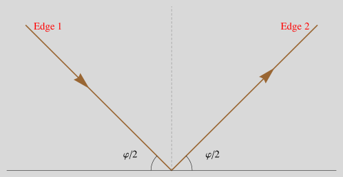
Figure 1: Eq. (25) represents a planar cusp, whose angular extension is given by $\pi-\varphi$.

$$x^{0}=0\ \ \ \ \ x^{1}=s\cos\frac{\varphi}{2}\ \ \ \ \ x^{2}=|s|\sin\frac{\varphi}{2}\ \ \ \ \ -\infty\leq s\leq\infty.$$ (25)

The fermionic couplings on each straight-line possess the factorized structure discussed in the previous section, i.e.

$$\eta_{iM}^{\alpha}=n_{iM}\eta^{\alpha}\ \ \ \ \ \mathrm{and}\ \ \ \ \ \bar{\eta}^{M}_{i\alpha}=\bar{n}_{i}^{M}\bar{\eta}_{i\alpha}.$$ (26)

The additional index $i=1,2$ in (26) specifies which edge of the cusp we are considering. For $i=\mathrm{1}$, $\eta_{1\alpha}$ is constructed as the eigenspinor of eigenvalue $1$ of the matrix $\frac{\dot{x}_{1}^{\mu}}{|\dot{x}_{1}|}\gamma_{\mu}$:

$$\frac{\dot{x}_{1}^{\mu}}{|\dot{x}_{1}|}\gamma_{\mu}\bar{\eta}_{1}=\left(\cos\frac{\varphi}{2}\gamma_{1}-\sin\frac{\varphi}{2}\gamma_{2}\right)\bar{\eta}_{1}=\bar{\eta}_{1}\ \ \ \ \Rightarrow\ \ \ \ \bar{\eta}_{1\alpha}=i\begin{pmatrix}e^{i\frac{\varphi}{4}}\\ e^{-i\frac{\varphi}{4}}\end{pmatrix}$$ (27)

as a result of the two constraints (14). Similarly the spinor $\eta_{1}^{\alpha}$ obeys the hermitian conjugate of the above equation and thus $\eta_{1}^{\alpha}\propto(\bar{\eta}_{1\alpha})^{\dagger}$. The condition (15) fixes the relative normalization and we find

$$\eta_{1}^{\alpha}=(e^{-i\frac{\varphi}{4}}\ \ \ e^{i\frac{\varphi}{4}}).$$ (28)

On the other hand the $R-$symmetry part of the couplings is arbitrary and in fact $n_{1M}$ and $\bar{n}_{1}^{M}$ are totally unconstrained. For future convenience we choose

$$n_{1M}=\mbox{\small$\left(\cos\frac{\theta}{4}\ \ \sin\frac{\theta}{4}\ \ 0\ \ 0\right)$}\ \ \ \ \mathrm{and}\ \ \ \ \bar{n}_{1}^{M}=\mbox{\footnotesize$\begin{pmatrix}\cos\frac{\theta}{4}\\ \sin\frac{\theta}{4}\\ 0\\ 0\end{pmatrix}$}.$$ (29)

On the second edge, again as a result of (14), $\bar{\eta}_{2}$ must be the eigenspinor of eigenvalue $1$ of $\frac{\dot{x}_{2}^{\mu}}{|\dot{x}_{2}|}\gamma_{\mu}$ and following the same route we get

$$\bar{\eta}_{2\alpha}=ie^{i\delta}\begin{pmatrix}e^{-i\frac{\varphi}{4}}\\ e^{i\frac{\varphi}{4}}\end{pmatrix}\,\,\,\,\,\,\,\,\,\,\,\eta_{2}^{\alpha}=e^{-i\delta}(e^{i\frac{\varphi}{4}}\ \ \ e^{-i\frac{\varphi}{4}}).$$ (30)

The arbitrary phase $\delta$ cannot be reabsorbed into a redefinition of the fields without altering the structure of the fermionic couplings on the first edge. For the $R-$symmetry sector in (26) we instead set

$$n_{2M}=\mbox{\small$\left(\cos\frac{\theta}{4}\ \ -\sin\frac{\theta}{4}\ \ 0\ \ 0\right)$}\ \ \ \ \mathrm{and}\ \ \ \ \bar{n}_{2}^{M}=\mbox{\footnotesize$\begin{pmatrix}\cos\frac{\theta}{4}\\ -\sin\frac{\theta}{4}\\ 0\\ 0\end{pmatrix}$}.$$ (31)

The two matrices which couple the scalars are then determined through the relations (10), which give $M$ and $\widetilde{M}$ in terms of $n$ and $\bar{n}$. On the two edges we have respectively

$$M_{1J}^{\ \ I}=\widehat{M}_{1J}^{\ \ I}=\mbox{\small$\left(\begin{array}[]{cccc}-\cos\frac{\theta}{2}&-\sin\frac{\theta}{2}&0&0\\ -\sin\frac{\theta}{2}&\cos\frac{\theta}{2}&0&0\\ 0&0&1&0\\ 0&0&0&1\end{array}\right)$}\ \ \ \ \mathrm{and}\ \ \ \ M_{2J}^{\ \ I}=\widehat{M}_{2J}^{\ \ I}=\mbox{\small$\left(\begin{array}[]{cccc}-\cos\frac{\theta}{2}&\sin\frac{\theta}{2}&0&0\\ \sin\frac{\theta}{2}&\cos\frac{\theta}{2}&0&0\\ 0&0&1&0\\ 0&0&0&1\end{array}\right)$}.$$ (32)

3.2 Intermediate BPS configurations

In the following we would like to explore if there is a choice of the $(\varphi,\theta,\delta)$ such that the generalized cusp turns out to be BPS. These configurations may provide useful checks for the perturbative computations, but they can also provide a tool for addressing the issue of nonperturbative computations Correa:2012at .

Let us consider one of the Poincarè supersymmetries preserved by the first edge of the cusp in fig. 1. As discussed in sec. 2, it admits the following expansion

$$\bar{\theta}_{1}^{IJ\beta}=(\bar{\eta}_{1}^{I\beta}\bar{v}^{J}_{1}-\bar{\eta}_{1}^{J\beta}\bar{v}^{I}_{1})-i\epsilon^{IJKL}\eta_{1K}^{\beta}u_{1L}=(\bar{n}^{I}_{1}\bar{v}^{J}_{1}-\bar{n}^{J}_{1}\bar{v}^{I}_{1})\bar{\eta}_{1}^{\beta}-i\epsilon^{IJKL}n_{1K}u_{1L}\eta_{1}^{\beta},$$ (33)

where $\eta_{1K}$ $\bar{\eta}_{1}^{I}$ are the spinor couplings on the first line. The choice of the two vectors $u_{1}$ and $\bar{v}_{1}$ selects the charge that we are considering. We observe that if (33) defines a supercharge shared with the second edge it must admit a similar expansion in terms of the spinor couplings of the second line. Expanding $\theta^{IJ}_{1}$ in the basis provided by $\eta_{2}$ and $\bar{\eta}_{2}$ , we obtain the following system of equation

$$-i\epsilon^{IJKL}n_{2K}u_{2L}= -ie^{i\delta}\epsilon^{IJKL}n_{1K}u_{1L}\cos\frac{\varphi}{2}+(\bar{n}^{I}_{1}\bar{v}^{J}_{1}-\bar{n}^{J}_{1}\bar{v}^{I}_{1})e^{i\delta}\sin\frac{\varphi}{2}$$ (34a)

$$(\bar{n}^{I}_{2}\bar{v}^{J}_{2}-\bar{n}^{J}_{2}\bar{v}^{I}_{2})= ~{}ie^{-i\delta}\epsilon^{IJKL}n_{1K}u_{1L}\sin\frac{\varphi}{2}+(\bar{n}^{I}_{1}\bar{v}^{J}_{1}-\bar{n}^{J}_{1}\bar{v}^{I}_{1})e^{-i\delta}\cos\frac{\varphi}{2}.$$ (34b)

When this set of equations can be consistently solved both for $u_{2}$ and $\bar{v}_{2}$, we have found a candidate BPS configuration. To begin with, we shall multiply (34a) by $n_{2J}$. The resulting condition does not contain $u_{2}$ and $\bar{v}_{2}$: it is actually a constraint on the super-charge $\bar{\theta}_{1}^{IJ}$

$$\epsilon^{IJKL}n_{2J}n_{1K}u_{1L}\cos\frac{\varphi}{2}+i\left(\bar{n}^{I}_{1}(n_{2J}\bar{v}^{J}_{1})-\cos\frac{\theta}{2}\bar{v}^{I}_{1}\right)\sin\frac{\varphi}{2}=0.$$ (35)

If we project (35) onto the direction $n_{1I}$, we have immediately

$$(n_{2J}\bar{v}_{1}^{J})\sin\frac{\varphi}{2}e^{i\delta}=0\ \ \ \ \Rightarrow\ \ \ \ (n_{2J}\bar{v}_{1}^{J})=0.$$ (36)

and consequently from (35)

$$\bar{v}^{I}_{1}=-i\frac{\cot\frac{\varphi}{2}}{\cos\frac{\theta}{2}}\epsilon^{IJKL}n_{2J}n_{1K}u_{1L}.$$ (37)

Next we multiply (34b) by $\epsilon_{IJMN}\bar{n}_{2}^{M}$. Again the dependence on $u_{2}$ and $v_{2}$ drops out and we end up with the following constraint

$$0=i\left(\cos\frac{\theta}{2}u_{1N}-n_{1N}(\bar{n}_{1}^{M}u_{1M})\right)\sin\frac{\varphi}{2}+\epsilon_{IJMN}\bar{n}^{I}_{1}\bar{v}^{J}_{1}\bar{n}_{2}^{M}\cos\frac{\varphi}{2},$$ (38)

which is equivalent to

$$u_{1L}=i\frac{\cot\frac{\varphi}{2}}{\cos\frac{\theta}{2}}\epsilon_{RSML}\bar{n}^{R}_{1}\bar{v}^{S}_{1}\bar{n}_{2}^{M}.$$ (39)

The relations (37) and (39) are consistent if and only if

$$\bar{v}^{I}_{1}=-i\frac{\cot\frac{\varphi}{2}}{\cos\frac{\theta}{2}}\epsilon^{IJKL}n_{2J}n_{1K}u_{1L}=\frac{\cot^{2}\frac{\varphi}{2}}{\cos^{2}\frac{\theta}{2}}\epsilon^{IJKL}n_{2J}n_{1K}\epsilon_{RSML}\bar{n}^{R}_{1}\bar{v}^{S}_{1}\bar{n}_{2}^{M}=\frac{\cot^{2}\frac{\varphi}{2}}{\cot^{2}\frac{\theta}{2}}v_{1}^{I},$$ (40)

namely $\cot^{2}\frac{\varphi}{2}=\cot^{2}\frac{\theta}{2}.$ Therefore for $\theta=\pm\varphi$ we expect that the loop operator defined in the previous section is BPS. In fact for this value of the parameters we can find an explicit and simple solution for $u_{2}$ and $\bar{v}_{2}$

$$u_{2I}= e^{i\delta}u_{1I}\ \ \mathrm{and}\ \ \bar{v}^{I}_{2}=e^{-i\delta}v^{I}_{1}.$$ (41)

We remark we still need another property to fully confirm the presence of a BPS configuration at $\theta=\pm\varphi$: we should prove that the gauge functions $g_{1}$ and $\bar{g}_{2}$ on the two edges define a globally well-defined gauge transformation, which is continuous when we cross the cusp. The values of $g_{1}$ on the two edges are given by

$$\mbox{\footnotesize\sc[First Edge]}:4i\sqrt{\frac{2\pi}{k}}\bar{v}^{L}_{1}C_{L}\ \ \ \ \ \ \ \ \ \ \ \ \ \ \mbox{\footnotesize\sc[Second Edge]}:4i\sqrt{\frac{2\pi}{k}}\bar{v}^{L}_{1}e^{-i\delta}C_{L},\$$ (42)

while for $\bar{g}_{2}$ we find

$$\mbox{\footnotesize\sc[First Edge]}:4\sqrt{\frac{2\pi}{k}}u_{1L}\bar{C}^{L}\ \ \ \ \ \ \ \ \ \ \mbox{\footnotesize\sc[Second Edge]}:4\sqrt{\frac{2\pi}{k}}e^{i\delta}u_{1L}\bar{C}^{L}.$$ (43)

Only for $\delta=0$ the two gauge function are continuous through the cusp. Summarizing, for the $\theta=\pm\varphi$ and $\delta=0$ the generalized cusp of fig.1 is BPS. The preserved Poincarè supercharges in terms of the quantity of the first line can be then written in the following two equivalent ways

$$\bar{\theta}_{1}^{IJ\beta}= -i\left(\frac{\bar{n}^{I}_{1}}{\sin\frac{\varphi}{2}}\epsilon^{JMKL}n_{2M}n_{1K}u_{1L}-\frac{\bar{n}^{J}_{1}}{\sin\frac{\varphi}{2}}\epsilon^{IMKL}n_{2M}n_{1K}u_{1L}\right)\bar{\eta}_{1}^{\beta}-i\epsilon^{IJKL}n_{1K}u_{1L}\eta_{1}^{\beta}=$$

$$= (\bar{n}^{I}_{1}\bar{v}^{J}_{1}-\bar{n}^{J}_{1}\bar{v}^{I}_{1})\bar{\eta}_{1}^{\beta}-\frac{1}{\sin\frac{\varphi}{2}}\left(\left(\bar{n}^{I}_{2}-\cos\frac{\varphi}{2}\bar{n}^{I}_{1}\right)\bar{v}^{I}_{1}-\left(\bar{n}^{J}_{2}-\cos\frac{\varphi}{2}\bar{n}^{J}_{1}\right)\bar{v}^{I}_{1}\right)\eta_{1}^{\beta}.$$ (44)

The vector $u^{I}_{1}$ in the first line of (3.2) and the vector $\bar{v}^{I}_{1}$ in the second one must obey $(n_{2J}\bar{v}_{1}^{J})=(n_{1J}\bar{v}_{1}^{J})=0$ and $(\bar{n}_{2J}u_{1}^{J})=(\bar{n}_{1J}u_{1}^{J})=0$ respectively. Thus we have two shared Poincarè supercharges.

A remark on the conformal supercharges $\bar{\vartheta}^{IJ}$ is now in order: for each edge of the cusp they admit the same expansion (16) which was obtained for the Poincarè ones. The above analysis implies therefore that there are two shared superconformal charges as well.

3.3 Mapping the cusp to the spherical wedge

Recently Correa:2012at it was noticed that the DGRT spherical wedge Drukker:2007qr , which is a BPS loop operator, can be used to extract nonperturbative information about the generalized cusp

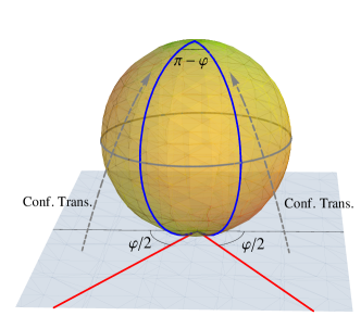
Figure 2: The cusp in the plane $x^{0}=1/2$ is mapped into the spherical wedge under the conformal transformation generated by the vector $(1,0,0)$.

in $\mathcal{N}=4$ SYM, since its value is known at all order in the coupling constant. It was argued in Drukker:2007qr that the exact quantum result is obtained from the ordinary circular Wilson loop computation, with $\lambda$ replaced by

$$\lambda\mapsto\tilde{\lambda}=\lambda\frac{4A_{1}A_{2}}{A^{2}},$$ (45)

where $A_{1}$ and $A_{2}$ are the areas of the two sides of the contour and $A=A_{1}+A_{2}$ is the total area of the two-sphere. Since the DGRT spherical wedge can be related to the BPS configuration of the generalized cusp in $\mathcal{N}=4$ through a special conformal transformation, it is tempting to investigate what is the image of the operator defined in subsect. 3.1 when we map the plane supporting it onto a sphere $S^{2}$.

Our starting point is not the cusp in the plane $(1,2)$, as in subsect. 3.1, but for simplicity one located in the plane $x^{0}=1/2$, i.e.

$$x^{0}=1/2\ \ \ \ \ x^{1}=s\cos\frac{\varphi}{2}\ \ \ \ \ x^{2}=|s|\sin\frac{\varphi}{2}\ \ \ \ -\infty\leq s,\leq\infty.$$ (46)

The plane $x^{0}=1/2$ can be mapped into the usual unit sphere centered in the origin through the special conformal transformation generated by the vector $b^{\mu}=(1,0,0)$

$$y^{0}=\frac{x^{0}-x^{\mu}x_{\mu}}{1-2x^{0}+x^{\mu}x_{\mu}},\ \ \ \ \ y^{1}=\frac{x^{1}}{1-2x^{0}+x^{\mu}x_{\mu}},\ \ \ \ \ y^{2}=\frac{x^{2}}{1-2x^{0}+x^{\mu}x_{\mu}}.$$ (47)

Then the image of the original contour is the wedge illustrated in fig. 2. The new path in terms of $s$ is given by

$$\!\!y^{0}=\frac{\frac{1}{4}-s^{2}}{\frac{1}{4}+s^{2}},\ \ y^{1}=\frac{s\cos\frac{\varphi}{2}}{\frac{1}{4}+s^{2}},\ \ y^{2}=\frac{|s|\sin\frac{\varphi}{2}}{\frac{1}{4}+s^{2}}.$$ (48)

When $s$ ranges from $-\infty$ to $\infty$ we move from the south of the sphere $(-1,0,0)$ to the north pole $(1,0,0)$ [$s=0$] and back to the south pole. The usual parametrization in polar coordinates is recovered by performing the substitution $s=\frac{1}{2}\tan\frac{t}{2}$ in (48)

$$\!\!y^{0}\!=\!\cos t,\ y^{1}\!=\sin t\cos\frac{\varphi}{2},\ y^{2}=|\sin t|\sin\frac{\varphi}{2}$$ (49)

where $t\in[-\pi,\pi]$. The effect of the change of coordinates (47) on the fermionic couplings $\eta_{I}$ and $\bar{\eta}^{I}$ is more interesting and straightforward to determine once we recall the result of a finite special conformal transformation on a spinor field (see e.g. Ho ). Comparing the anti-diagonal term of the matrix (9) in the two different coordinates, we find for instance

$$|\dot{y}|\eta^{\prime}_{I}\bar{\psi}^{\prime I}(y)=|\dot{x}|(1-2(b\cdot x)+b^{2}x^{2})^{-1/2}\eta^{\prime}_{I}(\mathds{1}-b^{\mu}\gamma_{\mu}x^{\alpha}\gamma_{\alpha})\bar{\psi}^{I}(x)=|\dot{x}|\eta_{I}\bar{\psi}^{I}(x),$$ (50)

namely

$$\eta^{\prime}_{I}=\eta_{I}\frac{(\mathds{1}-x^{\alpha}\gamma_{\alpha}b^{\mu}\gamma_{\mu})}{\sqrt{1-2(b\cdot x)+b^{2}x^{2}}}.$$ (51)

In other words, in the case of the spinor couplings, the effect of mapping the cusp into spherical wedge translates into a local rotation defined by the matrix appearing in (51). We have a different rotation on each edge

Edge I:

$(s<0)$

$$R_{I}=\left(\begin{array}[]{cc}\frac{1}{\sqrt{4s^{2}+1}}&\frac{2e^{\frac{i\varphi}{2}}s}{\sqrt{4s^{2}+1}}\\ -\frac{2e^{-\frac{i\varphi}{2}}s}{\sqrt{4s^{2}+1}}&\frac{1}{\sqrt{4s^{2}+1}}\end{array}\right)=\left(\begin{array}[]{cc}\cos\frac{t}{2}&e^{\frac{i\varphi}{2}}\sin\frac{t}{2}\\ -e^{-\frac{i\varphi}{2}}\sin\frac{t}{2}&\cos\frac{t}{2}\end{array}\right)$$ (52a)

Edge II:

$(s>0)$

$$R_{II}=\left(\begin{array}[]{cc}\frac{1}{\sqrt{4s^{2}+1}}&\frac{2e^{-\frac{i\varphi}{2}}s}{\sqrt{4s^{2}+1}}\\ -\frac{2e^{\frac{i\varphi}{2}}s}{\sqrt{4s^{2}+1}}&\frac{1}{\sqrt{4s^{2}+1}}\end{array}\right)=\left(\begin{array}[]{cc}\cos\frac{t}{2}&e^{-\frac{i\varphi}{2}}\sin\frac{t}{2}\\ -e^{\frac{i\varphi}{2}}\sin\frac{t}{2}&\cos\frac{t}{2}\end{array}\right).$$ (52b)

We have expressed the rotation matrices in terms of both the original parameter $s$ and the parameter $t=2\arctan(2s)$. Now the fermionic couplings on the two sides of the wedge are obtained by rotating the old ones by means of the two matrices $R_{I}$ and $R_{II}$

$$\upsilon_{1}^{\alpha}=(\eta_{1}R_{I})^{\alpha}=\mbox{\small$\left(e^{-i\frac{\varphi}{4}}\left(\cos\frac{t}{2}-\sin\frac{t}{2}\right)\ \ e^{i\frac{\varphi}{4}}\left(\cos\frac{t}{2}+\sin\frac{t}{2}\right)\right)$}$$ (53)

$$\upsilon_{2}^{\alpha}=(\eta_{2}R_{II})^{\alpha}=\mbox{\small$\left(e^{i\frac{\varphi}{4}}\left(\cos\frac{t}{2}-\sin\frac{t}{2}\right)\ \ e^{-i\frac{\varphi}{4}}\left(\cos\frac{t}{2}+\sin\frac{t}{2}\right)\right)$}$$ (54)

and obviously $\bar{\upsilon}_{1,2\alpha}=i(\upsilon_{1,2}^{\alpha})^{\dagger}$. The matrices $M$ and $\widehat{M}$ which couple the scalars to the loop are instead unaffected by the special conformal transformation.

Next we consider the effect of the change of variables (47) on the preserved super-charges of subsect. 3.2. The super-conformal Killing spinors $(\bar{\theta}^{IJ},\bar{\vartheta}^{IJ})$ of the cusp are transformed into

$$(\bar{\theta}^{IJ},\bar{\vartheta}^{IJ})\mapsto(\bar{\theta}^{IJ},\bar{\vartheta}^{{}^{\prime}IJ})=(\bar{\theta}^{IJ},\bar{\vartheta}^{IJ}+\bar{\theta}^{IJ}(b^{\mu}\gamma_{\mu}))=(\bar{\theta}^{IJ},\bar{\vartheta}^{IJ}+\bar{\theta}^{IJ}\gamma_{0}).$$ (55)

The loop operator defined by this spherical wedge is preserved by the conformal Killing spinors with a structure given by $\bar{\Theta}^{IJ}=\bar{\theta}^{IJ}(1+y^{\mu}\gamma_{0}\gamma_{\mu})+y^{\mu}\bar{\vartheta}^{IJ}\gamma_{\mu}.$

In doing the conformal transformation we have effectively compactified the contour and we have to understand what happens to the gauge functions at the south pole: continuity of the gauge transformations at north pole is instead inherited by the BPS properties of the open cusp. It is a straightforward exercise to compute the spinor contractions which are relevant in determining the gauge function $g_{1}$ and $\bar{g}_{2}$ at the points $t=-\pi$ and $t=\pi$:

$$\begin{array}[]{llll}\left.g_{1}\right|_{t=-\pi}=4i\sqrt{\frac{2\pi}{k}}(\bar{\tilde{v}}^{L}_{1}C_{L})&&&\left.g_{1}\right|_{t=\pi}=-4i\sqrt{\frac{2\pi}{k}}(\bar{\tilde{v}}^{L}_{2}C_{L})\\ &&&\\ \left.\bar{g}_{2}\right|_{t=-\pi}=4\sqrt{\frac{2\pi}{k}}(\tilde{u}_{1L}\bar{C}^{L})&&&\left.\bar{g}_{2}\right|_{t=\pi}=-4\sqrt{\frac{2\pi}{k}}(\tilde{u}_{2L}\bar{C}^{L})\end{array}$$ (56)

where we used that $\vartheta^{IJ}$ admits the same expansion of the Poincarè supercharges in terms of two vectors $\tilde{u}_{i}$ and $\bar{\tilde{v}}_{i}$. These last two vectors will obey the same constraint of $u_{i}$ and $\bar{v}_{i}$ and in particular for the shared supercharges $\bar{\tilde{v}}^{I}_{1}=\bar{\tilde{v}}^{I}_{2}$ and $\tilde{u}^{I}_{1}=\tilde{u}^{I}_{2}$. We see the gauge functions (56) are anti-periodic and consequently, to have a BPS loop, we have to take the trace to obtain a supersymmetric wedge on $S^{2}$. This is consistent with the result of Drukker:2009hy , our wedge being a non-trivial BPS deformation of the BPS circle. It is interesting that within our construction the antiperiodicity of gauge functions appears as an effect of the conformal mapping, rather that being assumed from the beginning. The presence of such supersymmetric configurations suggests also that it should be possible to construct a general class of BPS loops on $S^{2}$, representing the ABJ analogue of the DGRT loops of ${\cal N}=4$. The explicit construction and the quantum analysis of this new family, as well as of the analogue of Zarembo’s loops in superconformal Chern-Simons theories, will be the subjects of a separate publication CGMS .

4 Quantum results

We shall compute the expectation value of the generalized cusp operator up to the second order in the coupling constant $\left(\frac{2\pi}{\kappa}\right)$. So far there are very few results about the perturbative properties of supersymmetric Wilson loops in ABJ(M) theories and they are all strictly confined to the 1/6 BPS bosonic case Drukker:2008zx ; Chen:2008bp ; Rey:2008bh . We remark that even the matrix model Drukker:2009hy - believed to capture the exact result for the 1/2 BPS circle - has not been verified by explicit Feynman diagrams computations.

The quantum holonomy of the super-connection ${\cal L}$ in a representation ${\cal R}$ of the supergroup $U(N|M)$ is by definition

$$\left\langle\mathcal{W}_{\cal R}\right\rangle=\frac{1}{{\rm dim}_{\cal R}}\int{\cal D}[A,\hat{A},C,\bar{C},\psi,\bar{\psi}]~{}{\rm e}^{-S_{\rm ABJ}}~{}{\rm Tr}_{\cal R}\left[{\rm P}\exp\left(-i\int_{\Gamma}d\tau\,{\cal L}(\tau)\right)\right],$$ (57)

where $S_{ABJ}$ is the Euclidean action for $ABJ(M)$ theories (the part relevant for our computation is spelled out in app. A). In the following $\mathcal{R}$ will be chosen to be the fundamental representation.

In order to evaluate $\left\langle\mathcal{W}_{\cal R}\right\rangle$ we shall first focus our attention on the upper left $N\times N$ block of the super-matrix appearing in (57). For this sub-sector the trace is obviously taken in the fundamental representation ${\bf N}$ of the first gauge group. The result for the lower diagonal block can be then recovered from this analysis by exchanging $N$ with $M$. Our perturbative computation requires to expand the path-exponential in (57) up to the fourth order. The terms in this expansion relevant for the upper block include both bosonic and fermionic monomials:

$$\mathbb{W}_{\mathbf{N}} ={\rm Tr}_{\mathbf{N}}\left[1+i\int_{\Gamma}d\tau_{1}{\cal A}_{1}-\int_{\Gamma}d\tau_{\mbox{\tiny$\displaystyle 1\!\!>\!\!2$}}\Biggl{(}{\cal A}_{1}{\cal A}_{2}-(\eta\bar{\psi})_{1}(\psi\bar{\eta})_{2}\Biggr{)}\right.$$

$$-i\int_{\Gamma}d\tau_{\mbox{\tiny$\displaystyle 1\!\!>\!\!2\!\!>\!\!3$}}\Biggl{(}{\cal A}_{1}{\cal A}_{2}{\cal A}_{3}+\frac{2\pi}{k}[(\eta\bar{\psi})_{1}(\psi\bar{\eta})_{2}{\cal A}_{3}+(\eta\bar{\psi})_{1}\hat{\cal A}_{2}(\psi\bar{\eta})_{3}+{\cal A}_{1}(\eta\bar{\psi})_{2}(\psi\bar{\eta})_{3}]\Biggr{)}$$

$$\left.+\int_{\Gamma}d\tau_{\mbox{\tiny$\displaystyle 1\!\!>\!\!2\!\!>3\!\!>4$}}\left(\left(\frac{2\pi}{\kappa}\right)^{2}(\eta\bar{\psi})_{1}(\psi\bar{\eta})_{2}(\eta\bar{\psi})_{3}(\psi\bar{\eta})_{4}+\mathcal{A}_{1}\mathcal{A}_{2}\mathcal{A}_{3}\mathcal{A}_{4}-\right.\right.$$ (58)

$$-\left(\frac{2\pi}{\kappa}\right)\mathcal{A}_{1}\mathcal{A}_{2}(\eta\bar{\psi})_{3}(\psi\bar{\eta})_{4}-\left(\frac{2\pi}{\kappa}\right)\mathcal{A}_{1}(\eta\bar{\psi})_{2}\hat{\mathcal{A}}_{3}(\psi\bar{\eta})_{4}-\left(\frac{2\pi}{\kappa}\right)(\eta\bar{\psi})_{1}\hat{\mathcal{A}_{2}}\hat{\mathcal{A}_{3}}(\psi\bar{\eta})_{4}-$$

$$\left.\left.-\left(\frac{2\pi}{\kappa}\right)\mathcal{A}_{1}(\eta\bar{\psi})_{2}(\psi\bar{\eta})_{3}\mathcal{A}_{4}-\left(\frac{2\pi}{\kappa}\right)(\eta\bar{\psi})_{1}\hat{\mathcal{A}}_{2}(\psi\bar{\eta})_{3}\mathcal{A}_{4}-\left(\frac{2\pi}{\kappa}\right)(\eta\bar{\psi})_{1}(\psi\bar{\eta})_{2}\mathcal{A}_{3}\mathcal{A}_{4}\right)\right].$$

In (4) we have introduced a shorthand notation for the circuit parameter dependence of the fields, namely ${\cal A}_{i}={\cal A}(x_{i})$ with $x_{i}=x(\tau_{i})$. We have also suppressed the spinor and $SU(4)_{R}$ indices and choosen the parametrization with $|\dot{x}|=1$. The expression above is not symmetric in the exchange of the two gauge groups: the symmetry between them will be recovered when considering also the contribution coming from the lower right $M\times M$ block.

4.1 One-loop analysis

The first non-trivial contributions are proportional to $\left(\frac{2\pi}{\kappa}\right)$ and involve both bosonic and fermionic diagrams. They are listed in fig. 3. Differently from what occurs for the ${\cal N}=4$ generalized cusp, the diagrams which involve only one edge do not vanish when we add them up. The situation is a little more intricate and it is actually convenient to deal with them separately, also in view of the two-loop computation.

The evaluation of the diagrams in fig. 3 obviously encounter UV divergences which originate from the part of the integration region where the propagator endpoints coincide. To tame these divergences we will extensively use dimensional regularization. However regularizing Chern-Simons-matter theories going off-dimensions raises some concerns because of the presence of the anti-symmetric $\epsilon^{\mu\nu\rho}$ tensor. We will follow the DRED scheme, shifting the dimension to $d=3-2\epsilon$ while keeping the Dirac algebra and $\epsilon^{\mu\nu\rho}$ tensor strictly in 3 dimensions. Note that this breaks the conformal invariance introducing a mass scale $\mu^{2\epsilon}$ that keeps the action dimensionless. We will also need an explicit IR regulator $L$, representing the finite length of the two rays forming the cusp: because of the underlying conformal invariance we expect that it could be always scaled away, combining into the $(\mu L)^{2\epsilon}$ to some powers that weights the relevant Feynman integrals.

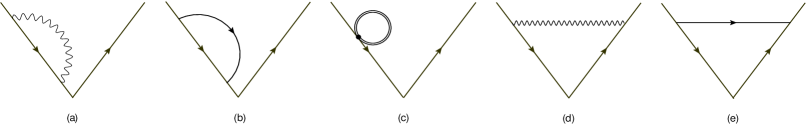
Figure 3: At one-loop order there are only two classes of diagrams: single-edge diagrams [(a), (b) and (c)] and exchange diagrams [(d) and (e)]. The scalar field enters the loop operator only through the composite bilinear $M^{I}_{J}C_{I}\bar{C}^{J}$, and its conjugate $\widehat{M}^{I}_{J}\bar{C}^{J}C_{I}$, hence the exchange of a single scalar is not permitted.

We start by considering the bosonic diagrams: the scalar tadpole of fig. 3.(c), that originates from the first term in the expansion (4), vanishes in our regularization procedure and we can safely forget its existence in the following. The bosonic contributions in fig. 3.(a) and 3.(d) stems from the term with two gauge fields in (4) and they can be cast into a single path-ordered integral,

$$\mathfrak{B}^{(1)}={\rm i}N^{2}\left(\frac{\mu^{2\epsilon}}{\kappa}\right)\frac{\Gamma(\frac{3}{2}-\epsilon)}{\pi^{\frac{1}{2}-\epsilon}}\,\int_{\Gamma}d\tau_{\mbox{\tiny$\displaystyle 1\!\!>\!\!2$}}\,\frac{\epsilon_{\mu\nu\rho}\dot{x}_{1}^{\mu}\dot{x}_{2}^{\nu}(\dot{x}_{1}-\dot{x}_{2})^{\rho}}{|x_{1}-x_{2}|^{3-2\epsilon}}=0,$$ (59)

whose integrand vanishes for any planar loop due to the antisymmetry of the $\epsilon-$tensor. We have used here the explicit form of the Chern-Simons propagator in position space, presented in App. B. We remark that the same result would have been obtained if we have used 1/6 BPS lines, in spite of the different structure of the mass-matrix $M^{I}_{J}$.

Next we discuss the fermionic diagrams in fig. 3. They represent the true novelty of the present calculation and originate from taking the vacuum expectation value of the fermionic bilinear in the first line of (4)

$$\mathfrak{F}^{(1)}=\left(\frac{2\pi}{\kappa}\right)\mu^{2\epsilon}\int_{\tau_{2}<\tau_{1}}\!\!\!\!\!d\tau_{1}d\tau_{2}~{}\langle\mathrm{Tr}_{\bf N}\left[(\eta\bar{\psi})_{1}(\psi\bar{\eta})_{2}\right]\rangle=\left(\frac{2\pi}{\kappa}\right)\mu^{2\epsilon}({\cal F}_{b}+{\cal F}_{e}),$$ (60)

where we have denoted with ${\cal F}_{b}$ and ${\cal F}_{e}$ the contributions corresponding to the graphs 3.(b) and 3.(e) respectively. At the lowest order, the vacuum expectation value in (60) is simply obtained by contracting the fermion propagator (B.147) with the spinors $\eta$ and $\bar{\eta}$. We find

$$\langle\mathrm{Tr}_{\bf N}\left[(\eta\bar{\psi})_{1}(\psi\bar{\eta})_{2}\right]\rangle=iMN\frac{\Gamma(1/2-\epsilon)}{4\pi^{3/2-\epsilon}}\eta_{L1}\gamma^{\mu}\bar{\eta}_{2}^{L}\partial_{x^{\mu}_{1}}\left(\frac{1}{(x_{12}^{2})^{1/2-\epsilon}}\right),$$ (61)

where $x_{ij}=x_{i}-x_{j}$. The fermion bilinear $\eta_{L1}\gamma_{\mu}\bar{\eta}_{2}^{L}$ can be readily evaluated for a general contour (and for general parametrization), thanks to the factorized form (10) of the spinor couplings and to the identity (B.163). We have

$$(\eta_{L1}\gamma^{\mu}\bar{\eta}_{2}^{L})=-2\frac{(n_{1}\cdot\bar{n}_{2})}{(\eta_{2}\bar{\eta}_{1})}\left[\frac{\dot{x_{1}}^{\mu}}{|\dot{x}_{1}|}+\frac{\dot{x_{2}}^{\mu}}{|\dot{x}_{2}|}+\frac{1}{2}\frac{\dot{x_{1}}^{\lambda}}{|\dot{x}_{1}|}\frac{\dot{x_{2}}^{\nu}}{|\dot{x}_{2}|}{\rm i}\epsilon^{\lambda\mu\nu}\right].$$ (62)

Since $\dot{x}_{1}$, $\dot{x}_{2}$ and $x_{12}=-x_{21}$ lay on the same plane, we can drop the wedge product in (62) and we obtain the following result

$$\langle\mathrm{Tr}_{\bf N}\left[(\eta\bar{\psi})_{1}(\psi\bar{\eta})_{2}\right]\rangle=-\frac{iMN\Gamma(1/2-\epsilon)}{2\pi^{3/2-\epsilon}(\eta_{2}\bar{\eta}_{1})}(n_{L1}\bar{n}^{L}_{2})\left[\frac{\dot{x}_{1}^{\mu}}{|\dot{x_{1}}|}+\frac{\dot{x_{2}}^{\mu}}{|\dot{x}_{2}|}\right]\partial_{x_{1}^{\mu}}\left(\frac{1}{(x_{12}^{2})^{1/2-\epsilon}}\right),$$ (63)

which holds for any planar circuit. Let us specialize (60) to the diagram of 3(e): within our parametrization of the circuit, we can rearrange the effective propagator exchanged through the rays as the difference of two total derivatives

$$\left[\frac{\dot{x}_{1}^{\mu}}{|\dot{x_{1}}|}+\frac{\dot{x_{2}}^{\mu}}{|\dot{x}_{2}|}\right]\partial_{x_{1}^{\mu}}\left(\frac{1}{(x_{12}^{2})^{1/2-\epsilon}}\right)=\left(\frac{d}{d\tau_{1}}-\frac{d}{d\tau_{2}}\right)\frac{1}{(\tau_{1}^{2}+\tau_{2}^{2}-2\tau_{1}\tau_{2}\cos\varphi)^{1/2-\epsilon}}.$$ (64)

The integration over the two edges can be done in a rather trivial way

$$\begin{split}&\int_{0}^{L}d\tau_{1}\int_{-L}^{0}d\tau_{2}\left(\frac{d}{d\tau_{1}}-\frac{d}{d\tau_{2}}\right)\frac{1}{(\tau_{1}^{2}+\tau_{2}^{2}-2\tau_{1}\tau_{2}\cos\varphi)^{1/2-\epsilon}}=\\ &=-\frac{L^{2\epsilon}}{\epsilon}+2L^{2\epsilon}\int_{0}^{1}d\tau\frac{1}{(\tau^{2}+2\tau\cos\varphi+1)^{1/2-\epsilon}}.\end{split}$$ (65)

The remaining integral in (65) is finite as $\epsilon\to 0$ and it can be evaluated in terms of hypergeometric functions. However its exact value for arbitrary $\epsilon$ will not be relevant for us and we shall only give its expansion around $\epsilon=0$ at the lowest order

$$\int_{0}^{1}d\tau\frac{1}{(\tau^{2}+2\tau\cos\varphi+1)^{1/2-\epsilon}}=\log\left(\sec\left(\frac{\varphi}{2}\right)+1\right)+O(\epsilon).$$ (66)

We end up with

$${\cal F}_{e}=\frac{iMN\Gamma(1/2-\epsilon)}{2\pi^{3/2-\epsilon}(\nu_{1}\bar{\nu}_{2})}(n_{L2}\bar{n}^{L}_{1})L^{2\epsilon}\left[\frac{1}{\epsilon}-2\log\left(\sec\left(\frac{\varphi}{2}\right)+1\right)\right]$$ (67)

and since $(n_{L2}\bar{n}^{L}_{1})=\cos\frac{\theta}{2}$ and $(\nu_{1}\bar{\nu}_{2})=2i\cos\frac{\varphi}{2}$ we get

$${\cal F}_{e}=MN\left(\frac{\Gamma(1/2-\epsilon)}{4\pi^{3/2-\epsilon}}\right)\frac{\cos\frac{\theta}{2}}{\cos\frac{\varphi}{2}}L^{2\epsilon}\left[\frac{1}{\epsilon}-2\log\left(\sec\left(\frac{\varphi}{2}\right)+1\right)\right].$$ (68)

Next we must consider the case where the fermionic propagator connects two points on the same edge of the cusp, i.e. the diagrams (b) in fig. 3. We have two mirror graphs: one for each edge. The result of the first one is provided by

$$-\frac{MN\Gamma(1/2-\epsilon)}{4\pi^{3/2-\epsilon}}\int_{-L}^{0}\!\!\!d\tau_{1}\int_{-L}^{\tau_{1}}\!\!d\tau_{2}\left(\frac{d}{d\tau_{1}}-\frac{d}{d\tau_{2}}\right)\frac{1}{(\tau_{1}-\tau_{2})^{1-2\epsilon}}=-\frac{MN\Gamma(1/2-\epsilon)}{4\pi^{3/2-\epsilon}}\frac{L^{2\epsilon}}{\epsilon},$$ (69)

while the contribution of the second one simply doubles (69) and it yields

$${\cal F}_{b}=-2\frac{MN\Gamma(1/2-\epsilon)}{4\pi^{3/2-\epsilon}}\frac{L^{2\epsilon}}{\epsilon}.$$ (70)

Therefore the complete one loop result for the upper left block can be written as

$$\mathfrak{F}^{(1)}=\left(\frac{2\pi}{\kappa}\right)MN\left(\frac{\Gamma(1/2-\epsilon)}{4\pi^{3/2-\epsilon}}\right)(\mu L)^{2\epsilon}\left[\frac{1}{\epsilon}\left(\frac{\cos\frac{\theta}{2}}{\cos\frac{\varphi}{2}}-2\right)-2\frac{\cos\frac{\theta}{2}}{\cos\frac{\varphi}{2}}\log\left(\sec\left(\frac{\varphi}{2}\right)+1\right)\right].$$ (71)

This result may appear surprising at a first sight: while we could have expected the divergence from the cusp diagram (e), we have also a non-trivial contribution from the propagators living on a single edge (b). In ${\cal N}=4$ SYM theory the analogous contributions, coming from the combined gauge-scalar propagator, are identically zero in Feynman gauge, and their potential divergence never enters into the game. Moreover in the limit $\varphi=\theta=0$ a non-vanishing and divergent result persists, contradicting the naive expectation that the BPS infinite line is trivial. To understand the result (71) and to extract from it the truly gauge-invariant cusp divergence, we have to recall some basics about the renormalization of (cusped) Wilson loops in gauge theories and to adapt the general procedure to our somehow exotic operators: this will be done in the next section, after having completed the two-loop computation.

The full one-loop expression is recovered by considering also the part coming from the lower $M\times M$ block of the super-holonomy: it turns out to be the same, because of the symmetry between $N$ and $M$ at this order. The trace is simply obtained by adding this second contribution.

5 Two-loop analysis

We shall compute here the second order contribution to the expectation value of the cusped Wilson loop: we separate the computations of purely bosonic diagrams from fermionic ones, to appreciate technical and conceptual differences.

5.1 Bosonic diagrams

When expanding the Wilson loop operator at the second order in the coupling constant, we encounter the four families of merely bosonic contributions depicted in fig. 4. We consider first the diagrams containing the one-loop corrected gluon propagators (fig. 4.(a)). As we did in the one-loop analysis, we shall focus our attention on the upper diagonal block of the super-matrix, i.e. on the $U(N)$ sector. With the help of (B.149), where the one-loop propagator is presented, we can immediately write

$$\begin{split}\left[\ref{BosonicDiagrams}.(a)\right]_{\rm up}\!=\!-MN^{2}\left(\frac{2\pi}{\kappa}\right)^{2}\frac{\Gamma^{2}\left(\frac{1}{2}-\epsilon\right)}{4\pi^{3-2\epsilon}}\int_{\Gamma}d\tau_{\mbox{\tiny$\displaystyle 1\!\!>\!\!2$}}\!\left[\frac{(\dot{x}_{1}\cdot\dot{x}_{2})}{((x-y)^{2})^{{1}-2\epsilon}}-\partial_{\tau_{1}}\partial_{\tau_{2}}\!\frac{((x_{1}-x_{2})^{2})^{\epsilon}}{4\epsilon(1+2\epsilon)}\right]\!.\end{split}$$ (72)

A similar structure is obtained when considering the correlator of two scalar composite operators $M_{I}^{\ J}C_{J}\bar{C}^{I}$ in the diagram 4.(b):

$$\begin{split}\left[\ref{BosonicDiagrams}.(b)\right]_{\rm up}=MN^{2}\left(\frac{2\pi}{\kappa}\right)^{2}\frac{\Gamma^{2}\left(\frac{1}{2}-\epsilon\right)}{16\pi^{3-2\epsilon}}\int_{\Gamma}d\tau_{\mbox{\tiny$\displaystyle 1\!\!>\!\!2$}}\ \frac{|\dot{x}_{1}||\dot{x}_{2}|{\rm Tr}(M_{1}M_{2})}{((x-y)^{2})^{{1}-2\epsilon}}.\end{split}$$ (73)

The integrals (72) and (73) can be naturally combined together to give

$$\!-MN^{2}\left(\frac{2\pi}{\kappa}\right)^{\!\!2}\!\frac{\Gamma^{2}\!\left(\frac{1}{2}-\epsilon\right)}{4\pi^{3-2\epsilon}}\!\int_{\Gamma}\!d\tau_{\mbox{\tiny$\displaystyle 1\!\!>\!\!2$}}\!\left[\frac{(\dot{x}_{1}\!\cdot\!\dot{x}_{2})-\frac{1}{4}|\dot{x}_{1}||\dot{x}_{2}|{\rm Tr}(M_{1}M_{2})}{((x-y)^{2})^{{1}-2\epsilon}}-\partial_{\tau_{1}}\partial_{\tau_{2}}\frac{((x_{1}-x_{2})^{2})^{\epsilon}}{4\epsilon(1+2\epsilon)}\right]\!\!.$$ (74)

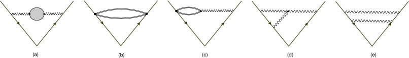
Figure 4: Two loops bosonic diagrams: (a) One-loop corrected gauge propagators; (b) Correlators of two composite scalar operators; (c) Correlators gauge field composite scalar operator; (d) Chern-Simons vertex diagrams; (e) Gluon double exchange diagrams.

The result (74) deserves some comments. The last term in (74) is a total derivative and it would correspond to a gauge transformation -albeit a singular one. In dimensional regularization it yields a $(\theta,\varphi)$ independent pole in $\epsilon$ plus finite terms, thus its contribution to the divergent part of the cusp becomes ineffective when we impose the renormalization condition discussed in subsec. 4.1. The other contribution in (74), as firstly noted in Drukker:2008zx , possesses an unforeseen four-dimensional structure. When the two endpoints lie on the same edge it is proportional to the the tree-level effective propagator in $\mathcal{N}=4$ since $\mathrm{Tr}(M_{1}M_{2})=4$ and thus it vanishes. If they lie instead on opposite edges we get the following result

$$\mathfrak{B}^{(2)}=-MN^{2}\left(\frac{2\pi}{\kappa}\right)^{\!\!2}\!\frac{\Gamma^{2}\!\left(\frac{1}{2}-\epsilon\right)}{4\pi^{3-2\epsilon}}\left(\cos\varphi-\cos^{2}\frac{\theta}{2}\right)\!\int_{0}^{L}\!\!\!d\tau_{1}\int_{-L}^{0}\!\!\!d\tau_{2}\frac{1}{((x-y)^{2})^{{1}-2\epsilon}},$$ (75)

where the integral governing the divergence is the same of the four dimensional case when we replace $2\epsilon$ with $\epsilon$.

Next we examine the graphs 4.(c), 4.(d) and 4.(e). The last one is identically zero for the same reasons of the one-loop single exchange 3.(a). The diagram 4.(c) for the case of planar loop was discussed in Drukker:2008zx where it was found to vanish. The same fate is shared by 4.(d) as pointed out in Henn:2010ps . The only contribution originating from the bosonic diagrams is therefore provided by (75).

5.2 Fermionic diagrams

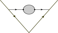
Figure 5: One-loop corrected fermions propagators

The simplest fermionic diagram appearing at the second order in perturbation theory consists of the exchange of the one-loop corrected fermion propagator depicted in fig 5.

The one-loop two-point function for the spinor fields is briefly discussed in app. B. Remarkably it again displays the four dimensional behaviour already encountered in the bosonic case. Its form, in the DRED scheme, is

$$\left\langle(\psi_{I})_{\hat{i}}^{\ j}(x)(\bar{\psi}^{J})_{k}^{\ \hat{l}}(y)\right\rangle^{1~{}\rm\ell oop}_{0}=-i\left(\frac{2\pi}{\kappa}\right)\delta_{\hat{i}}^{\\ \hat{l}}\delta^{j}_{k}(N-M)\frac{\Gamma^{2}\left(\frac{1}{2}-\epsilon\right)}{16\pi^{3-2\epsilon}}\frac{1}{((x-y)^{2})^{1-2\epsilon}}.$$ (76)

The contribution to the upper block of the Wilson loop takes the following form

$$\begin{split}\left(\frac{2\pi\mu^{2\epsilon}}{\kappa}\right)^{2}iMN(N-M)\frac{\Gamma^{2}\left(\frac{1}{2}-\epsilon\right)}{16\pi^{3-2\epsilon}}\int_{\Gamma}d\tau_{\mbox{\tiny$\displaystyle 1\!\!>\!\!2$}}\frac{(\eta_{I1}\bar{\eta}^{I}_{2})}{((x_{1}-x_{2})^{2})^{1-2\epsilon}}\end{split}$$ (77)

5.2.1 Double Exchanges

We come now to discuss a more subtle group of diagrams, namely those involving two $\langle\psi\bar{\psi}\rangle$ propagators. They arise when we evaluate the contribution of the fermionic quadrilinear in (4). At this order its expansion yields only two sets of non-vanishing Wick-contractions, weighted by different group factor, and thus we arrive at the following integral

$$\begin{split}&-4\left(\frac{2\pi\mu^{2\epsilon}}{\kappa}\right)^{\!\!2}\!\int_{\Gamma}\!\!d\tau_{\mbox{\tiny$\displaystyle 1\!\!>\!\!2\!\!>\!\!3\!\!>\!\!4$}}[M^{2}N\underset{(A1)}{S(x_{2}-x_{1})S(x_{4}-x_{3})}-N^{2}M\underset{(B1)}{S(x_{2}-x_{3})S(x_{4}-x_{1})}].\end{split}$$ (78)

Here the function $S(x_{i}-x_{j})$ is proportional to the two-point fermion correlator already encountered in (61) and it can be conveniently written as

$$S(x_{i}-x_{j})=\frac{(n_{i}\cdot n_{j})}{(\eta_{j}\bar{\eta}_{i})}(\partial_{\tau_{i}}-\partial_{\tau_{j}})D(x_{i}-x_{j}),$$ (79)

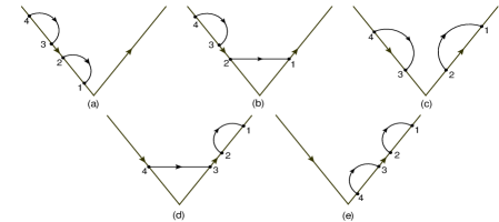
Figure 6: First group of double-exchange diagrams

where $D(x_{i}-x_{j})$ is the free scalar propagator defined in (B.146) while the couple of vectors $(n_{iI},\bar{n}_{i}^{I})$ and of spinors $(\eta_{Ii},\bar{\eta}_{i}^{I})$ are defined in sec. 3.1. We shall consider the two contributions in (78) separately. In order to evaluate the term (A1) we have to split the region of integration in five sectors that correspond to the five different Feynman diagrams depicted in fig. 6. Luckily we do not have to compute all of them. In fact graphs, which are related by a reflection with respect to the axis bisecting the cusp, yield the same result. In other words, the following equalities hold among the diagrams of fig.6: 6.(a)=6.(e) and 6.(b)=6.(d). Moreover the graph 6.(c) is simply the square of 3.(b).

To begin with, let us evaluate the contribution 6.(a). It is given by the following integral

$$[\ref{DoubleExc1class}.(a)]_{\rm up}\!=\! \left(\frac{2\pi}{\kappa}\right)^{\!\!2}\!\!M^{2}\!N\frac{\Gamma^{2}\left(\frac{3}{2}-\epsilon\right)}{\pi^{{3}-2\epsilon}}\mu^{4\epsilon}\!\!\int_{-L}^{0}\!\!\!\!\!d\tau_{1}\int_{-L}^{\tau_{1}}\!\!\!\!\!d\tau_{2}\int_{-L}^{\tau_{2}}\!\!\!\!\!d\tau_{3}\int_{-L}^{\tau_{3}}\!\!\!\!\!d\tau_{4}~{}(\tau_{1}-\tau_{2})^{2\epsilon-2}(\tau_{3}-\tau_{4})^{2\epsilon-2}\!\!=$$

$$= \left(\frac{2\pi}{\kappa}\right)^{\!\!2}\!\!M^{2}\!N\frac{\Gamma^{2}\left(\frac{1}{2}-\epsilon\right)}{16\pi^{3-2\epsilon}}\frac{\sqrt{\pi}}{2^{4\epsilon}}\frac{\Gamma(2\epsilon+1)}{\Gamma(2\epsilon+\frac{1}{2})}\frac{(\mu L)^{4\epsilon}}{\epsilon^{2}}.$$ (80)

The diagram 6.(b) instead leads to a different computation

$$\begin{split}\!\!\!\![\ref{DoubleExc1class}.(b)]_{\rm up}\!=\!-\!\left(\frac{2\pi}{\kappa}\right)^{\!\!2}\!\!M^{2}N\frac{\Gamma^{2}\left(\frac{1}{2}-\epsilon\right)}{16\pi^{{3}-2\epsilon}}\frac{\mu^{4\epsilon}}{\epsilon}\frac{\cos\frac{\theta}{2}}{\cos\frac{\varphi}{2}}\int_{0}^{L}\!\!\!\!\!d\tau_{1}\!\!\int_{-L}^{0}\!\!\!\!\!d\tau_{2}(L+\tau_{2})^{2\epsilon}(\partial_{\tau_{2}}\!-\partial_{\tau_{1}})H(\tau_{1},\tau_{2}),\end{split}$$ (81)

where $H(\tau_{1},\tau_{2})=(\tau_{1}^{2}+\tau_{2}^{2}-2\tau_{1}\tau_{2}\cos\varphi)^{-\frac{1}{2}+\epsilon}$. We have performed the two trivial integrations over $\tau_{3}$ and $\tau_{4}$ since they involve a propagator whose endpoints belongs to the same edge. To extract the result we are interested in, we do not need the exact value of the remaining integral, but only its $\epsilon-$expansion up to finite terms discussed in app. C. We get

$$[\ref{DoubleExc1class}.(b)]_{\rm up}\!=\!-\left(\frac{2\pi}{\kappa}\right)^{\!\!2}M^{2}N\frac{\cos\frac{\theta}{2}}{\cos\frac{\varphi}{2}}\frac{\Gamma^{2}(\frac{1}{2}-\epsilon)}{16\pi^{3-2\epsilon}}(L\mu)^{4\epsilon}\left[\frac{1}{\epsilon^{2}}-\frac{2}{\epsilon}\log\left(1+\sec\frac{\varphi}{2}\right)+O(1)\right].$$ (82)

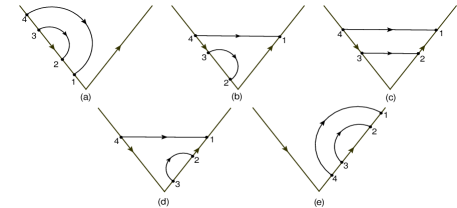
Figure 7: Second group of double-exchange diagrams

The next step is to consider the term (B1) in (78): again we have to separate the region of integration in five sub-sectors and this yields the diagrams in fig. 7. However the same reflection symmetry considered in the case of the term (A1) implies that we have just to compute 7.(a), 7.(b) and 7.(c). The first one can be easily computed in closed form and it gives

$$[\ref{DoubleExc2class}.(a)]_{\rm up}=\left(\frac{2\pi}{\kappa}\right)^{\!\!2}\!\!M\!N^{\!2}\frac{\Gamma\left(\frac{1}{2}-\epsilon\right)^{2}}{16\pi^{3-2\epsilon}}\frac{(2\epsilon-1)}{2(4\epsilon-1)}\frac{(\mu L)^{4\epsilon}}{\epsilon^{2}}.$$ (83)

Concerning the second diagram, we can trivially perform the integration over $\tau_{2}$ and $\tau_{3}$, obtaining

$$\begin{split}[\ref{DoubleExc2class}.(b)]_{\rm up}=-\left(\frac{2\pi}{\kappa}\right)^{\!\!2}\!\!N^{2}M\frac{\Gamma^{2}(\frac{1}{2}-\epsilon)}{16\pi^{3-2\epsilon}}\frac{\cos\frac{\theta}{2}}{\cos\frac{\varphi}{2}}\frac{\mu^{4\epsilon}}{\epsilon}\!\int_{0}^{L}\!\!\!\!d\tau_{1}\int_{-L}^{0}\!\!\!\!d\tau_{4}~{}{(-\tau_{4})^{2\epsilon}}(\partial_{\tau_{4}}-\partial_{\tau_{1}})H(\tau_{1},\tau_{4}).\end{split}$$ (84)

With the help of the results of app. C, we can then write the following $\epsilon-$expansion

$$[\ref{DoubleExc2class}.(b)]_{\rm up}=-\left(\frac{2\pi}{\kappa}\right)^{\!\!2}\!\!N^{2}M\frac{\Gamma^{2}(\frac{1}{2}-\epsilon)}{16\pi^{3-2\epsilon}}\frac{\cos\frac{\theta}{2}}{\cos\frac{\varphi}{2}}{(L\mu)^{4\epsilon}}\left[\frac{1}{2\epsilon^{2}}+\frac{1}{\epsilon}\log\left(\frac{1}{4}\cos\frac{\varphi}{2}\sec^{4}\frac{\varphi}{4}\right)+O(1)\right].$$ (85)

For the graph 7.(c) we shall adopt a different procedure since both propagators connect different edges. First we rearrange its integral expression as follows

$$\begin{split}[\ref{DoubleExc2class}.(c)]_{\rm up}=&-2\left(\frac{2\pi}{\kappa}\right)^{\!\!2}\!N^{2}M\left(\mu^{2\epsilon}\int_{0}^{L}\!\!\!\!\!\!d\tau_{1}\int_{-L}^{0}\!\!\!\!\!\!d\tau_{4}S(x_{4}-x_{1})\right)^{2}-\\ &\ \ \ \ \ \ -4\left(\frac{2\pi}{\kappa}\right)^{\!\!2}\!MN^{2}\mu^{4\epsilon}\int_{0}^{L}\!\!\!\!\!d\tau_{1}\int_{0}^{\tau_{1}}\!\!\!\!\!d\tau_{2}\int_{-L}^{0}\!\!\!\!\!d\tau_{3}\int_{-L}^{\tau_{3}}\!\!\!\!\!d\tau_{4}~{}S(x_{2}-x_{4})S(x_{3}-x_{1}),\end{split}$$ (86)

where we have separated the “abelian” and “non-abelian” part of the diagram. The former is given by the first term, which is proportional to the square of 3.(e), while the latter is identified with the second term in (86). This decomposition also has advantage that the leading divergence $1/\epsilon^{2}$ is only present in the first term.

With the help of the results of app. C, we obtain the following $\epsilon-$expansion for this diagram

$$\begin{split}[\ref{DoubleExc2class}.(c)]_{\rm up}=&\frac{1}{2}\left(\frac{2\pi}{\kappa}\right)^{\!\!2}N^{2}M\frac{\Gamma^{2}(\frac{1}{2}-\epsilon)}{16\pi^{3-2\epsilon}}(L\mu)^{4\epsilon}\left[\frac{\cos\frac{\theta}{2}}{\cos\frac{\varphi}{2}}\left(\frac{1}{\epsilon}-2\log\left(1+\sec\frac{\varphi}{2}\right)\right)\right]^{2}-\\ &\ \ \ \ \ \ -\left(\frac{2\pi}{\kappa}\right)^{\!\!2}N^{2}M\left(\frac{\cos\frac{\theta}{2}}{\cos\frac{\varphi}{2}}\right)^{2}\frac{\Gamma^{2}(\frac{1}{2}-\epsilon)}{16\pi^{3-2\epsilon}}\frac{(L\mu)^{4\epsilon}}{\epsilon}\cos^{2}\frac{\varphi}{2}\frac{\varphi}{\sin\varphi}+O(1).\end{split}$$ (87)

5.2.2 Vertex Diagrams

The final group of fermionic diagrams, which are relevant for our calculation, arises when we expand in perturbation theory the term

$$-\frac{2\pi i}{\kappa}\int_{\Gamma}d\tau_{\mbox{\tiny$\displaystyle 1\!\!>\!\!2\!\!>\!\!3$}}\left\langle(\underset{(\mathrm{{\bf A}_{2}})}{\eta\bar{\psi})_{1}(\psi\bar{\eta})_{2}{\cal A}_{3}}+\underset{(\mathrm{{\bf B}_{2}})}{{\cal A}_{1}(\eta\bar{\psi})_{2}(\psi\bar{\eta})_{3}}+\underset{(\mathrm{{\bf C}_{2}})}{(\eta\bar{\psi})_{1}\hat{\cal A}_{2}(\psi\bar{\eta})_{3}}\right\rangle,$$ (88)

appearing in the upper block (4). At this order the expectation value in (88) is evaluated by just considering the Wick-contractions of the monomials $({\rm{\bf A}_{2}})$, $({\rm\mathrm{{\bf B}_{2}}})$ and $({\rm\mathrm{{\bf C}_{2}}})$ with the tree-level gauge-fermion vertices present in the Lagrangian (A). Then the three different contributions can be rewritten as follows

$$\!\!\!\!\!(\mathrm{{\bf A}_{2}})= -\left(\frac{2\pi}{\kappa}\right)^{2}N^{2}M~{}\int_{\Gamma}d\tau_{\mbox{\tiny$\displaystyle 1\!\!>\!\!2\!\!>\!\!3$}}~{}\eta_{1L}\gamma_{\nu}\gamma^{\mu}\gamma_{\lambda}\bar{\eta}_{2}^{L}\epsilon_{\mu\rho\sigma}\dot{x}_{3}^{\rho}~{}\Gamma^{\nu\lambda\sigma}(x_{1},x_{2},x_{3}),$$ (89a)

$$\!\!\!\!\!(\mathrm{\mathrm{{\bf B}_{2}}})= -\left(\frac{2\pi}{\kappa}\right)^{2}N^{2}M~{}\int_{\Gamma}d\tau_{\mbox{\tiny$\displaystyle 1\!\!>\!\!2\!\!>\!\!3$}}~{}\eta_{2L}\gamma_{\lambda}\gamma^{\mu}\gamma_{\nu}\bar{\eta}^{L}_{3}\epsilon_{\mu\rho\sigma}\dot{x}_{1}^{\rho}~{}\Gamma^{\sigma\lambda\nu}(x_{1},x_{2},x_{3}),$$ (89b)

$$\!\!\!\!\!(\mathrm{\mathrm{{\bf C}_{2}}})= -\left(\frac{2\pi}{\kappa}\right)^{2}NM^{2}\int_{\Gamma}d\tau_{\mbox{\tiny$\displaystyle 1\!\!>\!\!2\!\!>\!\!3$}}~{}\eta_{1L}\gamma_{\lambda}\gamma^{\mu}\gamma_{\nu}\bar{\eta}_{3}^{\ L}\epsilon_{\mu\rho\sigma}\dot{x}_{2}^{\rho}~{}\Gamma^{\lambda\sigma\nu}(x_{1},x_{2},x_{3}),$$ (89c)

where $\Gamma^{\lambda\mu\nu}(x_{1},x_{2},x_{3})$ is a short-hand notation for the three-point function in position space, defined by the integral

$$\begin{split}\Gamma^{\lambda\mu\nu}(x_{1},x_{2},x_{2})=&\left(\frac{\Gamma(\frac{1}{2}-\epsilon)}{4\pi^{3/2-\epsilon}}\right)^{3}\partial_{x_{1}^{\lambda}}\partial_{x_{2}^{\mu}}\partial_{x_{3}^{\nu}}\int\frac{d^{3-2\epsilon}w}{(x_{1w}^{2})^{1/2-\epsilon}(x_{2w}^{2})^{1/2-\epsilon}(x_{3w}^{2})^{1/2-\epsilon}}.\end{split}$$ (90)

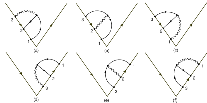
Figure 8: Vertex diagrams where the fermion propagators are attached to the same edge of the gluon propagator.

Diagrammatically the three contributions (89) will lead to graphs which differ for the position of the gauge field along the contour: $(\mathrm{{\bf A}_{2}})$ and $(\mathrm{{\bf B}_{2}})$ only yield diagrams where the gluon is respectively the first or the last field we encounter when $\tau$ runs from $-L$ to $L$; $(\mathrm{{\bf C}_{2}})$ instead corresponds to diagrams where the gauge field is always located between the two fermionic lines. For instance, 8.(a) and 8.(d) originate from $(\mathrm{{\bf A}_{2}})$, 8.(b) and 8.(e) from $(\mathrm{{\bf C}_{2}})$ and 8.(c) and 8.(f) from $(\mathrm{{\bf B}_{2}})$.

If we now expand the spinor bilinears in (89) in terms of the circuit tangent vectors $\dot{x}_{i}$ and of the scalar contraction $(\eta_{i}\bar{\eta}_{j})$, the three contributions $(\mathrm{{\bf A}_{2}})$, $(\mathrm{{\bf B}_{2}})$ and $(\mathrm{{\bf C}_{2}})$ can be rewritten as follows

$$(\mathrm{{\bf A}_{2}})= -N^{2}M\left(\frac{2\pi}{\kappa}\right)^{2}i(n_{1}\cdot n_{2})\oint_{\tau_{1}>\tau_{2}>\tau_{3}}\biggl{[}\frac{2}{(\eta_{2}\bar{\eta}_{1})}\biggl{(}((\dot{x}_{2}\cdot\dot{x}_{3})\dot{x}_{1\nu}-(\dot{x}_{1}\cdot\dot{x}_{3})\dot{x}_{2\nu})[\Gamma^{\nu\tau\tau}+$$

$$\phantom{\Biggl{[}}+\Gamma^{\tau\nu\tau}-\Gamma^{\tau\tau\nu}]+\dot{x}_{1\sigma}\dot{x}_{2\nu}\dot{x}_{3\lambda}\Gamma^{\nu\lambda\sigma}-\dot{x}_{1\nu}\dot{x}_{2\sigma}\dot{x}_{3\lambda}\Gamma^{\nu\lambda\sigma}+\dot{x}_{1\sigma}\dot{x}_{2\lambda}\dot{x}_{3\nu}\Gamma^{\nu\lambda\sigma}-$$

$$-\dot{x}_{1\lambda}\dot{x}_{2\sigma}\dot{x}_{3\nu}\Gamma^{\nu\lambda\sigma}\biggr{)}+{(\eta_{1}\bar{\eta}_{2})\dot{x}_{3\lambda}(\Gamma^{\tau\lambda\tau}-\Gamma^{\lambda\tau\tau})}\Biggr{]},$$ (91a)

$$(\mathrm{{\bf B}_{2}})= -N^{2}M\left(\frac{2\pi}{\kappa}\right)^{2}i(n_{3}\cdot n_{2})\oint_{\tau_{1}>\tau_{2}>\tau_{3}}~{}\Biggl{[}\frac{2}{(\eta_{3}\bar{\eta}_{2})}\biggl{(}[(\dot{x}_{1}\cdot\dot{x}_{3})\dot{x}_{2\nu}-(\dot{x}_{2}\cdot\dot{x}_{1})x_{3\nu}][\Gamma^{\tau\tau\nu}+$$

$$\phantom{\Biggl{[}}+\Gamma^{\tau\nu\tau}-\Gamma^{\nu\tau\tau}]+\dot{x}_{1\lambda}\dot{x}_{2\nu}\dot{x}_{3\sigma}\Gamma^{\nu\lambda\sigma}-\dot{x}_{1\lambda}\dot{x}_{2\sigma}\dot{x}_{3\nu}\Gamma^{\nu\lambda\sigma}+\dot{x}_{1\sigma}\dot{x}_{2\nu}\dot{x}_{3\lambda}\Gamma^{\nu\lambda\sigma}-$$

$$-\dot{x}_{1\sigma}\dot{x}_{2\lambda}\dot{x}_{3\nu}\Gamma^{\nu\lambda\sigma}\biggr{)}+{(\eta_{2}\bar{\eta}_{3})\dot{x}_{1\nu}(\Gamma^{\tau\tau\nu}-\Gamma^{\tau\nu\tau})}\Biggr{]},$$ (91b)

$$(\mathrm{{\bf C}_{2}})= -NM^{2}\left(\frac{2\pi}{\kappa}\right)^{2}i(n_{1}\cdot n_{3})\oint_{\tau_{1}>\tau_{2}>\tau_{3}}\Biggl{[}\frac{2}{(\eta_{3}\bar{\eta}_{1})}\biggl{(}((\dot{x}_{2}\cdot\dot{x}_{3})\dot{x}_{1\nu}-(\dot{x}_{1}\cdot\dot{x}_{2})\dot{x}_{3\nu})[\Gamma^{\tau\tau\nu}+$$

$$\phantom{\Biggl{[}}+\Gamma^{\nu\tau\tau}-\Gamma^{\tau\nu\tau}]+\dot{x}_{1\sigma}\dot{x}_{3\nu}\dot{x}_{2\lambda}\Gamma^{\lambda\sigma\nu}-\dot{x}_{1\nu}\dot{x}_{3\sigma}\dot{x}_{2\lambda}\Gamma^{\lambda\sigma\nu}+\dot{x}_{1\sigma}\dot{x}_{3\lambda}\dot{x}_{2\nu}\Gamma^{\lambda\sigma\nu}-$$

$$-\dot{x}_{1\lambda}\dot{x}_{3\sigma}\dot{x}_{2\nu}\Gamma^{\lambda\sigma\nu}\biggr{)}+(\eta_{1}\bar{\eta}_{3})\dot{x}_{2\nu}(\Gamma^{\tau\tau\nu}-\Gamma^{\nu\tau\tau})\Biggr{]},$$ (91c)

where we have dropped all the terms which vanish for planar contours. To begin with, we shall consider the family of diagrams of fig. 8, where all the bosonic and fermionic lines terminate on the same edge of the cusp. In this case all the terms proportional to the factor $2/(\eta_{i}\bar{\eta}_{j})$ in (91) drop out because the tangent vectors obey the relation

$$\dot{x}_{1}=\dot{x}_{2}=\dot{x}_{3},$$ (92)

for each diagram in fig. 8. Only the last terms in (91), (91) and (91) that are proportional to the bilinear $(\eta_{i}\bar{\eta}_{j})$ are different from zero and we are left with

$$(\mathrm{{\bf A}_{2}})= 2N^{2}M\left(\frac{2\pi}{\kappa}\right)^{2}\oint_{\tau_{1}>\tau_{2}>\tau_{3}}\dot{x}_{3\lambda}(\Gamma^{\tau\lambda\tau}-\Gamma^{\lambda\tau\tau})\equiv-\left(\frac{2\pi}{\kappa}\right)^{2}N^{2}M(\mathfrak{a})$$ (93a)

$$(\mathrm{{\bf B}_{2}})= 2N^{2}M\left(\frac{2\pi}{\kappa}\right)^{2}\oint_{\tau_{1}>\tau_{2}>\tau_{3}}~{}\dot{x}_{1\nu}(\Gamma^{\tau\tau\nu}-\Gamma^{\tau\nu\tau})\equiv-\left(\frac{2\pi}{\kappa}\right)^{2}N^{2}M(\mathfrak{b})$$ (93b)

$$(\mathrm{{\bf C}_{2}})= 2NM^{2}\left(\frac{2\pi}{\kappa}\right)^{2}\oint_{\tau_{1}>\tau_{2}>\tau_{3}}\dot{x}_{2\nu}(\Gamma^{\tau\tau\nu}-\Gamma^{\nu\tau\tau})\equiv-\left(\frac{2\pi}{\kappa}\right)^{2}NM^{2}(\mathfrak{c}),$$ (93c)

where we used that $\eta_{i}\bar{\eta}_{j}=2i$ and $(n_{i}\cdot n_{j})=1$. There is a further simplification: in fact we do not have to compute all the diagrams originating from $(\mathrm{{\bf A}_{2}})$, $(\mathrm{{\bf B}_{2}})$ and $(\mathrm{{\bf C}_{2}})$ and depicted in fig. 8. First of all, we can restrict ourselves to considering only the diagrams 8.(a), 8.(b) and 8.(c). The other three graphs will simply double the final result. Next, we note that the following identity holds for this subclass of diagrams

$$(\mathfrak{a})+(\mathfrak{b})=(\mathfrak{c}),$$ (94)

i.e. it is sufficient to evaluate only the integral

$$(\mathfrak{c})= -2\int_{-L}^{0}\!\!\!\!d\tau_{1}\int_{-L}^{\tau_{1}}\!\!\!\!d\tau_{2}\int_{-L}^{\tau_{2}}\!\!\!\!d\tau_{3}~{}{\dot{x}_{2\nu}(\Gamma^{\tau\tau\nu}-\Gamma^{\nu\tau\tau})}$$ (95)

to reconstruct the result of all the diagrams in fig. 8. Moreover the three-point functions appearing in (95) always possess two contracted indices: in this case the integral (90) can be easily evaluated in terms of product of scalar propagators and one finds

$$\Gamma^{\tau\tau\nu}=\partial_{x_{3}^{\nu}}\Phi_{3,12},\ \ \ \ \Gamma^{\tau\nu\tau}=\partial_{x_{2}^{\nu}}\Phi_{2,13},\ \ \ \ \Gamma^{\nu\tau\tau}=\partial_{x_{1}^{\nu}}\Phi_{1,23},$$ (96)

where

$$\begin{split}\Phi_{i,jk}=&-\frac{\Gamma^{2}(1/2-\epsilon)}{32\pi^{3-2\epsilon}}\!\!\left[\frac{1}{(x^{2}_{ij})^{\frac{1}{2}-\epsilon}(x^{2}_{ik})^{\frac{1}{2}-\epsilon}}-\frac{1}{(x^{2}_{ij})^{\frac{1}{2}-\epsilon}(x^{2}_{kj})^{\frac{1}{2}-\epsilon}}-\frac{1}{(x^{2}_{ik})^{\frac{1}{2}-\epsilon}(x^{2}_{jk})^{\frac{1}{2}-\epsilon}}\right]\!\!.\end{split}$$ (97)

See appendix $C$ for more details. With the help of this result, and recalling (92), we can show that the integrand in (95) only contains total derivatives and can be easily computed

$$(\mathfrak{c})= -2\int_{-L}^{0}\!\!\!\!d\tau_{1}\int_{-L}^{\tau_{1}}\!\!\!\!d\tau_{2}\int_{-L}^{\tau_{2}}\!\!\!\!d\tau_{3}~{}\left(\frac{d}{d\tau_{3}}\Phi_{3,12}-\frac{d}{d\tau_{1}}\Phi_{1,23}\right)=$$

$$= -2\int_{-L}^{0}\!\!\!\!d\tau_{1}\int_{-L}^{\tau_{1}}\!\!\!\!d\tau_{2}(\Phi_{2,12}+\Phi_{1,12}-\Phi_{-L,12}-\Phi_{0,12})=$$

$$= 2\frac{\Gamma^{2}(1/2-\epsilon)}{32\pi^{3-2\epsilon}}L^{4\epsilon}\left(\frac{1}{2\epsilon^{2}}+\frac{1}{2\epsilon}+O\left(1\right)\right).$$ (98)

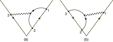
Figure 9: Vertex diagrams with fermionic propagators attached to the opposite edge of the gluon propagator.

Next we consider the case where the fermions are both attached to the same line, but the gluon is not. We have the two possibilities depicted in fig. 9. The diagram 9.(a) originates from the contribution (91) when considering the region of integration $-L\leq\tau_{3}\leq 0$ and $0\leq\tau_{2}\leq\tau_{1}\leq L$.

The diagram 9.(b) is instead obtained from (91), when $-L\leq\tau_{3}\leq\tau_{2}\leq 0$, $0\leq\tau_{1}\leq L$ and $\dot{x}_{3}=\dot{x}_{2}$. No contribution of this kind is instead contained in (91). Since the two graphs in fig. 9 are related by a reflection with respect to the axis bisecting the cusp, they yield the same result and thus we have to compute only one of them, e.g. 9.(a). For this diagram all the terms in (91), which are not proportional to $(\eta_{1}\bar{\eta}_{2})$, will vanish when we use that $\dot{x}_{1}=\dot{x}_{2}$ and so we get an expression that is similar to the one considered in (93a):

$$[\ref{Vertexb}.(a)]_{\rm up}=2N^{2}M\left(\frac{2\pi}{\kappa}\right)^{2}\int_{0}^{L}\!\!\!\!d\tau_{1}\int_{0}^{\tau_{1}}\!\!\!\!d\tau_{2}\int_{-L}^{0}\!\!\!\!d\tau_{3}~{}\dot{x}_{3\lambda}(\Gamma^{\tau\lambda\tau}-\Gamma^{\lambda\tau\tau}).$$ (99)

In order to compute this integral we first observe that the integrand can be rearranged as follows

$$\begin{split}&\dot{x}_{3\lambda}(\Gamma^{\tau\lambda\tau}-\Gamma^{\lambda\tau\tau})=\dot{x}_{3}\cdot\partial_{x_{2}}\Phi_{2,13}-\dot{x}_{3}\cdot\partial_{x_{1}}\Phi_{1,23}=\dot{x}_{3}\cdot\partial_{x_{2}}(\Phi_{2,13}+\Phi_{1,23})+\frac{d}{d\tau_{3}}\Phi_{1,23}\\ &=-\left(\frac{\Gamma(1/2-\epsilon)}{4\pi^{3/2-\epsilon}}\right)^{2}\frac{1}{(x^{2}_{13})^{1/2-\epsilon}}\frac{d}{d\tau_{3}}\frac{1}{(x^{2}_{23})^{1/2-\epsilon}}+\frac{d}{d\tau_{3}}\Phi_{1,23}.\end{split}$$ (100)

We have two separate contributions, which both appear in the list considered in appendix C (see eqs. (C.2) and (C.2)) and thus we can immediately write the final result

$$\!\!\![\ref{Vertexb}.(a)]_{\rm up}\!=-N^{2}M\left(\frac{2\pi}{\kappa}\right)^{2}L^{4\epsilon}\left(\frac{\Gamma(1/2-\epsilon)}{4\pi^{3/2-\epsilon}}\right)^{2}\biggl{[}\frac{1}{\epsilon}\left({\log\left(\cos\frac{\varphi}{2}\right)}-\frac{1}{2}\varphi\cot\varphi\right)\!+O(1)\biggr{]}.$$ (101)

The final set of diagrams that we have to consider are those where the two fermions end on different edges of the cusp. We have four possible graphs of this kind, which simply

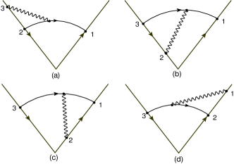
Figure 10: Vertex diagrams with fermionic propagators are attached to opposite edges.

differ for the position of the gluon line, and they are displayed in fig. 10. The diagrams 10.(a) and 10.(d) are obtained respectively from (91) and (91) when considering the region of integrations ${\rm(I)}=\{-L\leq\tau_{3}\leq\tau_{2}\leq 0$ and $0\leq\tau_{1}\leq L\}$ and ${\rm(II)}=\{-L\leq\tau_{3}\leq 0$ and $0\leq\tau_{2}\leq\tau_{1}\leq L\}$. The diagrams 10.(b) and 10.(c) originate instead from (91) when choosing either the range (I) or (II) for the parameters $\tau_{i}$. Again graphs, which are related by a reflection with respect the axis bisecting the cusp, produce the same result and we focus our attention only on 10.(a) and 10.(b).

To begin with, we shall factor out from both diagrams the color and $R-$symmetry dependence and we shall write

$$[\ref{Vertexc}.(a)]_{{\rm up}}\equiv-N^{2}M\left(\frac{2\pi}{\kappa}\right)^{2}\cos\frac{\theta}{2}~{}\mathcal{I}_{(a)}\ \ \ \ \ [\ref{Vertexc}.(b)]_{{\rm up}}\equiv-NM^{2}\left(\frac{2\pi}{\kappa}\right)^{2}\cos\frac{\theta}{2}~{}\mathcal{I}_{(b)}.$$ (102)

In order to simplify our analysis we shall construct the two independent combinations $\mathcal{I}_{(a)}-\mathcal{I}_{(b)}$ and $\mathcal{I}_{(a)}+\mathcal{I}_{(b)}$. The former is the only combination of the two integrals appearing in the final result when we would take the super-trace of the Wilson-loop and it is given by

$$\mathcal{I}_{(a)}-\mathcal{I}_{(b)}\!= \frac{2i}{(\eta_{2}\bar{\eta}_{1})}\int_{0}^{L}\!\!\!\!\!d\tau_{1}\!\!\int_{-L}^{0}\!\!\!\!\!d\tau_{2}\!\!\int_{-L}^{\tau_{2}}\!\!\!\!\!d\tau_{3}\!\left(\!\dot{x}_{1\nu}-(\dot{x}_{1}\cdot\dot{x}_{3})\dot{x}_{2\nu}-\frac{(\eta_{1}\bar{\eta}_{2})(\eta_{2}\bar{\eta}_{1})}{2}\dot{x}_{3\nu}\!\right)\!\left(\Gamma^{\tau\tau\nu}-\Gamma^{\tau\nu\tau}\right)\!=$$

$$= \frac{2i}{(\eta_{2}\bar{\eta}_{1})}\int_{0}^{L}\!\!\!\!d\tau_{1}\int_{-L}^{0}\!\!\!\!d\tau_{2}\int_{-L}^{\tau_{2}}\!\!\!\!d\tau_{3}\left(\dot{x}_{1\nu}+\dot{x}_{2\nu}\right)\left(\Gamma^{\tau\tau\nu}-\Gamma^{\tau\nu\tau}\right).$$ (103)

In (5.2.2) we were able to get rid of all the terms containing a three-point function contracted with three $\dot{x}_{i}$, thanks to the identity (B.158) and to the equality $\dot{x}_{2}=\dot{x}_{3}$, which holds for these diagrams. We can now use the relations (96) and the invariance under translation of the function $\Phi_{i,jk}$ to rewrite the integrand as follows

$$\begin{split}\left(\dot{x}_{1\nu}+\dot{x}_{2\nu}\right)\left(\Gamma^{\tau\tau\nu}-\Gamma^{\tau\nu\tau}\right)=&\frac{d}{d\tau_{3}}\Phi_{3,12}-\frac{d}{d\tau_{2}}\Phi_{2,13}-\frac{d}{d\tau_{1}}\Phi_{3,12}+\\ &+\left(\frac{\Gamma(1/2-\epsilon)}{4\pi^{3/2-\epsilon}}\right)^{2}\frac{1}{(x^{2}_{13})^{1/2-\epsilon}}\frac{d}{d\tau_{1}}\frac{1}{(x^{2}_{12})^{1/2-\epsilon}}.\end{split}$$ (104)

The integration over the circuit can be performed by means of the results given in app. C and we find

$$\mathcal{I}_{(a)}-\mathcal{I}_{(b)}\!= \frac{L^{4\epsilon}}{2\cos\frac{\varphi}{2}}\left(\frac{\Gamma(1/2-\epsilon)}{4\pi^{3/2-\epsilon}}\right)^{2}\left[\frac{1}{2\epsilon}\frac{\varphi}{\sin\varphi}+\frac{1}{\epsilon}\log\left(\cos\frac{\varphi}{2}\right)+\frac{1}{4\epsilon^{2}}-\right.$$ (105)

$$\left.-\frac{1}{\epsilon}\left(\frac{\varphi}{2}\cot\varphi-{\log\left(\cos\frac{\varphi}{2}\right)}\right)+\frac{1}{4\epsilon^{2}}+O(1)\right]=$$ (106)

$$= \left(\frac{\Gamma(1/2-\epsilon)}{4\pi^{3/2-\epsilon}}\right)^{2}\frac{{L^{4\epsilon}}}{4\epsilon}\frac{\varphi}{\sin\frac{\varphi}{2}}+O(1).$$ (107)

The sum $\mathcal{I}_{(a)}+\mathcal{I}_{(b)}$ is instead the only combination appearing in the final result if we take the trace of the loop operator. Its expression is less elegant than the one for the difference and it is given by

$$\mathcal{I}_{(a)}+\mathcal{I}_{(b)}=i\int_{0}^{L}\!\!\!\!\!d\tau_{1}\!\!\int_{-L}^{0}\!\!\!\!\!d\tau_{2}\!\!\int_{-L}^{\tau_{2}}\!\!\!\!\!d\tau_{3}~{}\Biggl{[}\frac{2}{(\eta_{2}\bar{\eta}_{1})}\biggl{(}2(\dot{x}_{1\nu}+\dot{x}_{3\nu})\Gamma^{\nu\tau\tau}+\dot{x}_{2\nu}\dot{x}_{1\lambda}\dot{x}_{3\sigma}\Gamma^{\nu\lambda\sigma}+$$

$$+\dot{x}_{2\lambda}\dot{x}_{1\sigma}\dot{x}_{3\nu}\Gamma^{\nu\lambda\sigma}-2\dot{x}_{1\nu}\dot{x}_{3\lambda}\dot{x}_{2\sigma}\Gamma^{\nu\lambda\sigma}\biggr{)}+(\eta_{1}\bar{\eta}_{2})~{}\dot{x}_{3\nu}(\Gamma^{\tau\nu\tau}+\Gamma^{\tau\tau\nu})\Biggr{]}.$$ (108)

It is not difficult to realize that the integrand in (5.2.2) is symmetric when exchanging $\tau_{2}$ with $\tau_{3}$: this allows us to extend the integration over $\tau_{3}$ up to $0$ provided dividing the result by two. We can reorganize (5.2.2) as follows

$$\mathcal{I}_{(a)}+\mathcal{I}_{(b)}= \frac{i}{2}\int_{0}^{L}\!\!\!\!\!d\tau_{1}\!\!\int_{-L}^{0}\!\!\!\!\!d\tau_{2}\!\!\int_{-L}^{0}\!\!\!\!\!d\tau_{3}~{}\Biggl{[}\frac{2}{(\eta_{2}\bar{\eta}_{1})}\biggl{(}2(\dot{x}_{1\nu}+\dot{x}_{3\nu})\Gamma^{\nu\tau\tau}+\dot{x}_{2\nu}\dot{x}_{1\lambda}\dot{x}_{3\sigma}\Gamma^{\nu\lambda\sigma}+$$

$$+\dot{x}_{2\lambda}\dot{x}_{1\sigma}\dot{x}_{3\nu}\Gamma^{\nu\lambda\sigma}-2\dot{x}_{1\nu}\dot{x}_{3\lambda}\dot{x}_{2\sigma}\Gamma^{\nu\lambda\sigma}\biggr{)}+(\eta_{1}\bar{\eta}_{2})~{}\dot{x}_{3\nu}(\Gamma^{\tau\nu\tau}+\Gamma^{\tau\tau\nu})\Biggr{]}=$$

$$= {i}\int_{0}^{L}\!\!\!\!\!d\tau_{1}\!\!\int_{-L}^{0}\!\!\!\!\!d\tau_{2}\!\!\int_{-L}^{0}\!\!\!\!\!d\tau_{3}~{}\Biggl{[}\frac{2}{(\eta_{2}\bar{\eta}_{1})}\biggl{(}(\dot{x}_{1\nu}+\dot{x}_{3\nu})\Gamma^{\nu\tau\tau}+\dot{x}_{2\nu}\dot{x}_{1\lambda}\dot{x}_{3\sigma}\Gamma^{\nu\lambda\sigma}-$$

$$-\dot{x}_{1\nu}\dot{x}_{3\lambda}\dot{x}_{2\sigma}\Gamma^{\nu\lambda\sigma}\biggr{)}+(\eta_{1}\bar{\eta}_{2})~{}\dot{x}_{3\nu}\Gamma^{\tau\tau\nu}\Biggr{]}.$$ (109)

In the second equality in (5.2.2) we have identified all the terms which differ by a permutation of $\tau_{2}$ with $\tau_{3}$, being trivially equivalent. We can distinguish two types of contributions: one containing only contracted three-point functions and the other where the three-point functions are saturated with three $\dot{x}_{i}$. The former can be rewritten in terms of the function $\Phi_{i,jk}$ by means of the relations (96) and we obtain

$${i}\int_{0}^{L}\!\!\!\!\!d\tau_{1}\!\!\int_{-L}^{0}\!\!\!\!\!d\tau_{2}\!\!\int_{-L}^{0}\!\!\!\!\!d\tau_{3}~{}\Biggl{[}\frac{2}{(\eta_{2}\bar{\eta}_{1})}(\dot{x}_{1\nu}+\dot{x}_{3\nu})\Gamma^{\nu\tau\tau}+(\eta_{1}\bar{\eta}_{2})~{}\dot{x}_{3\nu}\Gamma^{\tau\tau\nu}\Biggr{]}=$$

$$= {i}\int_{0}^{L}\!\!\!\!\!d\tau_{1}\!\!\int_{-L}^{0}\!\!\!\!\!d\tau_{2}\!\!\int_{-L}^{0}\!\!\!\!\!d\tau_{3}~{}\Biggl{[}\frac{2}{(\eta_{2}\bar{\eta}_{1})}\biggl{(}\frac{d}{d\tau_{1}}\Phi_{1,23}-\frac{d}{d\tau_{2}}\Phi_{1,23}-\frac{d}{d\tau_{3}}\Phi_{1,23}\biggr{)}+(\eta_{1}\bar{\eta}_{2})\frac{d}{d\tau_{3}}\Phi_{3,12}\Biggr{]}.$$ (110)

The divergent part of these integrals can be extracted from the table of integrals presented in app. C and we find

$$\frac{\Gamma^{2}(1/2-\epsilon)}{16\pi^{3-2\epsilon}}\left[\frac{L^{4\epsilon}}{\cos\frac{\varphi}{2}}\left[\frac{2}{\epsilon}\log\left(\sec\left(\frac{\varphi}{2}\right)+1\right)-\frac{1}{2\epsilon^{2}}\right]+\frac{L^{4\epsilon}}{\epsilon}\cos\frac{\varphi}{2}\log\left(\cos\frac{\varphi}{2}\right)+O(1)\right].$$ (111)

The procedure for determining the divergences of the latter contribution in (5.2.2) is more delicate, since we have to deal with the untraced three-point function. After a careful analysis, one gets

$$\frac{2i}{(\eta_{2}\bar{\eta}_{1})}\int_{0}^{L}\!\!\!\!\!d\tau_{1}\!\!\int_{-L}^{0}\!\!\!\!\!d\tau_{2}\!\!\int_{-L}^{0}\!\!\!\!\!d\tau_{3}~{}\biggl{(} \dot{x}_{2\nu}\dot{x}_{1\lambda}\dot{x}_{3\sigma}\Gamma^{\nu\lambda\sigma}-\dot{x}_{1\nu}\dot{x}_{3\lambda}\dot{x}_{2\sigma}\Gamma^{\nu\lambda\sigma}\biggr{)}=$$

$$=-\frac{\Gamma^{2}(1/2-\epsilon)}{16\pi^{3-2\epsilon}}\frac{{L^{4\epsilon}}}{\epsilon}\cos\frac{\varphi}{2}\log\left(\cos\frac{\varphi}{2}\right)+O(1).$$ (112)

If we sum (111) and (5.2.2), we can finally write down the result for $\mathcal{I}_{(a)}+\mathcal{I}_{(b)}$

$$\mathcal{I}_{(a)}+\mathcal{I}_{(b)}=\frac{\Gamma^{2}(1/2-\epsilon)}{16\pi^{3-2\epsilon}}\frac{L^{4\epsilon}}{\cos\frac{\varphi}{2}}\left[\frac{2}{\epsilon}\log\left(\sec\left(\frac{\varphi}{2}\right)+1\right)-\frac{1}{2\epsilon^{2}}\right]+O(1).$$ (113)

This completes the evaluation of the divergent part of all diagrams at two loops.

6 The final result: summing and renormalizing

In this section we shall add up the different diagrams which appear at two loops. Because we are actually working with an open contour, we have in principle two possibilities to perform this sum: we can take the trace [$\mathcal{W}_{+}$ in (24)] or the super-trace [$\mathcal{W}_{-}$ in (24)]. As we shall see, the first choice, that is the correct one for closed contours, appears to be consistent with an exponentiated form. We also discuss the renormalization of our result, paying particular attention to the peculiarities arising in three dimensions and in the presence of the exotic fermionic couplings.

6.1 Taking the trace

Let us consider the case of the trace. The bosonic bubble diagrams yield a four-dimensional-like contribution given by

$$\mathds{B}=-g(\epsilon)\left(\cos\varphi-\cos^{2}\frac{\theta}{2}\right)\frac{1}{\epsilon}\frac{\varphi}{\sin\varphi},$$ (114)

where we have introduced the short-hand notation

$$g(\epsilon)=MN\left(\frac{2\pi}{\kappa}\right)^{\!\!2}\!\frac{\Gamma^{2}\!\left(\frac{1}{2}-\epsilon\right)}{16\pi^{3-2\epsilon}}(\mu L)^{4\epsilon}$$ (115)

for future convenience. The fermionic bubble instead cancels when we take the trace, since it is odd in the exchange $N\leftrightarrow M$. The total result for the complete set of double-exchange diagrams is more elaborate and it can be usefully cast in the form

$$\begin{split}\mathds{D}=&2g(\epsilon)\Biggl{[}\frac{1}{\epsilon^{2}}\left[2-\frac{3}{2}\frac{\cos\frac{\theta}{2}}{\cos\frac{\varphi}{2}}\right]+\frac{1}{\epsilon}\left[\frac{\cos\frac{\theta}{2}}{\cos\frac{\varphi}{2}}\left(4\log\left(\sec\frac{\varphi}{2}+1\right)+\log\left(\cos\frac{\varphi}{2}\right)\right)+1\right]+\\ &+\frac{1}{4}\left[\frac{\cos\frac{\theta}{2}}{\cos\frac{\varphi}{2}}\left(\frac{1}{\epsilon}-2\log\left(1+\sec\frac{\varphi}{2}\right)\right)\right]^{2}-\frac{1}{2\epsilon}\cos^{2}\frac{\theta}{2}\frac{\varphi}{\sin\varphi}+O(1)\Biggr{]}.\end{split}$$ (116)

The diagrams which contain the gauge-fermion interaction yield instead the following result

$$\mathds{V}\!=\!\frac{g(\epsilon)}{\epsilon^{2}}\!\left[{\frac{\cos\frac{\theta}{2}}{\cos\frac{\varphi}{2}}-2}\right]+\frac{g(\epsilon)}{\epsilon}\!\left[{\varphi\cot\varphi-2\!\left(\!2\frac{\cos\frac{\theta}{2}}{\cos\frac{\varphi}{2}}\log\left(\sec\frac{\varphi}{2}+1\right)+\log\left(\cos\frac{\varphi}{2}\right)\!+\!1\!\right)}\right]\!+\!O\left(1\right)\!.$$ (117)

We shall now sum these three contributions in order to obtain the unrenormalized value of $\mathcal{W}_{+}$ in (24) at two loops

$$\begin{split}[\mathcal{W}_{+}]_{\rm 2-loop}=&\frac{g(\epsilon)}{2\epsilon^{2}}\left(\frac{\cos\frac{\theta}{2}}{\cos\frac{\varphi}{2}}-2\right)^{2}+\frac{2g(\epsilon)}{\epsilon}\frac{\cos\frac{\theta}{2}}{\cos\frac{\varphi}{2}}\left(2-\frac{\cos\frac{\theta}{2}}{\cos\frac{\varphi}{2}}\right)\log\left(\sec\frac{\varphi}{2}+1\right)+\\ &\ \ \ \ \ \ \ \ \ \ \ \ \ \ \ +\frac{2g(\epsilon)}{\epsilon}\log\left(\cos\frac{\varphi}{2}\right)\left(\frac{\cos\frac{\theta}{2}}{\cos\frac{\varphi}{2}}-1\right)+O(1).\end{split}$$ (118)

In this expression the structure of the generalized potential is not manifest. Crucially we observe the presence of double-poles that are not expected to appear in the final expression of the generalized potential. In conventional Wilson loops, where only bosonic couplings are concerned, double-poles at two loops are simply understood as coming from the square of the one-loop result, by virtue of the non-abelian exponentiation theorem Exp (that holds even at renormalized level). The non-trivial contribution at second order in perturbation theory comes from the so-called maximally non-abelian part and in ${\cal N}=4$ SYM, for example, involves crossed non-planar bosonic exchanges and interacting diagrams, stretching between the two lines. In our case, due to the presence of the fermionic couplings, we do not have an established exponentiation theorem at hand and we were forced to compute the full two-loop contribution to the quantum average. Incidentally, for our loops, double-poles appear both from exchange and interacting diagrams at variance with ${\cal N}=4$ SYM, where non-abelian exponentiation forbids the presence of $1/\epsilon^{2}$ in vertex or bubble graphs. In order to proceed and extract a generalized potential, taking properly into account the one-loop and two-loop results, we need an exponentiation ansatz: we propose the following form for the unrenormalized loop

$$\mathcal{W}_{+}=\frac{M\exp(V_{N})+N\exp(V_{M})}{N+M}.$$ (119)

It is not difficult to check that our results are compatible with this double-exponentiation where

$$V_{N}= \left(\frac{2\pi}{\kappa}\right)N\left(\frac{\Gamma(1/2-\epsilon)}{4\pi^{3/2-\epsilon}}\right)(\mu L)^{2\epsilon}\left[\frac{1}{\epsilon}\left(\frac{\cos\frac{\theta}{2}}{\cos\frac{\varphi}{2}}-2\right)-2\frac{\cos\frac{\theta}{2}}{\cos\frac{\varphi}{2}}\log\left(\sec\left(\frac{\varphi}{2}\right)+1\right)\right]+$$

$$+N^{2}\left(\frac{2\pi}{\kappa}\right)^{\!\!2}\!\frac{\Gamma^{2}\!\left(\frac{1}{2}-\epsilon\right)}{16\pi^{3-2\epsilon}}(\mu L)^{4\epsilon}\left[\frac{1}{\epsilon}\log\left(\cos^{2}\frac{\varphi}{2}\right)\left(\frac{\cos\frac{\theta}{2}}{\cos\frac{\varphi}{2}}-1\right)+O(1)\right]$$ (120)

The generalized potential $V_{M}$ is of course obtained by exchanging $M$ with $N$ in the above formula. We remark that the actual exponentiation of the one-loop term is a non-trivial support of our assumption and of the correctness of our computations, involving a delicate balance between exchanging and interacting contributions. From the physical point of view we could also justify the presence of two generalized potentials, simply recalling that we have two different test particles running in our contour. Following Lee:2010hk it is straightforward to show that in $U(N)\times U(M)$ ${\cal N}=6$ theories two kinds of particles arise from the relevant higgsing procedure and which transform respectively in the $({\bf N},{\bf 1})$ and $({\bf 1},{\bf M})$ representations and their conjugate, that we call $W_{N}$ and $W_{M}$ bosons. It is clear that a pair of $W_{N}$ and $W_{M}$ cannot form a singlet of the color indices and there is no generalization of the quark-antiquark potential in this case. On the other hand a pair of $W_{N}\bar{W}_{N}$ or $W_{M}\bar{W}_{M}$ do form color singlets, hence there are two potentials in this theory.

6.2 The renormalized generalized potentials

The outcome of our extensive two-loop computation contains some puzzling unexpected features which deserve a more detailed analysis. To begin with, let us consider the one-loop contribution in (6.1). When $\theta=\varphi=0$ our cusp degenerates into a segment of length $2L$ with the couplings of the $1/2$ BPS straight line and its (unrenormalized) value is given at the first non-trivial order by

$${W}^{(1)}_{\rm line}= -\left(\frac{2\pi}{\kappa}\right)\frac{MN}{N+M}\left(\frac{\Gamma(1/2-\epsilon)}{4\pi^{3/2-\epsilon}}\right)(\mu L)^{2\epsilon}\left[\frac{1}{\epsilon}+2\log\left(2\right)+O(\epsilon)\right]=$$

$$= -\left(\frac{2\pi}{\kappa}\right)\frac{MN}{N+M}\left(\frac{\Gamma(1/2-\epsilon)}{4\pi^{3/2-\epsilon}}\right)\frac{(2L\mu)^{2\epsilon}}{\epsilon}+O(\epsilon).$$ (121)

This divergent result appears to contradict the expectation that the $1/2-$BPS straight-line is trivial (i.e. equal to $1$) as occurs in $\mathcal{N}=4$ SYM. In that case an analogous computation for a segment of length $2L$ in Feynman gauge would have led to an exact cancellation between the gauge and the scalar contribution yielding as final result $W^{(1)}_{\rm line}=0$. We remark, however, that this manifest zero in $\mathcal{N}=4$ SYM is peculiar of the Feynman gauge. In a generic $\alpha-$gauge the cancellation is only partial and a divergent term similar to (6.2) survives,

$$W^{(1)}_{\rm line}=g^{2}N(1-\alpha)\frac{\Gamma(1-\epsilon)}{16\pi^{2-\epsilon}}\frac{(2L\mu)^{\epsilon}}{\epsilon}.$$ (122)

The $\alpha-$dependence in (122) signals that we are dealing with a gauge-dependent divergence, but this is not surprising. In fact the result (122) is the expectation value for a segment of length $2L$, which does not define a gauge invariant operator unless $L=\infty$. However the limit $L\to\infty$ is delicate and it cannot be taken before renormalizing the finite length operator.

The systematic renormalization of Wilson operator on open contours is a subject widely discussed in the literature Dorn1 ; Dorn2 ; Aoyama:1981ev ; Knauss:1984rx ; Dorn:1986dt and an exhaustive presentation of the topic is beyond the goal of this paper. Below we shall recall some general facts using YM or $\mathcal{N}=4$ SYM as our pedagogical examples. The case of ABJM will be considered later.

An efficient frame-work for discussing the renormalization of path ordered phase factors was introduced by Arefeva:1980zd ; Gervais:1979fv . In this approach these non-local operators are represented as the two point function $\left\langle\psi(-L)\bar{\psi}(L)\right\rangle_{0}$ of the one-dimensional fermionic bare action

$$S=\int_{-L}^{L}\!\!dt~{}\bar{\psi}(i\partial_{t}+g\mathcal{A}_{\mu}\dot{x}^{\mu})\psi,$$ (123)

where $\mathcal{A}_{\mu}$ stands for the connection of which we are computing the quantum holonomy. The familiar techniques of renormalization for local Green function can be therefore applied.

In this language the divergence (122) is responsible for the familiar wave-function renormalization of the field $\psi$ and it can be in fact eliminated by introducing $\psi_{R}=Z^{-1/2}_{\psi}\psi$. This interpretation is also consistent with the fact that its value is gauge-dependent. The usual perimeter divergence, present in a cut-off regularization, appears as a mass counter-term for the spinor $\psi$ in the renormalized action.

According to the previous discussion, the renormalized operator for an open smooth contour $C$ is obtained as Dorn1 ; Dorn2 ; Aoyama:1981ev ; Knauss:1984rx ; Dorn:1986dt

$$\begin{split}{\cal W}_{\rm ren.}=&\left\langle\psi_{R}(-L)\bar{\psi}_{R}(L)\right\rangle_{0}=\\ =&Z^{-1}_{\psi}\left\langle\psi(-L)\bar{\psi}(L)\right\rangle_{0}=Z^{-1}_{\psi}e^{-\ell\delta m}\left\langle P\exp\left(ig_{\rm ren.}\frac{Z_{1}}{Z_{3}}\int_{C}dx^{\mu}\mathcal{A}^{\rm ren.}_{\mu}\right)\right\rangle_{0},\end{split}$$ (124)

where $Z_{1}$ and $Z_{3}$ are the usual renormalization for the gauge coupling constant and the wave-function renormalization for $\mathcal{A}_{\mu}$. Moreover $\ell$ is the perimeter of the smooth open contour $C$; the mass renormalization $\delta m$ is zero when dimensional regularization is used since it corresponds to a power-like divergence.

An important remark is now in order. In dimensional regularization the new renormalization constant $Z_{\psi}$ can be shown to be independent of the shape of the smooth contour Dorn1 ; Dorn2 ; Aoyama:1981ev ; Knauss:1984rx ; Dorn:1986dt (up to a redefinition of the renormalization scale). Accordingly its value can be computed for a finite segment and then used for other smooth contours.

When we close the circuit, thus considering a Wilson loop, a new divergence appears Dorn1 ; Dorn2 ; Aoyama:1981ev ; Knauss:1984rx ; Dorn:1986dt , since the two fields in $\left\langle\psi(-L)\bar{\psi}(L)\right\rangle_{0}$ are now located at the same point. More correctly the closed loop does not define a two-point function, but the expectation value of a composite operator: this explains the need of a further renormalization. However the effect of this additional ingredient is to exactly cancel the factor $Z^{-1}_{\psi}$ Dorn1 ; Dorn2 ; Aoyama:1981ev ; Knauss:1984rx ; Dorn:1986dt and one recovers the familiar and simple result

$$\begin{split}{\cal W}^{\rm clos.~{}loop}_{\rm ren.}=e^{-\ell\delta m}\left\langle P\exp\left(ig_{\rm ren.}\frac{Z_{1}}{Z_{3}}\oint_{C}dx^{\mu}\mathcal{A}^{\rm ren.}_{\mu}\right)\right\rangle_{0},\end{split}$$ (125)

i.e. a smooth Wilson loop does not contain any new divergence with respect to those of the gauge theory, apart from the one proportional to the perimeter of the contour. Since $Z_{\psi}$ is only present when dealing with open circuits, but disappears for closed loops, it is also named $Z_{\rm open}$.

Let us remark that the final equalities in (124) and (125) define a procedure for renormalizing smooth path ordered phase factors independently of the fermionic representation used to prove them.

We come back to the example of the segment in $\mathcal{N}=4$ SYM. If we introduce the wave-function renormalization

$$Z_{\rm open}=1+g^{2}N(1-\alpha)\frac{\Gamma(1-\epsilon)}{16\pi^{2-\epsilon}}\frac{(2L\mu)^{\epsilon}}{\epsilon}.$$ (126)

the expectation value of the renormalized operator becomes again trivial as occurs in Feynman gauge. In the case of ABJM, the divergence can be handled in the same way by introducing

$$Z_{\rm open}= 1-\left(\frac{2\pi}{\kappa}\right)\frac{MN}{N+M}\left(\frac{\Gamma(1/2-\epsilon)}{4\pi^{3/2-\epsilon}}\right)\frac{(2L\mu)^{2\epsilon}}{\epsilon}+O(\epsilon).$$ (127)

In other words, with respect to the familiar $\mathcal{N}=4$ result ($\alpha=1$), the Landau gauge used to compute (6.2) in ABJM theories does not enjoy the simplifying property $Z_{\rm open}=1$.

Let us now turn to piecewise smooth contours Polyakov:1980ca ; Korchemsky:1987wg ; Dorn1 ; Dorn2 ; Knauss:1984rx ; Dorn:1986dt , namely to contours containing points where the derivative $\dot{x}^{\mu}$ is discontinuous. If there is a cusp at $t=t_{0}$, i.e. $\lim_{t\to t_{0}^{+}}\dot{x}^{\mu}(t)\neq\lim_{t\to t_{0}^{-}}\dot{x}^{\mu}(t)$, the renormalization of the action (123) requires an additional counter-term proportional to $\bar{\psi}(t_{0})\psi(t_{0})$ Knauss:1984rx ; Dorn:1986dt . To argue the origin of this new counter-term we observe that a reasonable renormalization procedure should respect the composition rule for path-ordered phase factors on smooth contours. Specifically if we split a regular contour $C$ $\{x(t)|-L\leq t\leq L\}$ into two sub-contours $C_{1}$ $\{x(t)|-L\leq t\leq t_{0}\}$ and $C_{2}$ $\{x(t)|t_{0}\leq t\leq L\}$

$$\mathcal{W}^{\rm ren.}(C_{1})\mathcal{W}^{\rm ren.}(C_{2})=W^{\rm ren.}(C).$$ (128)

In terms of the two point function of the one-dimensional fermion $\psi$ this property reads

$$\langle\psi(-L)\bar{\psi}(t_{0})\rangle\langle\psi(t_{0})\bar{\psi}(L)\rangle=\langle\psi(-L)(\bar{\psi}\psi)(t_{0})\bar{\psi}(L)\rangle=\langle\psi(-L)\bar{\psi}(L)\rangle.$$ (129)

The intermediate equality implies that the renormalization factor $Z_{\bar{\psi}\psi}$ for the composite operator $(\bar{\psi}\psi)(t_{0})$ is $1$. This is an equivalent manifestation of the previous statement that $Z_{\rm open}$ drops out when the two endpoints of a loop are joined smoothly. If $t_{0}$ is instead the position of a cusp the factor $Z_{\bar{\psi}\psi}$ can be in general different from $1$ and it must be included in the renormalization of the Wilson-operator. Its insertion leads to the following modification of (124) for open contour with one cusp Dorn1 ; Dorn2 ; Knauss:1984rx ; Dorn:1986dt

$$\begin{split}{\cal W}_{\rm ren.}=Z^{-1}_{\rm open}Z_{\bar{\psi}\psi}e^{-\ell\delta m}\left\langle P\exp\left(ig_{\rm ren.}\frac{Z_{1}}{Z_{3}}\int_{C}dx^{\mu}\mathcal{A}^{\rm ren.}_{\mu}\right)\right\rangle_{0}.\end{split}$$ (130)

In the following we shall replace the symbol $Z_{\bar{\psi}\psi}$ with the more familiar $Z_{\rm cusp}$.

The renormalization factor $Z_{\rm cusp}$ can be shown to depend only on the angle $\varphi$ of the cusp and not on the global geometry of the circuit, and to be gauge invariant. Moreover it must satisfy a simple renormalization condition Dorn2 ; Knauss:1984rx ; Dorn:1986dt

$$\left.Z_{\rm cusp}\right|_{\varphi=0}=1,$$ (131)

since the cusp disappears for $\varphi=0$ and no new renormalization is needed apart from $Z_{\rm open}$. This condition also appears in Korchemsky:1987wg as a Ward identity for the vertex in the one-dimensional field theory. The new factor will give origin to the well-known cusp-anomalous dimension, which is defined through the relation

$$\gamma=\mu\frac{d}{d\mu}\log Z_{\rm cusp}.$$ (132)

We expect that the above renormalization procedure carries over to the case of the Wilson loop in ABJ theory with minor changes. In fact the structure of eq. (130) is substantially independent of the specific form of $\mathcal{A}_{\mu}$ and of the route used to prove it. A detailed proof of the above results, in the case of the phase operator defined by the super-connection (9), could be obtained by using the supersymmetric quantum mechanics discussed in Lee:2010hk as a starting point instead of (123). An obvious difference with the above discussion arises when considering the renormalization condition. For our operators eq. (131) must be replaced by

$$\left.Z_{\rm cusp}\right|_{\varphi=\theta=0}=1.$$ (133)

Recall, in fact, that we have also a cusp in the $R-$symmetry directions governed by the angle $\theta$ next to geometrical one given by $\varphi$. In this language the BPS condition $\theta=\varphi$ should translate into the following

$$\left.Z_{\rm cusp}\right|_{\varphi=\theta}=1.$$ (134)

Eq. (134) is not equivalent to (133). Thus the BPS condition still provides a check of the correctness of our computation.

Having in mind the above discussion, it is straightforward to extract the renormalized generalized potential $V^{\rm Ren.}_{N}$ from (6.1). We obtain

$$\!\!V^{\rm Ren.}_{N}= \left(\frac{2\pi}{\kappa}\right)N\left(\frac{\Gamma(\frac{1}{2}-\epsilon)}{4\pi^{3/2-\epsilon}}\right)\!(\mu L)^{2\epsilon}\!\!\left[\frac{1}{\epsilon}\left(\frac{\cos\frac{\theta}{2}}{\cos\frac{\varphi}{2}}-1\right)\!\!-2\frac{\cos\frac{\theta}{2}}{\cos\frac{\varphi}{2}}\log\left(\sec\left(\frac{\varphi}{2}\right)\!+\!1\right)\!\!+\log 4\right]\!+$$

$$+\left(\frac{2\pi}{\kappa}\right)^{\!\!2}N^{2}\!\left(\frac{\Gamma\!\left(\frac{1}{2}-\epsilon\right)}{4\pi^{3/2-\epsilon}}\right)^{2}(\mu L)^{4\epsilon}\left[\frac{1}{\epsilon}\log\left(\cos\frac{\varphi}{2}\right)^{2}\left(\frac{\cos\frac{\theta}{2}}{\cos\frac{\varphi}{2}}-1\right)+O(1)\right],$$ (135)

where we have included the finite terms for completeness. The terms proportional to $1/\epsilon$ give the logarithm of the celebrated $Z_{\rm cusp}$. It is trivial to check that $\left.Z_{\rm cusp}\right|_{\varphi=\theta}=1$.

The quark-antiquark potential is recovered by taking the limit $\varphi\to\pi$ and following the prescription of Drukker:2011za

$$V^{(s)}_{N}(R)=\frac{N}{k}\frac{1}{R}-\left(\frac{N}{k}\right)^{2}\frac{1}{R}\log\left(\frac{T}{R}\right).$$ (136)

We observe a logarithmic, non-analytic term in $T/R$ at the second non-trivial order that, as in four dimensions, is expected to disappear when resummation of the perturbative series is performed. We can also perform the opposite limit, taking large imaginary $\varphi$, and we recover the universal cusp anomaly

$$\gamma_{cusp}=\frac{N^{2}}{k^{2}},$$ (137)

that is the result obtained directly from the light-like cusp Henn:2010ps .

6.3 $1/2-$BPS line versus $1/6-$BPS line

In the previous subsection we have discussed the appearence of spurious divergences in the quantum computation of our cusped Wilson loops and explained their subtraction procedure: we have also remarked that these divergences obstinately persits in the case of $1/2-$BPS straight-lines, although not contradicting their triviality. However there is still an additional feature that may appear puzzling. In Drukker:2009hy it was pointed out that the $1/2-$BPS straight-line is cohomologically equivalent to its $1/6-$BPS counterpart, defined in Drukker:2008zx . One can easily show that, at least at one loop, the expectation value of the latter is trivial without requiring any renormalization, exactly as in ${\cal N}=4$: encountering divergences in the evaluation of $1/2-$BPS straight-line seems therefore to contradict the cohomological equivalence.

The key point of Drukker:2009hy , in order to establish the equivalence of the two observables, was to observe that the difference between $\mathcal{W}^{1/2}_{\rm line}$ and $\mathcal{W}^{1/6}_{\rm line}$ can be cast into a $Q-$exact term

$$\mathcal{W}^{1/2}_{\rm line}-\mathcal{W}^{1/6}_{\rm line}=QV,$$ (138)

where the supercharge $Q$ is that generated by the spinor $\bar{\theta}^{IJ\beta}=(\bar{n}^{I}\bar{w}^{J}-\bar{n}^{J}\bar{w}^{I})\bar{\eta}^{\beta}-i\epsilon^{IJKL}n_{K}w_{L}\eta^{\beta}$, while the scalar couplings in $\mathcal{W}^{1/6}_{\rm line}$ are governed by the matrices $M_{J}^{\ \ I}=\widehat{M}_{J}^{\ \ I}=\delta^{I}_{J}-2n_{J}\bar{n}^{I}-2w_{J}\bar{w}^{I}.$ A complete expression for $V$ has been presented in Drukker:2009hy , but we shall not report it here. To understand why the above identity fails, it will suffice to consider its lowest non trivial order in $1/k$: using the notation of Drukker:2009hy we explicitly obtain

$${\small\begin{split}-i\int_{-\infty}^{\infty}\!\!\!\!\!\!dt~{}\tilde{\mathcal{L}}_{B}-\int_{-\infty}^{\infty}\!\!\!\!\!\!dt_{1}\int_{-\infty}^{t_{1}}\!\!\!\!\!\!dt_{2}\mathcal{L}_{F}(t_{1})\mathcal{L}_{F}(t_{2})=-\frac{1}{2}Q\left(\int_{-\infty}^{\infty}\!\!\!\!\!\!dt_{1}\int_{-\infty}^{t_{1}}\!\!\!\!\!\!dt_{2}[\Lambda(\tau_{1})\mathcal{L}_{F}(\tau_{2})-\mathcal{L}_{F}(\tau_{1})\Lambda(\tau_{2}))]\!\right)\!\!.\end{split}}$$ (139)

The quantities $\tilde{\mathcal{L}}_{B},~{}\mathcal{L}_{F}$ and $\Lambda$ in (139) are defined by the following matrices

$${\small\begin{split}\!\!\!\tilde{\mathcal{L}}_{B}=-\frac{4\pi i}{k}|\dot{x}|\begin{pmatrix}C_{\bar{w}}\bar{C}^{w}&0\\ 0&\bar{C}^{w}C_{\bar{w}}\end{pmatrix}\ \ \mathcal{L}_{F}=-i\sqrt{\frac{2\pi}{k}}|\dot{x}|\begin{pmatrix}0&\eta\bar{\psi}\\ \psi\bar{\eta}&0\end{pmatrix}\ \ \Lambda=-\frac{1}{2}\sqrt{\frac{2\pi}{k}}|\dot{x}|\begin{pmatrix}0&i\bar{C}^{w}\\ C_{\bar{w}}&0\end{pmatrix}\end{split}}$$ (140)

where the scalars are given by $C_{\bar{w}}=\bar{w}^{I}C_{I}$ and $\bar{C}^{w}=\bar{C}^{J}w_{J}$, the reduced spinors are written as $\bar{\psi}=\bar{\psi}^{I}n_{I}$ and $\psi=\psi_{I}\bar{n}^{I}$.

When we replace the infinite straight-line with a segment of length $2L$ to tame the infrared divergences, the above equality receives a correction from the value of the scalar fields on the boundary. Taking properly into account some total derivatives, usually discarded for infinite lenght, (139) is replaced by

$${\small\begin{split}\int_{-\infty}^{\infty}\!\!\!\!\!\!dt~{}&\tilde{\mathcal{L}}_{B}+\int_{-\infty}^{\infty}\!\!\!\!\!\!dt_{1}\int_{-\infty}^{t_{1}}\!\!\!\!\!\!dt_{2}\mathcal{L}_{F}(t_{1})\mathcal{L}_{F}(t_{2})+4i\int_{-L}^{L}\!\!\!\!dt\left(\frac{\Lambda(L)\Lambda(t)}{|\dot{x}_{L}|}+\frac{\Lambda(t)\Lambda(-L)}{|\dot{x}_{-L}|}\right)=\\ &=-\frac{1}{2}Q\left(\int_{-L}^{L}\!\!\!\!\!\!dt_{1}\int_{-L}^{t_{1}}\!\!\!\!\!\!dt_{2}[\Lambda(\tau_{1})\mathcal{L}_{F}(\tau_{2})-\mathcal{L}_{F}(\tau_{1})\Lambda(\tau_{2}))]\!\right).\end{split}}$$ (141)

In other words, if defined on a segment the two Wilson operator are not cohomologically equivalent! Actually we can go further and observe that the divergence of the $1/2-$BPS line comes entirely from these boundary terms, when evaluated at quantum level. For instance it is easy to check that the new term in (141) is accountable for the result (6.2). The renormalization procedure described in the previous subsection is built to subtract exactly these spurious contributions.

7 Conclusions and outlook

In this paper we have studied a family of cusped Wilson loops in ABJ(M) super Chern-Simons theory, constructed from two 1/2 BPS lines implying the presence of peculiar fermionic couplings Drukker:2009hy . They depend on two parameters, $\varphi$ and $\theta$, that describe the geometrical and $R$-symmetry angles, respectively, between the two rays. We have studied the supersymmetric properties of these configurations and their relation with closed contours, obtained through conformal transformations. Different limits on the parameters allow to reach interesting observables, as the analogous of the quark-antiquark potential or the universal cusp anomalous dimension. We have performed an explicit two-loop computation in dimensional regularization and we have obtained the divergent part of these contour operators. Our results suggest the existence of two generalized potentials in this theory and, after renormalization, we have obtained in the relevant limits the universal cusp anomaly and the $W_{N(M)}\bar{W}_{N(M)}$ binding energy.

The construction of a generalized potential from a cusped Wilson loop opens many interesting possibilities in ABJ(M) theory: one could try to compute the radiation of a particle moving along an arbitrary smooth path, as done in ${\cal N}=4$ SYM Correa:2012at . Further, one could hope to find a three dimensional analogue of the set of TBA integral equations, recently discovered in Drukker:2012de ; Correa:2012hh , describing non-perturbatively the D=4 generalized cusp (see also Bykov:2012sc ; Henn:2012qz ; Gromov:2012eu for very recent developments). It is also tempting to speculate on the possibility to derive the infamous interpolating function $h(\lambda)$ H ; Grignani:2008is ; Nishioka:2008gz ; BT1 ; BT2 ; MZ ; GGY , by comparing the integrability computations with exact results obtained through localization Kapustin:2009kz . An important step in this program would be the derivation of general class of Wilson loops with lower degree of supersymmetry, specifically some analogue of the DGRT loops Drukker:2007qr in ${\cal N}=6$ super Chern-Simons theory. A particular case, the wedge on $S^{2}$, has been discussed here in sec. 3: a general construction of BPS loops on $S^{2}$, preserving fractions of supersymmetry, will be presented soon CGMS . It would be of course important to compute their quantum expectation value at weak coupling, by perturbation theory, and at strong coupling, using string techniques. Hopefully their exact expression could be derived through localization methods.

Appendix A Basics of ABJ(M) action

Here we will collect some basic facts about the ABJ(M) action in Euclidean space-time. The gauge sector consists of two gauge fields $(A_{\mu})_{i}^{\ j}$ and $(\hat{A}_{\mu})_{\hat{i}}^{\ \hat{j}}$ belonging respectively to the adjoint of $U(N)$ and $U(M)$. The matter sector instead contains the complex fields $(C_{I})_{i}^{\ \hat{i}}$ and $({\bar{C}}^{I})_{\hat{i}}^{\ i}$ as well as the fermions $(\psi_{I})_{\hat{i}}^{\ i}$ and $({\bar{\psi}}^{I})_{i}^{\ \hat{i}}$. The fields $(C,\bar{\psi})$ transform in the $({\bf N},{\bf\bar{M}})$ of the gauge group $U(N)\times U(M)$ while the couple $(\bar{C},\psi)$ lives in the $({\bf\bar{N}},{\bf M})$. The additional capitol index $I=1,2,3,4$ belongs to the $R-$symmetry group $SU(4)$. In order to quantize the theory at the perturbative level, we have introduced the covariant gauge fixing function $\partial_{\mu}A^{\mu}$ for both gauge fields and two sets of ghosts $(\bar{c},c)$ and $(\bar{\hat{c}},\hat{c})$. Therefore we work with the following Euclidian space action (see Chen:1992ee ; Aharony:2008ug ; Benna:2008zy )

$$S_{\text{CS}} =-i\frac{k}{4\pi}\,\int d^{3}x\,\varepsilon^{\mu\nu\rho}\,\Bigl{[}\,\mathrm{Tr}(A_{\mu}\partial_{\nu}A_{\rho}+\frac{2}{3}\,A_{\mu}A_{\nu}A_{\rho})-\mathrm{Tr}(\hat{A}_{\mu}\partial_{\nu}\hat{A}_{\rho}+\frac{2}{3}\,\hat{A}_{\mu}\hat{A}_{\nu}\hat{A}_{\rho})\,\Bigr{]}$$

$$S_{\text{gf}} =\frac{k}{4\pi}\,\int d^{3}x\,\Bigl{[}\,\frac{1}{\xi}\,\mathrm{Tr}(\partial_{\mu}A^{\mu})^{2}+\mathrm{Tr}(\partial_{\mu}\bar{c}\,D_{\mu}c)-\frac{1}{\xi}\,\mathrm{Tr}(\partial_{\mu}\hat{A}^{\mu})^{2}+\mathrm{Tr}(\partial_{\mu}\bar{\hat{c}}\,D_{\mu}\hat{c})\,\Bigr{]}$$

$$S_{\text{Matter}} =\int d^{3}x\,\Bigl{[}\,\mathrm{Tr}(D_{\mu}\,C_{I}\,D^{\mu}{\bar{C}}^{I})+i\,\mathrm{Tr}(\bar{\psi}^{I}\,{D}\!\!\!\!/\,\,\psi_{I})\,\Bigr{]}+S_{\text{int}}$$ (A.142)

Here $S_{\text{int}}$ consists of the sextic scalar potential and $\psi^{2}C^{2}$ Yukawa type potentials spelled out in Aharony:2008ug . The matter covariant derivatives are defined as

$$D_{\mu}C_{I} =\partial_{\mu}C_{I}+i(A_{\mu}\,C_{I}-C_{I}\,\hat{A}_{\mu})$$ (A.143)

$$D_{\mu}{\bar{C}}^{I} =\partial_{\mu}{\bar{C}}^{I}-i({\bar{C}}^{I}\,A_{\mu}-\hat{A}_{\mu}\,{\bar{C}}_{I})$$

$$D_{\mu}\psi_{I} =\partial_{\mu}\psi_{I}+i(\hat{A}_{\mu}\,\psi_{I}-\psi_{I}\,A_{\mu})$$

$$D_{\mu}{\bar{\psi}}^{I} =\partial_{\mu}{\bar{\psi}}^{I}-i({\bar{\psi}}^{I}\,\hat{A}_{\mu}-A_{\mu}\,{\bar{\psi}}^{I})\,.$$

Appendix B Feynman rules, useful perturbative results and some spinorology

Feynman rules:

In the first part of this appendix we shall briefly review the Euclidean Feynman rules relevant for our computation and some general conventions. We use the position-space propagators, which are obtained from those in momentum space (see e.g. Drukker:2008zx ) by means of the following master integral

$$\int\frac{d^{3-2\epsilon}p}{(2\pi)^{3-2\epsilon}}\frac{e^{ip\cdot x}}{(p^{2})^{s}}=\frac{\Gamma\left(\frac{3}{2}-s-\epsilon\right)}{4^{s}\pi^{\frac{3}{2}-\epsilon}\Gamma(s)}\frac{1}{(x^{2})^{\frac{3}{2}-s-\epsilon}}.$$ (B.144)

In Landau gauge, for the gauge field propagators we find

$$\begin{split}\langle(A_{\mu})_{i}^{\ j}(x)(A_{\nu})_{k}^{\ l}(y)\rangle_{0}=&\delta_{i}^{l}\delta_{k}^{j}\left(\frac{2\pi i}{\kappa}\right)\epsilon_{\mu\nu\rho}\partial^{\rho}_{x}\left(\frac{\Gamma\left(\frac{1}{2}-\epsilon\right)}{4\pi^{\frac{3}{2}-\epsilon}}\frac{1}{((x-y)^{2})^{\frac{1}{2}-\epsilon}}\right),\\ \langle(\widehat{A}_{\mu})_{\hat{i}}^{\ \hat{j}}(x)(\widehat{A}_{\nu})_{\hat{k}}^{\ \hat{l}}(y)\rangle_{0}=&-\delta_{\hat{i}}^{\hat{l}}\delta^{\hat{j}}_{\hat{k}}\left(\frac{2\pi i}{\kappa}\right)\epsilon_{\mu\nu\rho}\partial^{\rho}_{x}\left(\frac{\Gamma\left(\frac{1}{2}-\epsilon\right)}{4\pi^{\frac{3}{2}-\epsilon}}\frac{1}{((x-y)^{2})^{\frac{1}{2}-\epsilon}}\right).\\ \end{split}$$ (B.145)

The scalar propagators are instead given by

$$\begin{split}\langle(C_{I})_{i}^{\ \hat{j}}(x)(\bar{C}^{J})_{\hat{k}}^{\ l}(y)\rangle_{0}=&\delta^{J}_{I}~{}\delta_{i}^{l}~{}\delta_{\hat{k}}^{\hat{j}}\frac{\Gamma\left(\frac{1}{2}-\epsilon\right)}{4\pi^{\frac{3}{2}-\epsilon}}\frac{1}{((x-y)^{2})^{\frac{1}{2}-\epsilon}}\equiv\delta^{J}_{I}~{}\delta_{i}^{l}~{}\delta_{\hat{k}}^{\hat{j}}D(x-y).\end{split}$$ (B.146)

Finally we shall consider the case of the tree level fermionic two-point function

$$\left\langle(\psi_{I})_{\hat{i}}^{\ j}(x)(\bar{\psi}^{J})_{k}^{\ \hat{l}}(y)\right\rangle_{0}=\delta^{J}_{I}~{}\delta_{\hat{i}}^{\hat{l}}~{}\delta_{k}^{j}i\gamma^{\mu}\partial_{\mu}\left(\frac{\Gamma\left(\frac{1}{2}-\epsilon\right)}{4\pi^{\frac{3}{2}-\epsilon}}\frac{1}{((x-y)^{2})^{\frac{1}{2}-\epsilon}}\right).$$ (B.147)

In our computation the interaction vertices will become relevant when considering either the one-loop correction to the propagators or the graphs containing the three-point functions. The one-loop two-point function for the gauge field was computed in Drukker:2008zx and in momentum space it is given by

$$\langle(A_{\mu})_{i}^{\ j}(p)(A_{\nu})_{k}^{\ l}(-p)\rangle^{\rm 1loop}_{0}=-\delta_{i}^{l}\delta_{k}^{j}\left(\frac{2\pi}{\kappa}\right)^{2}M\frac{2^{4\epsilon-1}\pi^{\epsilon}\sec(\pi\epsilon)}{\Gamma(1-\epsilon)}(p^{2})^{-\frac{1}{2}-\epsilon}\left(\delta_{\mu\nu}-\frac{p_{\mu}p_{\nu}}{p^{2}}\right).$$ (B.148)

In coordinate space it takes the form

$$\begin{split}\langle(A_{\mu})_{i}^{\ j}(x)(A_{\nu})_{k}^{\ l}(y)\rangle^{1\rm loop}_{0}\!\!=&\delta_{i}^{l}\delta_{k}^{j}\left(\frac{2\pi}{\kappa}\right)^{\!\!2}\!\frac{M\Gamma^{2}\left(\frac{1}{2}-\epsilon\right)}{4\pi^{3-2\epsilon}}\!\!\left(\frac{\delta_{\mu\nu}}{((x-y)^{2})^{{1}-2\epsilon}}-\partial_{\mu}\partial_{\nu}\!\left(\frac{((x-y)^{2})^{\epsilon}}{4\epsilon(1+2\epsilon)}\right)\!\!\right)\!.\end{split}$$ (B.149)

The correction to the gauge propagator of $\widehat{A}$ is very similar to (B.149): we have simply to replace $M$ with $N$ and $\delta_{i}^{l}~{}\delta_{k}^{j}$ with $\delta_{\hat{i}}^{\hat{l}}~{}\delta^{\hat{j}}_{\hat{k}}$.

Next one to consider the one-loop corrections to the fermion propagator. In momentum space it is given by

$$\left\langle(\psi_{I})_{\hat{i}}^{\ j}(p)(\bar{\psi}^{J})_{k}^{\ \hat{l}}(-p)\right\rangle^{1~{}\rm\ell oop}_{0}=-2i\delta_{\hat{i}}^{\\ \hat{l}}\delta^{j}_{k}(N-M)\frac{16^{\epsilon-1}\pi^{\epsilon}\left(p^{2}\right)^{-\frac{1}{2}-\epsilon}\sec(\pi\epsilon)}{\Gamma(1-\epsilon)}.$$ (B.150)

Notice that this expression is finite when $\epsilon$ approaches zero. Its expression in coordinate space is then obtained by taking the Fourier-transform

$$\left\langle(\psi_{I})_{\hat{i}}^{\ j}(x)(\bar{\psi}^{J})_{k}^{\ \hat{l}}(y)\right\rangle^{1~{}\rm\ell oop}_{0}=-i\delta_{\hat{i}}^{\\ \hat{l}}\delta^{j}_{k}(N-M)\frac{\Gamma^{2}\left(\frac{1}{2}-\epsilon\right)}{16\pi^{3-2\epsilon}}\frac{1}{((x-y)^{2})^{1-2\epsilon}}.$$ (B.151)

The last ingredient that is necessary for our analysis of the two-loop behavior of the cusp in ABJ(M) is the integral

$$\begin{split}\Gamma^{\lambda\mu\nu}(x_{1},x_{2},x_{2})=&\left(\frac{\Gamma(\frac{1}{2}-\epsilon)}{4\pi^{3/2-\epsilon}}\right)^{3}\partial_{x_{1}^{\lambda}}\partial_{x_{2}^{\mu}}\partial_{x_{3}^{\nu}}\int\frac{d^{3-2\epsilon}w}{(x_{1w}^{2})^{1/2-\epsilon}(x_{2w}^{2})^{1/2-\epsilon}(x_{3w}^{2})^{1/2-\epsilon}}\equiv\\ \equiv&\partial_{x_{1}^{\lambda}}\partial_{x_{2}^{\mu}}\partial_{x_{3}^{\nu}}\Phi,\end{split}$$ (B.152)

which governs all the three point functions appearing in our analysis. Actually, for planar loops we shall never need the closed form of (B.152) but only its value when two of the indices are contracted

$$\Gamma^{\lambda\lambda\rho}(x_{1},x_{2},x_{3})= \partial_{x_{3}^{\rho}}(\partial_{x_{1}}\cdot\partial_{x_{2}})\Phi=\frac{1}{2}\partial_{x_{3}^{\rho}}[\square_{x_{3}}-\square_{x_{1}}-\square_{x_{2}}]\Phi\equiv\partial_{x_{3}^{\rho}}\Phi_{3,12},$$ (B.153a)

$$\Gamma^{\lambda\rho\lambda}(x_{1},x_{2},x_{3})= \partial_{x_{2}^{\rho}}(\partial_{x_{1}}\cdot\partial_{x_{3}})\Phi=\frac{1}{2}\partial_{x_{2}^{\rho}}[\square_{x_{2}}-\square_{x_{1}}-\square_{x_{3}}]\Phi\equiv\partial_{x_{2}^{\rho}}\Phi_{2,13},$$ (B.153b)

$$\Gamma^{\rho\lambda\lambda}(x_{1},x_{2},x_{3})= \partial_{x_{1}^{\rho}}(\partial_{x_{2}}\cdot\partial_{x_{3}})\Phi=\frac{1}{2}\partial_{x_{1}^{\rho}}[\square_{x_{1}}-\square_{x_{2}}-\square_{x_{3}}]\Phi\equiv\partial_{x_{1}^{\rho}}\Phi_{1,23},$$ (B.153c)

where we took advantage of the invariance of the scalar function $\Phi$ under translations [$(\partial_{x_{1}^{\lambda}}+\partial_{x_{2}^{\lambda}}+\partial_{x_{3}^{\lambda}})\Phi=0$] and introduced the short-hand notation

$$\begin{split}\Phi_{i,jk}=&-\frac{\Gamma^{2}(1/2-\epsilon)}{32\pi^{3-2\epsilon}}\!\!\left[\frac{1}{(x^{2}_{ij})^{\frac{1}{2}-\epsilon}(x^{2}_{ik})^{\frac{1}{2}-\epsilon}}-\frac{1}{(x^{2}_{ij})^{\frac{1}{2}-\epsilon}(x^{2}_{kj})^{\frac{1}{2}-\epsilon}}-\frac{1}{(x^{2}_{ik})^{\frac{1}{2}-\epsilon}(x^{2}_{jk})^{\frac{1}{2}-\epsilon}}\right]\!\!.\end{split}$$ (B.154)

In our computation we are also led to consider the value of $\Phi_{i,jk}$ at coincident points. For $\epsilon>1/2$ they are finite and given by

$$\Phi_{i,ik}=\frac{1}{2}\left(\frac{\Gamma(1/2-\epsilon)}{4\pi^{3/2-\epsilon}}\right)^{2}\frac{1}{(x^{2}_{ik})^{1-2\epsilon}},\ \ \ \ \ \ \ \ \ \ \ \Phi_{i,jj}=-\frac{1}{2}\left(\frac{\Gamma(1/2-\epsilon)}{4\pi^{3/2-\epsilon}}\right)^{2}\frac{1}{(x^{2}_{ij})^{1-2\epsilon}}.$$ (B.155)

In the spirit of dimensional regularization we extend these result to any value of $\epsilon$.

The three point-function (B.152) for our specific choice of $x_{1},x_{2}$ and $x_{3}$ obeys a set of useful identities. Consider for instance the case when $x_{2}$ and $x_{3}$ belong to the first edge of the cusp, while $x_{1}$ is located on the opposite one. Then we can introduce the three orthonormal vectors

$$\dot{x}_{2}^{\nu},\ \ \ \ v^{\nu}=\frac{1}{r}(\dot{x}_{1}^{\nu}-(\dot{x}_{1}\cdot\dot{x}_{2})\dot{x}^{\nu}_{2}),\ \ \ \ n^{\nu}=\frac{1}{r}\epsilon^{\nu\alpha\beta}\dot{x}_{2\alpha}\dot{x}_{1\beta}\ \ \ \ \left[r\equiv\sqrt{|\dot{x}_{1}|^{2}|\dot{x}_{2}|^{2}-(\dot{x}_{1}\cdot\dot{x}_{2})^{2}}~{}\right].$$ (B.156)

and we can write the trivial identity

$$v_{\nu}(\Gamma^{\tau\nu\tau}-\Gamma^{\tau\tau\nu})-\dot{x}_{2\lambda}\dot{x}_{2\rho}v_{\nu}(\Gamma^{\lambda\nu\rho}-\Gamma^{\lambda\rho\nu})=n_{\lambda}n_{\rho}v_{\nu}(\Gamma^{\lambda\nu\rho}-\Gamma^{\lambda\rho\nu})=0,$$ (B.157)

which follows from the complexness condition $\delta_{\mu\nu}=\dot{x}_{2\mu}\dot{x}_{2\nu}+n_{\mu}n_{\nu}+v_{\mu}v_{\nu}$. If we use the explicit form of the vector $v$, (B.157) takes the form

$$(\dot{x}_{1\nu}-(\dot{x}_{1}\cdot\dot{x}_{2})\dot{x}_{2\nu})(\Gamma^{\tau\nu\tau}-\Gamma^{\tau\tau\nu})=\dot{x}_{2\lambda}\dot{x}_{2\rho}\dot{x}_{1\nu}(\Gamma^{\lambda\nu\rho}-\Gamma^{\lambda\rho\nu}).$$ (B.158)

Fermionic contractions:

When computing the fermionic diagrams contributing to the Wilson loop defined by the super-connection (9) we often encounter bilinears constructed with the spinors $\eta$ and $\bar{\eta}$ defined by the two relations

$${(\dot{x}^{\mu}\gamma_{\mu})_{\alpha}^{\ \ \beta}}=\frac{1}{2i}|\dot{x}|(\eta^{\beta}\bar{\eta}_{\alpha}+\eta_{\alpha}\bar{\eta}^{\beta})\ \ \ \ \ \ (\eta^{\beta}\bar{\eta}_{\alpha}-\eta_{\alpha}\bar{\eta}^{\beta})=2i\delta^{\beta}_{\alpha},$$ (B.159)

For instance, the most common is

$$\eta_{1}\gamma^{\mu}\bar{\eta}_{2},$$ (B.160)

where the superscripts $1$ and $2$ denote two different points on the contour. We can determine its value up to an overall factor by means of the following corollary of (B.159)

$$\bar{\eta}_{\alpha}\eta^{\beta}=i\left(\mathds{1}+\frac{\dot{x}^{\lambda}\gamma_{\lambda}}{|\dot{x}|}\right)_{\alpha}^{\ \ \beta}.$$ (B.161)

Consider in fact the product $(\eta_{1}\bar{\eta}_{2})(\eta_{1}\gamma^{\mu}\bar{\eta}_{2})$. We can rewrite it as

$$(\eta_{1}\bar{\eta}_{2})(\eta_{1}\gamma^{\mu}\bar{\eta}_{2})=\bar{\eta}_{2\alpha}\eta^{\beta}_{2}(\gamma^{\mu})_{\beta}^{\ \ \rho}\bar{\eta}_{1\rho}\eta^{\alpha}_{1}=-\mathrm{Tr}\left[\left(1+\frac{\dot{x_{2}}^{\lambda}\gamma_{\lambda}}{|\dot{x}_{2}|}\right)\gamma^{\mu}\left(1+\frac{\dot{x_{1}}^{\nu}\gamma_{\nu}}{|\dot{x}_{1}|}\right)\right],$$ (B.162)

where we used (B.161) in order to eliminate the spinors from the expression. Thus

$$\begin{split}(\eta_{2}\gamma^{\mu}\bar{\eta}_{1})=&-\frac{2}{(\eta_{1}\bar{\eta}_{2})}\left[\frac{\dot{x_{1}}^{\mu}}{|\dot{x}_{1}|}+\frac{\dot{x_{2}}^{\mu}}{|\dot{x}_{2}|}-i\frac{\dot{x_{2}}^{\lambda}}{|\dot{x}_{2}|}\frac{\dot{x_{1}}^{\nu}}{|\dot{x}_{1}|}\epsilon_{\lambda\nu}^{\ \ \ \mu}\right].\end{split}$$ (B.163)

The only undetermined factor in (B.163) is the scalar contraction $(\eta_{1}\bar{\eta}_{2})$. The condition (B.161) however determines its norm, i.e the product $(\eta_{1}\bar{\eta}_{2})(\eta_{2}\bar{\eta}_{1})$

$$\begin{split}(\eta_{1}\bar{\eta}_{2})(\eta_{2}\bar{\eta}_{1})=&-\mathrm{Tr}\left[\left(1+\frac{\dot{x_{2}}^{\lambda}}{|\dot{x}_{2}|}\gamma_{\lambda}\right)\left(1+\frac{\dot{x_{1}}^{\nu}}{|\dot{x}_{1}|}\gamma_{\nu}\right)\right]=-2\left[1+\frac{(\dot{x}_{1}\cdot\dot{x}_{2})}{|\dot{x}_{1}||\dot{x}_{2}|}\right].\end{split}$$ (B.164)

There is a second bilinear that will be relevant, namely the one containing three Dirac matrices

$$\eta_{1}\gamma^{\lambda}\gamma^{\mu}\gamma^{\nu}\bar{\eta}_{2}.$$ (B.165)

Its evaluation reduces to the previous case because of the following identity

$$\gamma^{\rho}\gamma^{\mu}\gamma^{\sigma}=\delta^{\rho\mu}\gamma^{\sigma}+\delta^{\mu\sigma}\gamma^{\rho}-\delta^{\rho\sigma}\gamma^{\mu}+i\epsilon^{\rho\mu\sigma}\mathds{1},$$ (B.166)

which holds for three-dimensional Euclidean gamma matrices.

For completeness, we shall also give all the possible scalar contractions for our specific circuit

$$\eta_{1}\bar{\eta}_{1}=2i,\ \ \ \eta_{2}\bar{\eta}_{2}=2i,\ \ \ \eta_{1}\bar{\eta}_{2}=2ie^{i\delta}\cos\frac{\varphi}{2},\ \ \ \eta_{2}\bar{\eta}_{1}=2ie^{-i\delta}\cos\frac{\varphi}{2},\ \ \$$

$$\eta_{2}\eta_{1}=-2ie^{-i\delta}\sin\frac{\varphi}{2},\ \ \ \bar{\eta}_{1}\bar{\eta}_{2}=2ie^{i\delta}\sin\frac{\varphi}{2}.$$ (B.167)

Here the indices $1$ and $2$ indicates the two different edges of the cusp.

Appendix C Perturbative integrals

In this appendix we have collected some results about the different integrals which we have encountered in our perturbative expansion of the cusp. In particular, below we show how to extract their divergent part, which is the relevant quantity in our calculation. We can naturally divide the integrals into two subfamilies: the double exchange and the vertex integrals.

C.1 Double exchange Integrals

First we consider the integrals of subsec. (5.2.1) appearing in the evaluation of the fermionic double exchange diagrams. When all propagators start and end on the same edge the integrations can be easily performed in terms of known functions. When at least one of the two propagators runs between the two edges, the procedure for extracting the divergent part in $1/\epsilon$ is more intricate. We consider first the diagram $[\ref{DoubleExc1class}.(b)]_{\rm up}$, which is governed by the contour integral

$$\begin{split}\mathcal{D}_{1}=\int_{0}^{L}\!\!\!\!d\tau_{1}\int_{-L}^{0}\!\!\!\!d\tau_{2}~{}(L+\tau_{2})^{2\epsilon}(\partial_{\tau_{2}}-\partial_{\tau_{1}})H(\tau_{1},\tau_{2}),\end{split}$$ (C.168)

where we recall that $H(\tau_{1},\tau_{2})=(\tau_{1}^{2}+\tau_{2}^{2}-2\tau_{1}\tau_{2}\cos\varphi)^{-\frac{1}{2}+\epsilon}$. Since $\mathcal{D}_{1}$ is multiplied by $1/\epsilon$ in the expression for $[\ref{DoubleExc1class}.(b)]_{\rm up}$, we are actually interested in its divergent and finite part. In order to compute them we first integrate by parts the derivative with respect to $\tau_{2}$ and perform the integration of the derivative with respect to $\tau_{1}$. Then $\mathcal{D}_{1}$ takes the following form

$$\mathcal{D}_{1}= \!\!\int_{0}^{L}\!\!\!\!\!\!d\tau_{1}~{}L^{2\epsilon}(H(\tau_{1},0)-H(\tau_{1},-L))-2\epsilon\int_{0}^{L}\!\!\!\!\!\!d\tau_{1}\int_{-L}^{0}\!\!\!\!\!\!d\tau_{2}~{}(L+\tau_{2})^{2\epsilon-1}(H(\tau_{1},\tau_{2})-$$

$$-H(\tau_{1},-L))-\int_{-L}^{0}\!\!\!\!\!\!d\tau_{2}~{}(L+\tau_{2})^{2\epsilon}(H(L,\tau_{2})-H(0,\tau_{2})).$$ (C.169)

The double integral in (C.1), which is multiplied by $\epsilon$, is finite and thus we can drop it since it does not yield divergent or finite terms. For the two single integrals the relevant contribution is easily evaluated and it is given by

$$\begin{split}\mathcal{D}_{1}=&L^{4\epsilon}\left[\frac{1}{\epsilon}-2\log\left(\sec\left(\frac{\varphi}{2}\right)+1\right)+O(\epsilon)\right]\end{split}$$ (C.170)

Next we examine the contour integral controlling the graph $[\ref{DoubleExc2class}.(b)]_{\rm up}$:

$$\mathcal{D}_{2}=\!\int_{0}^{L}\!\!\!\!d\tau_{1}\int_{-L}^{0}\!\!\!\!d\tau_{4}~{}{(-\tau_{4})^{2\epsilon}}(\partial_{\tau_{4}}-\partial_{\tau_{1}})H(\tau_{1},\tau_{4}).$$ (C.171)

If we introduce the short-hand notation $G(\tau_{4},\tau_{1})=(\partial_{\tau_{4}}-\partial_{\tau_{1}})H(\tau_{1},\tau_{4})$, we can rewrite the above integral as follows

$$\mathcal{D}_{2}= L^{4\epsilon}\int_{0}^{1}\!\!\!\!d\tau_{1}\int_{0}^{1}\!\!\!\!d\tau_{4}~{}{\tau_{4}^{2\epsilon}}~{}G(-\tau_{4},\tau_{1})=L^{4\epsilon}\int_{0}^{1}\!\!\!\!d\tau_{1}\int_{0}^{\tau_{1}}\!\!\!\!d\tau_{4}~{}[{\tau_{4}^{2\epsilon}}~{}G(-\tau_{4},\tau_{1})+{\tau_{1}^{2\epsilon}}~{}G(-\tau_{1},\tau_{4})]=$$

$$=L^{4\epsilon}\int_{0}^{1}\!\!\!\!d\tau_{1}\int_{0}^{1}\!\!\!\!d\tau_{4}~{}\tau_{1}[{(\tau_{1}\tau_{4})^{2\epsilon}}~{}G(-\tau_{4}\tau_{1},\tau_{1})+{\tau_{1}^{2\epsilon}}~{}G(-\tau_{1},\tau_{4}\tau_{1})].$$ (C.172)

If we now observe that $G(\tau_{1},\tau_{2})$ is an homogeneous function of degree $-2+2\epsilon$ in both variables, we can factor out the integration over $\tau_{1}$

$$\mathcal{D}_{2} =L^{4\epsilon}\int_{0}^{1}\!\!\!\!d\tau_{1}\int_{0}^{1}\!\!\!\!d\tau_{4}~{}\tau_{1}^{-1+4\epsilon}[{\tau_{4}^{2\epsilon}}~{}G(-\tau_{4},{1})+G(-1,\tau_{4})]=\frac{L^{4\epsilon}}{4\epsilon}\int_{0}^{1}\!\!\!\!d\tau_{4}~{}\left({\tau_{4}^{2\epsilon}}+1\right)G(-1,\tau_{4}).$$ (C.173)

Subsequently we expand in power of $\epsilon$ the integrand and perform the integration over $\tau_{4}$. We find

$$\mathcal{D}_{2}={L^{4\epsilon}}\left[\frac{1}{2\epsilon}+\log\left(\frac{1}{4}\cos\left(\frac{\varphi}{2}\right)\sec^{4}\left(\frac{\varphi}{4}\right)\right)+O(\epsilon)\right].$$ (C.174)

The last non trivial integral is the one appearing in the diagram $[\ref{DoubleExc2class}.(c)]_{\rm up}$ and it is given by

$$\begin{split}\mathcal{D}_{3}=&\int_{0}^{L}\!\!\!\!\!\!d\tau_{1}\int^{\tau_{1}}_{0}\!\!\!\!\!\!d\tau_{2}\int_{-L}^{0}\!\!\!\!\!\!d\tau_{3}\int_{-L}^{\tau_{3}}\!\!\!\!\!\!d\tau_{4}~{}(\partial_{\tau_{1}}-\partial_{\tau_{3}})H(\tau_{1},\tau_{3})(\partial_{\tau_{4}}-\partial_{\tau_{2}})H(\tau_{2},\tau_{4})=\\ =&\int_{0}^{L}\!\!\!\!\!\!d\tau_{1}\int^{\tau_{1}}_{0}\!\!\!\!\!\!d\tau_{2}\int_{-L}^{0}\!\!\!\!\!\!d\tau_{3}\int_{-L}^{\tau_{3}}\!\!\!\!\!\!d\tau_{4}~{}\left[\partial_{\tau_{1}}H(\tau_{1},\tau_{3})\partial_{\tau_{4}}H(\tau_{2},\tau_{4})+\partial_{\tau_{3}}H(\tau_{1},\tau_{3})\partial_{\tau_{2}}H(\tau_{2},\tau_{4})-\right.\\ &\ \ \ \ \ \ \ \ \ \ \ \ \ -\left.\partial_{\tau_{1}}H(\tau_{1},\tau_{3})\partial_{\tau_{2}}H(\tau_{2},\tau_{4})-\partial_{\tau_{3}}H(\tau_{1},\tau_{3})\partial_{\tau_{4}}H(\tau_{2},\tau_{4})\right]\end{split}$$ (C.175)

Consider the first two term in (C.175): we can perform two of the four integrations and we can write

$$L^{4\epsilon}\int_{0}^{1}\!\!\!\!\!\!d\tau_{1}\int_{-1}^{0}\!\!\!\!\!\!d\tau_{2}~{} \biggl{[}[H(1,\tau_{2})-H(\tau_{1},\tau_{2})][H(\tau_{1},\tau_{2})-H(\tau_{1},-1)]+$$

$$+[H(\tau_{1},0)-H(\tau_{1},\tau_{2})][H(\tau_{1},\tau_{2})-H(0,\tau_{2})]\biggr{]}.$$ (C.176)

When expanding the integrand of (C.1) we encounter three basic divergent integrals, whose $\epsilon-$expansion can be easily determined. The first one is very simple and yields

$$\!\!\mathrm{(I)}_{\ref{werp}}= \int_{0}^{L}\!\!\!\!d\tau_{1}\int_{-L}^{0}\!\!\!\!d\tau_{2}H(\tau_{1},0)H(0,\tau_{2})=\frac{L^{4\epsilon}}{4\epsilon^{2}},\$$ (C.177)

The other two require a little effort. We have an integral which has the structure of the single exchange of a scalar in four dimensions up to the redefinitions $2\epsilon\to 4\epsilon$

$$\mathrm{(II)}_{\ref{werp}}= \int_{0}^{L}\!\!\!\!d\tau_{1}\int^{0}_{-L}\!\!\!\!d\tau_{2}H(\tau_{1},\tau_{2})^{2}=\int_{0}^{L}\!\!\!\!d\tau_{1}\int^{0}_{-L}\!\!\!\!d\tau_{2}\frac{1}{(\tau_{1}^{2}+\tau_{2}^{2}-2\tau_{1}\tau_{2}\cos\varphi)^{1-4\epsilon}}=$$

$$= \frac{L^{4\epsilon}}{4\epsilon}\frac{\varphi}{\sin\varphi}+O(1).$$ (C.178)

Finally we have to consider

$$\mathrm{(III)}_{\ref{werp}}=\int_{0}^{L}\!\!\!\!d\tau_{1}\int_{-L}^{0}\!\!\!\!d\tau_{2}~{}H(\tau_{1},\tau_{2})H(\tau_{1},0)=L^{4\epsilon}\int_{0}^{1}\!\!\!\!d\tau_{1}\int_{0}^{1}\!\!\!\!d\tau_{2}~{}H(\tau_{1},-\tau_{2})\tau_{1}^{-1+2\epsilon}=$$

$$=L^{4\epsilon}\int_{0}^{1}d\tau_{1}\int_{0}^{\tau_{1}}d\tau_{2}~{}H(\tau_{1},-\tau_{2})\tau_{1}^{-1+2\epsilon}+L^{4\epsilon}\int_{0}^{1}d\tau_{2}\int_{0}^{\tau_{2}}d\tau_{1}~{}H(\tau_{1},-\tau_{2})\tau_{1}^{-1+2\epsilon}.$$ (C.179)

If we now use that $H(\tau_{1},\tau_{2})$ it is an homogeneous function of degree $-1+2\epsilon$ we can easily perform one of the two integrations and we find

$$= \frac{L^{4\epsilon}}{4\epsilon}\int_{0}^{{1}}d\tau_{2}~{}H({1},-\tau_{2})+\frac{L^{4\epsilon}}{4\epsilon}\int_{0}^{1}d\tau_{1}~{}[H(\tau_{1},-1)-1]\tau_{1}^{-1+2\epsilon}+\frac{L^{4\epsilon}}{4\epsilon}\int_{0}^{1}d\tau_{1}~{}\tau_{1}^{-1+2\epsilon}=$$

$$= -\frac{L^{4\epsilon}}{2\epsilon}\log\left(\cos\frac{\varphi}{2}\right)+\frac{L^{4\epsilon}}{8\epsilon^{2}}+O(1).$$ (C.180)

Then the divergent part of the integral (C.1) is obtained by considering the combination

$$-\mathrm{(I)}_{\ref{werp}}-2\mathrm{(II)}_{\ref{werp}}+2\mathrm{(III)}_{\ref{werp}}=-\frac{L^{4\epsilon}}{2\epsilon}\frac{\varphi}{\sin\varphi}-\frac{L^{4\epsilon}}{\epsilon}\log\left(\cos\frac{\varphi}{2}\right)+O(1).$$ (C.181)

The last two terms in (C.175) can be shown to be equal by performing the change of variables $\tau_{1}\leftrightarrow-\tau_{4}$ and $\tau_{2}\leftrightarrow-\tau_{3}$. Thus we double the first one and we perform one of the four integration. We obtain

$$\begin{split}\mathcal{D}_{4}\equiv-2L^{4\epsilon}\int_{0}^{1}\!\!\!\!d\tau_{1}\int_{-1}^{0}\!\!\!\!\!\!d\tau_{3}\int_{-1}^{\tau_{3}}\!\!\!\!\!\!d\tau_{4}~{}\partial_{\tau_{1}}H(\tau_{1},\tau_{3})[H(\tau_{1},\tau_{4})-H(0,\tau_{4})]\end{split}$$ (C.182)

This integral is quite hard to compute and it will also appear when consider the vertex diagrams. To evaluate it, we shall introduce the auxiliary function $F(\tau_{1},\tau_{3})\equiv H(\tau_{1},\tau_{3})-H(0,\tau_{3})$, which obeys the following relation

$$\tau_{1}\partial_{\tau_{1}}F(\tau_{1},\tau_{3})+\tau_{3}\partial_{\tau_{3}}F(\tau_{1},\tau_{3})-(2\epsilon-1)F(\tau_{1},\tau_{3})=0,$$ (C.183)

since it is a homogeneous of degree $(2\epsilon-1)$. Next we use (C.183) to eliminate $\partial_{\tau_{1}}H(\tau_{1},\tau_{3})[\equiv\partial_{\tau_{1}}F(\tau_{1},\tau_{3})]$ from (C.182) and we find

$$\frac{\mathcal{D}_{4}}{2} =-(2\epsilon-1)L^{4\epsilon}\int_{0}^{1}\!\!\frac{d\tau_{1}}{\tau_{1}}\int_{-1}^{0}\!\!\!\!\!\!d\tau_{3}\int_{-1}^{\tau_{3}}\!\!\!\!\!\!d\tau_{4}~{}F(\tau_{1},\tau_{3})F(\tau_{1},\tau_{4})+$$

$$+L^{4\epsilon}\!\!\int_{0}^{1}\!\!\frac{d\tau_{1}}{\tau_{1}}\!\!\int_{-1}^{0}\!\!\!\!\!\!d\tau_{3}\!\!\int_{-1}^{\tau_{3}}\!\!\!\!\!\!d\tau_{4}F(\tau_{1},\tau_{4})\tau_{3}\partial_{\tau_{3}}F(\tau_{1},\tau_{3})=-\frac{(2\epsilon-1)L^{4\epsilon}}{2}\!\!\int_{0}^{1}\!\!\frac{d\tau_{1}}{\tau_{1}}\left(\int_{-1}^{0}\!\!\!\!\!\!d\tau_{4}~{}F(\tau_{1},\tau_{4})\right)^{2}\!\!\!-$$

$$-L^{4\epsilon}\int_{0}^{1}\!\!\frac{d\tau_{1}}{\tau_{1}}\int_{-1}^{0}\!\!\!\!d\tau_{4}~{}\tau_{4}F(\tau_{1},\tau_{4})F(\tau_{1},\tau_{4})-\frac{L^{4\epsilon}}{2}\int_{0}^{1}\!\!\frac{d\tau_{1}}{\tau_{1}}\left(\int_{-1}^{0}\!\!\!\!d\tau_{4}~{}F(\tau_{1},\tau_{4})\right)^{2}=$$

$$=-\epsilon L^{4\epsilon}\!\!\int_{0}^{1}\!\!\frac{d\tau_{1}}{\tau_{1}}\left(\int_{-1}^{0}\!\!\!\!\!\!d\tau_{4}~{}F(\tau_{1},\tau_{4})\right)^{2}-L^{4\epsilon}\!\!\int_{0}^{1}\!\!\frac{d\tau_{1}}{\tau_{1}}\int_{-1}^{0}\!\!\!\!d\tau_{4}~{}\tau_{4}F^{2}(\tau_{1},\tau_{4}),$$ (C.184)

where we have performed the integration by parts over $\tau_{3}$. We shall now consider the two integrals in (C.1): the former,

$$V\equiv\int_{0}^{1}\!\!\frac{d\tau_{1}}{\tau_{1}}\left(\int_{-1}^{0}\!\!\!\!\!\!d\tau_{4}~{}F(\tau_{1},\tau_{4})\right)^{2},$$ (C.185)

can be simplified by recalling the relation (C.183) obeyed by $F(\tau_{1},\tau_{4})$. In fact

$$\begin{split}V=&\frac{1}{2\epsilon-1}\int_{0}^{1}\!\!\frac{d\tau_{1}}{\tau_{1}}\left(\int_{-1}^{0}\!\!\!\!\!\!d\tau_{4}~{}\tau_{1}\partial_{\tau_{1}}F(\tau_{1},\tau_{4})+\tau_{4}\partial_{\tau_{4}}F(\tau_{1},\tau_{4})\right)\left(\int_{-1}^{0}\!\!\!\!\!\!d\tau_{3}~{}F(\tau_{1},\tau_{3})\right)=\\ =&\frac{1}{2(2\epsilon-1)}\left[\int_{0}^{1}\!\!{d\tau_{1}}\partial_{\tau_{1}}\left(\int_{-1}^{0}\!\!\!\!\!\!d\tau_{4}~{}F(\tau_{1},\tau_{4})\right)^{2}\!\!\!\!+2\!\!\int_{0}^{1}\!\!\frac{d\tau_{1}}{\tau_{1}}\int_{-1}^{0}\!\!\!\!\!\!d\tau_{4}~{}\tau_{4}\partial_{\tau_{4}}F(\tau_{1},\tau_{4})\!\!\int_{-1}^{0}\!\!\!\!\!\!d\tau_{3}~{}F(\tau_{1},\tau_{3})\right]\!\!=\\ =&\frac{1}{2(2\epsilon-1)}\left(\int_{-1}^{0}\!\!\!\!\!\!d\tau_{4}~{}F(1,\tau_{4})\right)^{2}+\frac{1}{2\epsilon-1}\int_{0}^{1}\!\!\frac{d\tau_{1}}{\tau_{1}}~{}F(\tau_{1},-1)\left(\int_{-1}^{0}\!\!\!\!\!\!d\tau_{4}~{}F(\tau_{1},\tau_{4})\right)-\frac{V}{2\epsilon-1},\end{split}$$

where we have performed the integration over $\tau_{1}$ in the first integral and we have integrated the second one by parts with respect to $\tau_{4}$. This is an equation that can be solved for $V$ and we get

$$\begin{split}V=\frac{1}{4\epsilon}\left(\int_{-1}^{0}\!\!\!\!d\tau_{4}~{}F(1,\tau_{4})\right)^{2}+\frac{1}{2\epsilon}\int_{0}^{1}\!\!\frac{d\tau_{1}}{\tau_{1}}~{}\int_{0}^{1}\!\!\!\!d\tau_{4}~{}F(\tau_{1},-1)F(\tau_{1},-\tau_{4})\end{split}$$ (C.186)

In the same way we can show that

$$W\equiv\int_{0}^{1}\!\!\frac{d\tau_{1}}{\tau_{1}}\int_{-1}^{0}\!\!\!\!d\tau_{4}~{}\tau_{4}[F(\tau_{1},\tau_{4})]^{2}$$ (C.187)

obeys the following relation

$$W=\frac{1}{4\epsilon}\int_{-1}^{0}\!\!\!\!d\tau_{4}~{}\tau_{4}[F({1},\tau_{4})]^{2}-\frac{1}{4\epsilon}\int_{0}^{1}\!\!\frac{d\tau_{1}}{\tau_{1}}~{}[F(\tau_{1},-1)]^{2}.$$ (C.188)

Collecting the two contributions $V$ and $W$, we finally obtain

$$\begin{split}\frac{\mathcal{D}_{4}}{2}=&-L^{4\epsilon}\left[\frac{1}{4}\left(\int_{-1}^{0}\!\!\!\!d\tau_{4}~{}F(1,\tau_{4})\right)^{2}+\frac{1}{2}\int_{0}^{1}\!\!\frac{d\tau_{1}}{\tau_{1}}~{}\int_{0}^{1}\!\!\!\!d\tau_{4}~{}F(\tau_{1},-1)F(\tau_{1},-\tau_{4})-\right.\\ &\left.-\frac{1}{4\epsilon}\int_{0}^{1}\!\!\!\!d\tau_{1}~{}\tau_{1}[F({1},-\tau_{1})]^{2}-\frac{1}{4\epsilon}\int_{0}^{1}\!\!\frac{d\tau_{1}}{\tau_{1}}~{}[F(\tau_{1},-1)]^{2}\right].\end{split}$$ (C.189)

The final step is to evaluate the four integrals in (C.189). The first one must be computed up to terms which vanish when $\epsilon\to 0$ and it yields

$$\int_{-1}^{0}\!\!\!\!d\tau_{4}~{}F(1,\tau_{4})=-\frac{1}{2\epsilon}+\log\left(\sec\frac{\varphi}{2}+1\right)+O(\epsilon).$$ (C.190)

For the remaining three integrals, it is sufficient to determine the divergent part and we have

$$\int_{0}^{1}\!\!\frac{d\tau_{1}}{\tau_{1}}~{}\int_{0}^{1}\!\!\!\!d\tau_{4}~{}F(\tau_{1},-1)F(\tau_{1},-\tau_{4})=\frac{1}{2\epsilon}\log\left(2\cos^{2}\frac{\varphi}{4}\cos\frac{\varphi}{2}\right)+O(1)$$ (C.191a)

$$\frac{1}{4\epsilon}\int_{0}^{1}\!\!\!\!d\tau_{1}~{}\tau_{1}[F({1},-\tau_{1})]^{2}=\frac{1}{16\epsilon^{2}}-\frac{1}{8\epsilon}\varphi\cot\varphi-\frac{1}{2\epsilon}\log\left(\sec\left(\frac{\varphi}{2}\right)+1\right)+$$ (C.191b)

$$\ \ \ \ \ \ \ \ \ \ \ \ \ \ \ \ \ \ \ \ \ \ \ \ \ \ \ \ \ \ \ \ +\frac{1}{8\epsilon}\log(2\cos(\varphi)+2)+O(1)$$

$$\frac{1}{4\epsilon}\int_{0}^{1}\!\!\frac{d\tau_{1}}{\tau_{1}}~{}[F(\tau_{1},-1)]^{2}=\frac{1}{4\epsilon}\log\left(2\cos^{4}\frac{\varphi}{4}\cos\frac{\varphi}{2}\right)-\frac{1}{8\epsilon}\varphi\cot\varphi+O(1)$$ (C.191c)

When collecting these different contributions, we finally find

$$\mathcal{D}_{4}=\frac{L^{4\epsilon}}{2\epsilon}\left[{\log\left(\cos\frac{\varphi}{2}\right)}-\frac{1}{2}\varphi\cot\varphi\right]+O(1)$$ (C.192)

C.2 Vertex Integrals

To begin with, we shall determine the divergent part of the integral in (100). We have two contributions: one has the form of the total derivative, while the second one is similar to the integral $\mathcal{D}_{4}$ encountered in the previous subsection. First we consider

$$\int_{0}^{L}\!\!\!\!d\tau_{1}\int_{0}^{\tau_{1}}\!\!\!\!d\tau_{2}\int_{-L}^{0}\!\!\!\!d\tau_{3}~{}\frac{d}{d\tau_{3}}\Phi_{1,23}=\int_{0}^{L}\!\!\!\!d\tau_{1}\int_{0}^{\tau_{1}}\!\!\!\!d\tau_{2}(\Phi_{1,20}-\Phi_{1,2-L})=$$

$$= -\frac{\Gamma^{2}(\frac{1}{2}-\epsilon)}{32\pi^{3-2\epsilon}}\int_{0}^{L}\!\!\!\!d\tau_{1}\!\!\int_{0}^{\tau_{1}}\!\!\!\!d\tau_{2}~{}((\tau_{1}-\tau_{2})^{-1+2\epsilon}\tau_{1}^{-1+2\epsilon}\!\!-\!\tau^{-1+2\epsilon}_{1}\tau^{-1+2\epsilon}_{2}\!\!-\!(\tau_{1}-\tau_{2})^{-1+2\epsilon}\tau_{2}^{-1+2\epsilon})+$$

$$+O(1)=\frac{\Gamma^{2}(\frac{1}{2}-\epsilon)}{32\pi^{3-2\epsilon}}\frac{L^{4\epsilon}}{4\epsilon^{2}}+O(1),$$ (C.193)

where we have neglected $\Phi_{1,2-L}$ since it does not yield divergent contributions. Next we consider the master integral

$$\int_{0}^{1}\!\!\!\!d\tau_{1}\int_{0}^{\tau_{1}}\!\!\!\!d\tau_{2}\int_{-1}^{0}\!\!\!\!d\tau_{3}\frac{1}{(x^{2}_{13})^{1/2-\epsilon}}\frac{d}{d\tau_{3}}\frac{1}{(x^{2}_{23})^{1/2-\epsilon}}.$$ (C.194)

With the help of an elementary change of variable, we can relate this integral to $\mathcal{D}_{4}$ and we find

$$\!\frac{\mathcal{D}_{4}}{2}-\!\!\!\int_{0}^{L}\!\!\!\!\!\!d\tau_{1}\int_{-L}^{0}\!\!\!\!\!\!d\tau_{2}\int_{-L}^{\tau_{2}}\!\frac{d\tau_{3}}{(-\tau_{3})^{1-2\epsilon}}\frac{d}{d\tau_{1}} H(\tau_{1},\tau_{2})\!=$$

$$= \biggl{[}\frac{L^{4\epsilon}}{2\epsilon}\left({\log\left(\cos\frac{\varphi}{2}\right)}-\frac{1}{2}\varphi\cot\varphi\right)+\frac{L^{4\epsilon}}{8\epsilon^{2}}+O(1)\biggr{]}$$ (C.195)

We come now to discuss the two integrals containing only the traced three point function and appearing in the sum $\mathcal{I}_{(a)}+\mathcal{I}_{(b)}$ in (5.2.2). We first evaluate

$$\int_{0}^{L}\!\!\!\!\!d\tau_{1}\!\!\int_{-L}^{0}\!\!\!\!\!d\tau_{2}\!\!\int_{-L}^{0}\!\!\!\!\!d\tau_{3}~{}\frac{d}{d\tau_{3}}\Phi_{3,12}=\int_{0}^{L}\!\!\!\!\!d\tau_{1}\!\!\int_{-L}^{0}\!\!\!\!\!d\tau_{2}~{}(\Phi_{0,12}-\Phi_{-L,12})=$$

$$=-\frac{\Gamma^{2}(1/2-\epsilon)}{32\pi^{3-2\epsilon}}L^{4\epsilon}\int_{0}^{1}\!\!\!\!d\tau_{1}\int_{0}^{1}\!\!\!\!d\tau_{2}~{}\left[\frac{1}{\tau_{1}^{1-2\epsilon}\tau_{2}^{1-2\epsilon}}-\frac{2\tau_{1}^{-1+2\epsilon}}{(\tau_{1}^{2}+\tau_{2}^{2}+2\tau_{1}\tau_{2}\cos\varphi)^{1/2-\epsilon}}\right]+O(1)=$$

$$=-\frac{\Gamma^{2}(1/2-\epsilon)}{32\pi^{3-2\epsilon}}\frac{L^{4\epsilon}}{\epsilon}\log\left(\cos\frac{\varphi}{2}\right)+O(1).$$ (C.196)

Again the sector of the integrand which is evaluated in $-L$ ($\Phi_{-L,12}$) yields a finite integral. Subsequently we determine the divergent part of

$$\int_{0}^{L}\!\!\!\!d\tau_{1}\int_{-L}^{0}\!\!\!\!d\tau_{2}\int_{-L}^{0}\!\!\!\!d\tau_{3}~{}\left(\frac{d}{d\tau_{1}}\Phi_{1,23}-\frac{d}{d\tau_{3}}\Phi_{1,23}-\frac{d}{d\tau_{2}}\Phi_{1,23}\right)=$$

$$= \int_{0}^{L}\!\!\!\!d\tau_{1}\int_{-L}^{0}\!\!\!\!d\tau_{2}\int_{-L}^{0}\!\!\!\!d\tau_{3}~{}\left(\frac{d}{d\tau_{1}}\Phi_{1,23}-2\frac{d}{d\tau_{3}}\Phi_{1,23}\right)=$$

$$= \int_{-L}^{0}\!\!\!\!d\tau_{2}\int_{-L}^{0}\!\!\!\!d\tau_{3}~{}(\Phi_{L,23}-\Phi_{0,23})-2\int_{0}^{L}\!\!\!\!d\tau_{1}\int_{-L}^{0}\!\!\!\!d\tau_{2}~{}(\Phi_{1,20}-\Phi_{1,2-L})$$ (C.197)

We have four different contributions in the above integral and we shall compute them separately

$${\rm(I)}_{\ref{D30}}= \int_{-L}^{0}\!\!\!\!d\tau_{2}\int_{-L}^{0}\!\!\!\!d\tau_{3}~{}\Phi_{L,23}=$$

$$=\frac{\Gamma^{2}(1/2-\epsilon)}{32\pi^{3-2\epsilon}}L^{4\epsilon}\!\!\int_{-1}^{0}\!\!\!\!d\tau_{2}\int_{-1}^{0}\!\!\!\!d\tau_{3}\left[\frac{((\tau_{2}-\tau_{3})^{2})^{-\frac{1}{2}+\epsilon}}{(\tau_{2}^{2}+1-2\tau_{2}\cos\varphi)^{\frac{1}{2}-\epsilon}}+2\leftrightarrow 3\right]+O(1)=$$

$$=\frac{L^{4\epsilon}}{\epsilon}\frac{\Gamma^{2}(1/2-\epsilon)}{16\pi^{3-2\epsilon}}{\log\left(\sec\left(\frac{\varphi}{2}\right)+1\right)}+O(1)$$ (C.198a)

In (C.198) we have first performed the integration over $$\tau_{3} 1/\epsilon \tau_{2} \epsilon=0$$ in order to extract the divergence . The remaining integral over is finite and it can be computed at . We now come to consider

$${\rm(II)}_{\ref{D30}} =\int_{-L}^{0}\!\!\!\!d\tau_{2}\int_{-L}^{0}\!\!\!\!d\tau_{3}~{}\Phi_{0,23}=$$

$$=-\frac{\Gamma^{2}(1/2-\epsilon)}{32\pi^{3-2\epsilon}}\!\!\int_{-L}^{0}\!\!\!\!d\tau_{2}\int_{-L}^{0}\!\!\!\!d\tau_{3}~{}\left[\frac{1}{\tau_{2}^{1-2\epsilon}\tau_{3}^{1-2\epsilon}}-((\tau_{2}-\tau_{3})^{2})^{-\frac{1}{2}+\epsilon}(\frac{1}{\tau_{2}^{1-2\epsilon}}+\frac{1}{\tau_{3}^{1-2\epsilon}})\right]=$$

$$=\frac{\Gamma^{2}(1/2-\epsilon)}{32\pi^{3-2\epsilon}}\frac{L^{4\epsilon}}{2\epsilon^{2}}+O(1)$$ (C.198b)

The third integral is easy to compute since the $$\varphi-$$dependent contributions drop out from our calculation. In fact

$${\rm(III)}_{\ref{D30}}=\int_{0}^{L}\!\!\!\!d\tau_{1}\int_{-L}^{0}\!\!\!\!d\tau_{2}~{}\Phi_{1,20}=$$

$$=-\frac{\Gamma^{2}(1/2-\epsilon)}{32\pi^{3-2\epsilon}}L^{4\epsilon}\!\!\int_{0}^{1}\!\!\!\!d\tau_{1}\int_{0}^{1}\!\!\!\!d\tau_{2}\left[\frac{\tau_{1}^{-1+2\epsilon}}{(\tau_{1}^{2}+\tau_{2}^{2}+2\tau_{1}\tau_{2}\cos\varphi)^{\frac{1}{2}-\epsilon}}-(1\leftrightarrow 2)-\tau_{1}^{-1+2\epsilon}\tau_{2}^{-1+2\epsilon}\right]=$$

$$=\frac{\Gamma^{2}(1/2-\epsilon)}{32\pi^{3-2\epsilon}}\frac{L^{4\epsilon}}{4\epsilon^{2}}+O(1)$$ (C.198c)

where the two contributions which are related by the exchange $$\tau_{1}\leftrightarrow\tau_{2}$$ cancel.

$${\rm(IV)}_{\ref{D30}}=\int_{0}^{L}\!\!\!\!d\tau_{1}\int_{-L}^{0}\!\!\!\!d\tau_{2}~{}\Phi_{1,2-L}=$$

$$=\frac{\Gamma^{2}(1/2-\epsilon)}{32\pi^{3-2\epsilon}}\!\!\int_{0}^{L}\!\!\!\!d\tau_{1}\int_{-L}^{0}\!\!\!\!d\tau_{2}~{}\left[(L+\tau_{2})^{-1+2\epsilon}H(\tau_{1},\tau_{2})+H(\tau_{1},-L)(L+\tau_{2})^{-1+2\epsilon}\right]+O(1)=$$

$$=2\frac{\Gamma^{2}(1/2-\epsilon)}{32\pi^{3-2\epsilon}}L^{4\epsilon}\!\!\int_{0}^{1}\!\!\!\!d\tau_{1}\int_{-1}^{0}\!\!\!\!d\tau_{2}~{}H(\tau_{1},-1)(1+\tau_{2})^{-1+2\epsilon}+O(1)=$$

$$=\frac{\Gamma^{2}(1/2-\epsilon)}{32\pi^{3-2\epsilon}}\frac{L^{4\epsilon}}{\epsilon}\!\!\log\left(1+\sec\left(\frac{\varphi}{2}\right)\right)+O(1)$$ (C.198d)

The integral over $\tau_{1}$ can be computed at $\epsilon=0$ since it is finite. In the above analysis we have consistently dropped all the integrals which do not produce a divergence. Then the total result for the divergent part is

$$\int_{0}^{L}\!\!\!\!d\tau_{1}\int_{-L}^{0}\!\!\!\!d\tau_{2}\int_{-L}^{0}\!\!\!\!d\tau_{3}~{}\left(\frac{d}{d\tau_{1}}\Phi_{1,23}-\frac{d}{d\tau_{3}}\Phi_{1,23}-\frac{d}{d\tau_{2}}\Phi_{1,23}\right)={\rm(I)}_{\ref{D30}}-{\rm(II)}_{\ref{D30}}-$$

$$-2{\rm(III)}_{\ref{D30}}+2{\rm(IV)}_{\ref{D30}}=\frac{\Gamma^{2}(1/2-\epsilon)}{16\pi^{3-2\epsilon}}L^{4\epsilon}\left[\frac{2}{\epsilon}\log\left(\sec\left(\frac{\varphi}{2}\right)+1\right)-\frac{1}{2\epsilon^{2}}+O(1)\right].$$ (C.199)

There is one remaining integral in the expansion of $\mathcal{I}_{(a)}+\mathcal{I}_{(b)}$ to be evaluated and it contains the three-point functions saturated with three $\dot{x}_{i}$. An (almost) straightforward computation leads to the following result

$$\int_{0}^{L}\!\!\!\!\!d\tau_{1}\!\!\int_{-L}^{0}\!\!\!\!\!d\tau_{2}\!\!\int_{-L}^{0}\!\!\!\!\!d\tau_{3}~{}\bigl{[}\dot{x}_{2\nu}\dot{x}_{1\lambda}\dot{x}_{3\sigma}\Gamma^{\nu\lambda\sigma}-\dot{x}_{1\nu}\dot{x}_{3\lambda}\dot{x}_{2\sigma}\Gamma^{\nu\lambda\sigma}\bigr{]}=$$

$$=-\frac{\Gamma^{2}(1/2-\epsilon)}{16\pi^{3-2\epsilon}}\frac{{L^{4\epsilon}}}{\epsilon}\left(\cos^{2}\frac{\varphi}{2}\log\left(\cos\frac{\varphi}{2}\right)\right)+O(1).$$ (C.200)

The difference $\mathcal{I}_{(a)}-\mathcal{I}_{(b)}$ is instead governed by only one integral which contains traced three-point functions, namely

$$\int_{0}^{L}\!\!\!\!d\tau_{1}\int_{-L}^{0}\!\!\!\!d\tau_{2}\int_{-L}^{\tau_{2}}\!\!\!\!d\tau_{3}\left(\dot{x}_{1\nu}+\dot{x}_{2\nu}\right)\left(\Gamma^{\tau\tau\nu}-\Gamma^{\tau\nu\tau}\right)=\!\!\int_{0}^{L}\!\!\!\!d\tau_{1}\int_{-L}^{0}\!\!\!\!d\tau_{2}\int_{-L}^{\tau_{2}}\!\!\!\!d\tau_{3}\left(\frac{d}{d\tau_{3}}\Phi_{3,12}-\frac{d}{d\tau_{2}}\Phi_{2,13}-\right.$$

$$\ \ \ -\left.\frac{d}{d\tau_{1}}\Phi_{3,12}\right)-\left(\frac{\Gamma(1/2-\epsilon)}{4\pi^{3/2-\epsilon}}\right)^{2}\int_{0}^{L}\!\!\!\!d\tau_{1}\int_{-L}^{0}\!\!\!\!d\tau_{2}\int_{-L}^{\tau_{2}}\!\!\!\!d\tau_{3}\frac{1}{(x^{2}_{13})^{1/2-\epsilon}}\frac{d}{d\tau_{1}}\frac{1}{(x^{2}_{12})^{1/2-\epsilon}}.$$ (C.201)

The last integral in (C.2) is equal to minus (C.194) and thus

$$\int_{0}^{L}\!\!\!\!\!\!d\tau_{1}\int_{-L}^{0}\!\!\!\!\!\!d\tau_{2}\int_{-L}^{\tau_{2}}\!\!\!\!\!\!d\tau_{3}\frac{1}{(x^{2}_{13})^{1/2-\epsilon}}\frac{d}{d\tau_{1}}\frac{1}{(x^{2}_{12})^{1/2-\epsilon}}\!=\!\biggl{[}\frac{L^{4\epsilon}}{2\epsilon}\left(\frac{\varphi}{2}\cot\varphi-{\log\left(\cos\frac{\varphi}{2}\right)}\right)-\frac{L^{4\epsilon}}{8\epsilon^{2}}\!+\!O(1)\biggr{]}\!.$$ (C.202)

The remaining integrals can be then rearranged as follows

$$\int_{0}^{L}\!\!\!\!\!\!d\tau_{1}\int_{-L}^{0}\!\!\!\!\!\!d\tau_{2}(2\Phi_{2,12}-\Phi_{-L,12}-\Phi_{0,12})-\int_{-L}^{0}\!\!\!\!\!\!d\tau_{2}\int_{-L}^{\tau_{2}}\!\!\!\!\!\!d\tau_{3}(\Phi_{3,L2}-\Phi_{3,02})$$ (C.203)

Consider first the contributions coming from $\Phi_{-L,12}$: the possible divergence arises when $\tau_{2}$ approaches $-L$. On the other hand $\Phi_{-L,12}$ is regular when $\tau_{2}\to-L$ and thus the integral of this quantity is finite. A similar analysis can be applied to $\Phi_{3,L2}$: the source of divergence is the region $\tau_{3}\to\tau_{2}$, but the function is regular in this limit. Thus this term will not yield poles in $\epsilon$. It remains to extract the divergent part of

$$\int_{0}^{L}\!\!\!\!\!\!d\tau_{1}\int_{-L}^{0}\!\!\!\!\!\!d\tau_{2}~{}(2\Phi_{2,12}-\Phi_{0,12})+\int_{-L}^{0}\!\!\!\!\!\!d\tau_{2}\int_{-L}^{\tau_{2}}\!\!\!\!\!\!d\tau_{3}~{}\Phi_{3,02},$$ (C.204)

which for each term in (C.204) is given by

$${\rm(I)}_{\ref{jhg}}= 2\int_{0}^{L}\!\!\!\!\!\!d\tau_{1}\!\int_{-L}^{0}\!\!\!\!\!\!d\tau_{2}~{}\Phi_{2,12}=2\left(\!\frac{\Gamma(1/2-\epsilon)}{4\pi^{3/2-\epsilon}}\right)^{2}\!\!\eqref{D11}=\left(\frac{\Gamma(1/2-\epsilon)}{4\pi^{3/2-\epsilon}}\!\right)^{2}\frac{L^{4\epsilon}}{4\epsilon}\frac{\varphi}{\sin\varphi}+O(1),$$ (C.205a)

$${\rm(II)}_{\ref{jhg}}= \int_{0}^{L}\!\!\!\!d\tau_{1}\int_{-L}^{0}\!\!\!\!d\tau_{2}~{}\Phi_{0,12}=-\frac{L^{4\epsilon}}{2}\left(\frac{\Gamma(1/2-\epsilon)}{4\pi^{3/2-\epsilon}}\right)^{2}\int_{0}^{1}\!\!\!\!d\tau_{1}\int_{0}^{1}\!\!\!\!d\tau_{2}~{}\Biggl{[}\tau_{1}^{-1+2\epsilon}\tau_{2}^{-1+2\epsilon}-$$

$$-\frac{\tau_{1}^{-1+2\epsilon}}{(\tau_{1}^{2}+\tau_{2}^{2}+2\tau_{1}\tau_{2}\cos\varphi)^{\frac{1}{2}-\epsilon}}-\frac{\tau_{2}^{-1+2\epsilon}}{(\tau_{1}^{2}+\tau_{2}^{2}+2\tau_{1}\tau_{2}\cos\varphi)^{\frac{1}{2}-\epsilon}}\Biggr{]}=$$

$$= -\frac{L^{4\epsilon}}{2}\left(\frac{\Gamma(1/2-\epsilon)}{4\pi^{3/2-\epsilon}}\right)^{2}\frac{1}{\epsilon}\log\left(\cos\frac{\varphi}{2}\right)+O(1),$$ (C.205b)

$${\rm(III)}_{\ref{jhg}}= \int_{-L}^{0}\!\!\!\!\!\!d\tau_{2}\int_{-L}^{\tau_{2}}\!\!\!\!\!\!d\tau_{3}~{}\Phi_{3,02}=\frac{1}{2}\left(\frac{\Gamma(1/2-\epsilon)}{4\pi^{3/2-\epsilon}}\right)^{2}\frac{L^{4\epsilon}}{4\epsilon^{2}}+O(1).$$ (C.205c)

If we now collect all the contributions, we obtain a remarkably simple result

$$\int_{0}^{L}\!\!\!\!d\tau_{1}\int_{-L}^{0}\!\!\!\!d\tau_{2}\int_{-L}^{\tau_{2}}\!\!\!\!d\tau_{3}\left(\dot{x}_{1\nu}+\dot{x}_{2\nu}\right)\left(\Gamma^{\tau\tau\nu}-\Gamma^{\tau\nu\tau}\right)=\left(\frac{\Gamma(1/2-\epsilon)}{4\pi^{3/2-\epsilon}}\right)^{2}\frac{{L^{4\epsilon}}}{4\epsilon}\varphi\cot\frac{\varphi}{2}+O(1)$$ (C.206)

References

- (1) N. Drukker and V. Forini, “Generalized quark-antiquark potential at weak and strong coupling,” JHEP 1106, 131 (2011) [arXiv:1105.5144 [hep-th]].
- (2) D. Correa, J. Henn, J. Maldacena and A. Sever, “An exact formula for the radiation of a moving quark in N=4 super Yang Mills,” arXiv:1202.4455 [hep-th].
- (3) D. Correa, J. Henn, J. Maldacena and A. Sever, “The cusp anomalous dimension at three loops and beyond,” arXiv:1203.1019 [hep-th].
- (4) N. Drukker, “Integrable Wilson loops,” arXiv:1203.1617 [hep-th].
- (5) D. Correa, J. Maldacena and A. Sever, “The quark anti-quark potential and the cusp anomalous dimension from a TBA equation,” arXiv:1203.1913 [hep-th].
- (6) K. G. Wilson, “Confinement of Quarks,” Phys. Rev. D 10 (1974) 2445.
- (7) G. P. Korchemsky, “Asymptotics of the Altarelli-Parisi-Lipatov Evolution Kernels of Parton Distributions,” Mod. Phys. Lett. A 4 (1989) 1257.
- (8) G. P. Korchemsky and G. Marchesini, “Structure function for large x and renormalization of Wilson loop,” Nucl. Phys. B 406 (1993) 225 [hep-ph/9210281].
- (9) W. J. Rey and J. T. Yee, “Macroscopic strings as heavy quarks in large N gauge theory and anti-de Witter supergravity,” Eur. Phys. J. C 22, 379 (2001) [arXiv:hep-th/9803001].
- (10) J. M. Maldacena, “Wilson loops in large N field theories,” Phys. Rev. Lett. 80, 4859 (1998) [arXiv:hep-th/9803002].
- (11) Z. Bern, L. J. Dixon and V. A. Smirnov, “Iteration of planar amplitudes in maximally supersymmetric Yang-Mills theory at three loops and beyond,” Phys. Rev. D 72 (2005) 085001 [hep-th/0505205].
- (12) L. F. Alday and J. M. Maldacena, “Gluon scattering amplitudes at strong coupling,” JHEP 0706 (2007) 064 [arXiv:0705.0303 [hep-th]].
- (13) A. Dymarsky and V. Pestun, “Supersymmetric Wilson loops in N=4 WYM and pure spinors,” JHEP 1004, 115 (2010)
- (14) V. Cardinali, L. Griguolo and D. Seminara, “Impure Aspects of Supersymmetric Wilson Loops,” JHEP 1206, 167 (2012) [arXiv:1202.6393 [hep-th]].
- (15) J. K. Erickson, G. W. Semenoff and K. Zarembo, “Wilson loops in N=4 supersymmetric Yang-Mills theory,” Nucl. Phys. B 582 (2000) 155 [hep-th/0003055].
- (16) N. Drukker and D. J. Gross, “An Exact prediction of N=4 SUSYM theory for string theory,” J. Math. Phys. 42, 2896 (2001)
- (17) V. Pestun, “Localization of gauge theory on a four-sphere and supersymmetric Wilson loops,” arXiv:0712.2824 [hep-th].
- (18) A. M. Polyakov, “Gauge Fields as Rings of Glue,” Nucl. Phys. B 164 (1980) 171.
- (19) R. A. Brandt, F. Neri and M. -a. Sato, “Renormalization of Loop Functions for All Loops,” Phys. Rev. D 24 (1981) 879.
- (20) G. P. Korchemsky and A. V. Radyushkin, “Renormalization of the Wilson Loops Beyond the Leading Order,” Nucl. Phys. B 283 (1987) 342.
- (21) K. Zarembo, “Supersymmetric Wilson loops,” Nucl. Phys. B 643, 157 (2002) [arXiv:hep-th/0205160].
- (22) N. Drukker, S. Giombi, R. Ricci and D. Trancanelli, “Supersymmetric Wilson loops on ,” JHEP 0805, 017 (2008) [arXiv:0711.3226 [hep-th]].
- (23) A. Bassetto, L. Griguolo, F. Pucci and D. Seminara, “Supersymmetric Wilson loops at two loops,” JHEP 0806, 083 (2008) [arXiv:0804.3973 [hep-th]].
- (24) D. Young, “BPS Wilson Loops on at Higher Loops,” JHEP 0805, 077 (2008) [arXiv:0804.4098 [hep-th]].
- (25) A. Bassetto and L. Griguolo, “Two-dimensional QCD, instanton contributions and the perturbative Wu-Mandelstam-Leibbrandt prescription,” Phys. Lett. B 443, 325 (1998) [hep-th/9806037].
- (26) V. Pestun, “Localization of the four-dimensional N=4 SYM to a two-sphere and 1/8 BPS Wilson loops”, arXiv:0906.0638 [hep-th].
- (27) A. Bassetto, L. Griguolo, F. Pucci, D. Seminara, S. Thambyahpillai and D. Young, “Correlators of supersymmetric Wilson-loops, protected operators and matrix models in N=4 SYM,” JHEP 0908, 061 (2009) [arXiv:0905.1943 [hep-th]].
- (28) A. Bassetto, L. Griguolo, F. Pucci, D. Seminara, S. Thambyahpillai and D. Young, “Correlators of supersymmetric Wilson loops at weak and strong coupling,” JHEP 1003, 038 (2010) [arXiv:0912.5440 [hep-th]].
- (29) S. Giombi and V. Pestun, “Correlators of local operators and 1/8 BPS Wilson loops on S**2 from 2d YM and matrix models,” JHEP 1010 (2010) 033 [arXiv:0906.1572 [hep-th]].
- (30) S. Giombi and V. Pestun, “Correlators of Wilson loops and local operators from multi-matrix models and strings in AdS,” arXiv:1207.7083 [hep-th].
- (31) O. Aharony, O. Bergman, D. L. Jafferis and J. Maldacena, “N=6 superconformal Chern-Simons-matter theories, M2-branes and their gravity duals,” JHEP 0810 (2008) 091 [arXiv:0806.1218 [hep-th]].
- (32) O. Aharony, O. Bergman and D. L. Jafferis, “Fractional M2-branes,” JHEP 0811 (2008) 043 [arXiv:0807.4924 [hep-th]].
- (33) J. M. Henn, J. Plefka and K. Wiegandt, “Light-like polygonal Wilson loops in 3d Chern-Simons and ABJM theory,” JHEP 1008 (2010) 032
- (34) W. -M. Chen and Y. -t. Huang, “Dualities for Loop Amplitudes of N=6 Chern-Simons Matter Theory,” JHEP 1111 (2011) 057 [arXiv:1107.2710 [hep-th]].
- (35) M. S. Bianchi, M. Leoni, A. Mauri, S. Penati and A. Santambrogio, “Scattering Amplitudes/Wilson Loop Duality In ABJM Theory,” JHEP 1201 (2012) 056 [arXiv:1107.3139 [hep-th]].
- (36) M. S. Bianchi, M. Leoni, A. Mauri, S. Penati and A. Santambrogio, “Scattering in ABJ theories,” JHEP 1112 (2011) 073 [arXiv:1110.0738 [hep-th]].
- (37) N. Drukker and D. Trancanelli, “A Supermatrix model for N=6 super Chern-Simons-matter theory,” JHEP 1002, 058 (2010) [arXiv:0912.3006 [hep-th]].
- (38) N. Drukker, J. and D. Young, “Wilson loops in 3-dimensional N=6 supersymmetric Chern-Simons Theory and their string theory duals,” JHEP 0811, 019 (2008) [arXiv:0809.2787 [hep-th]].
- (39) B. Chen and J. -B. Wu, “Supersymmetric Wilson Loops in N=6 Super Chern-Simons-matter theory,” Nucl. Phys. B 825 (2010) 38 [arXiv:0809.2863 [hep-th]].
- (40) S. J. Rey, T. Suyama and S. Yamaguchi, “Wilson Loops in Superconformal Chern-Simons Theory and Fundamental Strings in Anti-de Sitter Supergravity Dual,” JHEP 0903, 127 (2009) [arXiv:0809.3786 [hep-th]].
- (41) V. Forini, V. G. M. Puletti and O. Ohlsson Sax, “Generalized cusp in and more one-loop results from semiclassical strings,” arXiv:1204.3302 [hep-th].
- (42) A. Kapustin, B. Willett and I. Yaakov, “Exact Results for Wilson Loops in Superconformal Chern-Simons Theories with Matter,” JHEP 1003 (2010) 089 [arXiv:0909.4559 [hep-th]].
- (43) M. Marino and P. Putrov, “Exact Results in ABJM Theory from Topological Strings,” JHEP 1006 (2010) 011 [arXiv:0912.3074 [hep-th]].
- (44) N. Drukker, M. Marino and P. Putrov, “From weak to strong coupling in ABJM theory,” Commun. Math. Phys. 306 (2011) 511 [arXiv:1007.3837 [hep-th]].
- (45) N. Drukker, M. Marino and P. Putrov, “Nonperturbative aspects of ABJM theory,” JHEP 1111 (2011) 141 [arXiv:1103.4844 [hep-th]].
- (46) M. Marino and P. Putrov, “ABJM theory as a Fermi gas,” J. Stat. Mech. 1203 (2012) P03001 [arXiv:1110.4066 [hep-th]].
- (47) K. M. Lee and S. Lee, “1/2-BPS Wilson Loops and Vortices in ABJM Model,” JHEP 1009, 004 (2010) [arXiv:1006.5589 [hep-th]].
- (48) V. S. Dotsenko and S. N. Vergeles, Nucl. Phys. B 169 (1980) 527; J. G. M. Gatheral, Phys. Lett. 133 B (1984) 90; J. Frenkel and L. C. Taylor, Nucl. Phys. B 246 (1984) 231.
- (49) S. Aoyama, “The Renormalization Of The String Operator In Qcd,” Nucl. Phys. B 194 (1982) 513.
- (50) N. S. Craigie, H. Dorn, “On the Renormalization and Short Distance Properties of Hadronic Operators in QCD,” Nucl. Phys. B 185 (1981) 204.
- (51) H. Dorn, E. Wieczorek, “Renormalization and Short distance Properties of String type Equations in QCD,” Z. Phys. C 9 (1981) 49.
- (52) D. Knauss and K. Scharnhorst, “Two Loop Renormalization Of Nonsmooth String Operators In Yang-mills Theory,” Annalen Phys. 41, 331 (1984).
- (53) H. Dorn, “Renormalization Of Path Ordered Phase Factors And Related Hadron Operators In Gauge Field Theories,” Fortsch. Phys. 34, 11 (1986).
- (54) S. H. Ho, R. Jackiw and S-Y Pi, “Finite conformal transformations,” J. Phys. A: Math. Theor. 44 (2011) 225401.
- (55) V. Cardinali, L. Griguolo, G. Martelloni and D. Seminara, “New supersymmetric Wilson loops in ABJ(M) theories,” Phys. Lett. B 718, 615 (2012) [arXiv:1209.4032 [hep-th]].
- (56) E. Witten, “Quantum Field Theory and the Jones Polynomial,” Commun. Math. Phys. 121 (1989) 351.
- (57) I. Y. .Arefeva, “Quantum Contour Field Equations,” Phys. Lett. B 93, 347 (1980).
- (58) J. -L. Gervais and A. Neveu, “The Slope Of The Leading Regge Trajectory In Quantum Chromodynamics,” Nucl. Phys. B 163 (1980) 189.
- (59) Y. Makeenko, P. Olesen and G. W. Semenoff, ‘Cusped SYM Wilson loop at two loops and beyond,” Nucl. Phys. B 748 (2006) 170 [hep-th/0602100].
- (60) D. Bykov and K. Zarembo, “Ladders for Wilson Loops Beyond Leading Order,” arXiv:1206.7117 [hep-th].
- (61) J. M. Henn and T. Huber, “Systematics of the cusp anomalous dimension,” arXiv:1207.2161 [hep-th].
- (62) N. Gromov and A. Sever, “Analytic Solution of Bremsstrahlung TBA,” arXiv:1207.5489 [hep-th].
- (63) N. Beisert, “The su(2/2) dynamic S-matrix”, Adv. Theor. Math. Phys. 12, 945 (2008), hep-th/0511082.
- (64) G. Grignani, T. Harmark and M. Orselli, “The SU(2) x SU(2) sector in the string dual of N=6 superconformal Chern-Simons theory,” Nucl. Phys. B 810, 115 (2009) [arXiv:0806.4959 [hep-th]].
- (65) T. Nishioka and T. Takayanagi, “On Type IIA Penrose Limit and N=6 Chern-Simons Theories,” JHEP 0808, 001 (2008) [arXiv:0806.3391 [hep-th]].
- (66) D. Berenstein and D. Trancanelli, “Three-dimensional N = 6 SCFT s and their membrane dynamics”, Phys. Rev. D 78, 106009 (2008), arxiv: 0808.2503 [hep-th]
- (67) D. Berenstein and D. Trancanelli, “S-duality and the giant magnon dispersion relation”, arxiv: 0904.0444 [hep-th].
- (68) J. A. Minahan and K. Zarembo, “The Bethe ansatz for superconformal Chern-Simons”, JHEP 0809, 040 (2008), arxiv: 0806.3951 [hep-th].
- (69) D. Gaiotto, S. Giombi and X. Yin, “Spin Chains in N = 6 Superconformal Chern-Simons-Matter Theory”, JHEP 0904, 066 (2009), arxiv: 0806.4589 [hep-th].
- (70) W. Chen, G. W. Semenoff and Y. S. Wu, “Two loop analysis of nonAbelian Chern-Simons theory,” Phys. Rev. D 46 (1992) 5521 [hep-th/9209005].
- (71) M. Benna, I. Klebanov, T. Klose and M. Smedback, “Superconformal Chern-Simons Theories and AdS4/CFT3 Correspondence,” arXiv:0806.1519 [hep-th].