Electronic Energy Transfer: Localized Operator Partitioning of Electronic Energy in Composite Quantum Systems

Abstract

A Hamiltonian based approach using spatially localized projection operators is introduced to give precise meaning to the chemically intuitive idea of the electronic energy on a quantum subsystem. This definition facilitates the study of electronic energy transfer in arbitrarily coupled quantum systems. In particular, the decomposition scheme can be applied to molecular components that are strongly interacting (with significant orbital overlap) as well as to isolated fragments. The result leads to the proper electronic energy at all internuclear distances, including the case of separated fragments, and reduces to the well-known Förster and Dexter results in their respective limits. Numerical calculations of coherent energy and charge transfer dynamics in simple model systems are presented and the effect of collisionally induced decoherence is examined.

I Introduction

Measuring, predicting and ultimately controlling the rate of electronic energy transfer (EET) within and between molecules is currently of great scientific and technological interest. For example, technologically understanding natural EET processes scholesrev ; sundstrom ; grondelle may well contribute to of our ability to design efficient photovoltaic devices pv1 ; pv2 ; pv3 ; pv4 ; pv5 .

Ideally, given a large molecular system or molecular network through which electronic energy flows, we would proceed as follows: After obtaining the system Hamiltonian $H$, we would solve the time dependent Schrödinger equation to obtain the wavefunction $\Psi(t)$ for a given initial wavefunction $\Psi(0)$. To track the electronic energy $E_{A}$ on, e.g., site A, we would compute $E_{A}=\langle\Psi(t)|\mathcal{H}_{A}|\Psi(t)\rangle$, where $\mathcal{H}_{A}$ is the operator which corresponds to electronic energy on site $A$. The computed $E_{A}$, being an integral over an operator on the electronic degrees of freedom, would automoatically include decoherence effects arising from other degrees of freedomignacio .

Clearly this is computationally difficult for realistic molecular systems. Nonetheless, one expects, from basic quantum principles, that there exists such a real valued operator $\mathcal{H}_{A}$. For this reason it is surprising that we find no study of such an operator for electronic site energies. Rather, EET is most often studied via a series of approximate schemes reliant upon simplifying models that are applicable in restricted circumstances.

In an effort to better quantify the rates of EET, the role of vibrational modes in decohering EET, the effects of assorted coupling scenarios in molecular systems, the role of orbital overlap between sites, etc. we obtain below a meaningful $\mathcal{H}_{A}$ operator that describes electronic energy on a site. The operator is valid at all internuclear distances and, as such, resolves problems (elucidated below) arising from electron antisymmetrization at all distances. In addition, the model is applicable in all electronic energy transfer regimes, i.e. weak, intermediate and strong electronic coupling, and reduces to known results, e.g. the Förster and Dexter results, in the appropriate limit.

This paper is organized as follows: Section II motivates the problem of defining electronic energy on a site via the simple example of the Hydrogen molecule, $H_{2}$. Section III then introduces the Hamiltonian decomposition that effectively resolves this issue. Limiting cases are discussed in Section IV. Numerical results of coherent energy and charge transfer dynamics between Hydrogen atoms and molecules are presented in Section V and a summary with conclusion in Section VI.

II Motivation

A central issue associated with defining an $\mathcal{H}_{A}$ arises due to electron antisymmetrization. For simplicity, consider a molecule composed of two atomic fragments $A$ and $B$, where interest is in the electronic energy in Site A or B. Motivation arises from considering even the simplest of cases, i.e., hydrogen. Here, the Hamiltonian for HD (chosen to simplify the issue by using distinguishable nuclei) is of the form

$$H=H_{A1}+H_{B2}+V_{1,2}$$ (1)

where the $A$ and $B$ label the two nuclei, and $1$ and $2$ label the electrons. The electronic Hamiltonian is (with $\hbar=1$)

$$H=\underbrace{-\frac{1}{2}\nabla_{1}^{2}-\frac{1}{r_{A1}}}_{H_{A1}}\underbrace{-\frac{1}{2}\nabla_{2}^{2}-\frac{1}{r_{B2}}}_{H_{B2}}+\underbrace{\frac{1}{R}+\frac{1}{r_{12}}-\frac{1}{r_{A2}}-\frac{1}{r_{B1}}}_{V_{1,2}}~{}.$$ (2)

$R$ is the internuclear distance, $r_{\alpha i}$ is the distance of electron $i$ from nucleus $\alpha$, and $\nabla_{i}^{2}$ is the Laplacian associated with the i^th electron. The exact wavefunction, $|\Psi_{1,2}\rangle$, satisfies

$$H|\Psi_{1,2}\rangle=E|\Psi_{1,2}\rangle.$$ (3)

We highlight the definition problem by calculating the electronic energy $E_{A}$ of subsystem $A$ for an initially naïve choice of the subsystem Hamiltonian at large $A-B$ interatomic separation. Chemical intuition requires that the resultant $E_{A}$ be equal to the isolated subsystem energy for any acceptable definition of $\mathcal{H}_{A}$. We calculate this energy first by incorrectly assuming that the electrons in the system are distinguishable and then contrast the result with the calculation that takes proper account of electron indistinguishability through wavefunction antisymmetrization.

II.1 Ignoring Electron Indistinguishability

In the absence of antisymmetrization, the molecular wavefunction is, to a first approximation, a simple Hartree product

$$|\Psi_{1,2}\rangle\equiv|A_{1}B_{2}\rangle=|A_{1}\rangle|B_{2}\rangle.$$ (4)

where $H_{A1}|A_{1}\rangle=E_{A}|A_{1}\rangle$ and $H_{B2}|B_{2}\rangle=E_{B}|B_{2}\rangle$, and $|A_{1}\rangle$ and $|B_{2}\rangle$ are normalized spin orbitals centered on the respective atoms.

The energy of the molecule $AB$ is then

$$E=\langle\Psi_{1,2}|H|\Psi_{1,2}\rangle=E_{A}+E_{B}+V_{AB}~{},$$ (5)

where

$$E_{A} = \langle A_{1}|H_{A1}|A_{1}\rangle=\langle A_{1}|-\frac{1}{2}\nabla_{1}^{2}|A_{1}\rangle+\langle A_{1}|-\frac{1}{r_{A1}}|A_{1}\rangle\equiv T_{A}+V_{A}$$

$$E_{B} = \langle B_{2}|H_{B2}|B_{2}\rangle=\langle B_{2}|-\frac{1}{2}\nabla_{2}^{2}|B_{2}\rangle+\langle B_{2}|-\frac{1}{r_{B2}}|B_{2}\rangle\equiv T_{B}+V_{B}$$

$$V_{AB} = \left\langle A_{1}B_{2}\left|{\frac{1}{R_{\phantom{1}}}}+{\frac{1}{r_{12}}}-{\frac{1}{r_{A2}}}-{\frac{1}{r_{B1}}}\right|A_{1}B_{2}\right\rangle$$ (6)

As $R\to\infty$, $V_{AB}\to 0$ since all terms are $O(1/R)$. The results meet expectations: at infinite separation the energy associated with atoms $A$ or $B$ is equal to the energy of the respective isolated atoms. Hence it appears that $\mathcal{H}_{A1}=H_{A1}$ is a possible candidate for measuring electronic energy on site A.

II.2 Antisymmetrized Electrons

Consider now the case where proper account is taken of wavefunction antisymmetrization. Here, the wavefunction is

$$|\Psi_{1,2}^{S}\rangle\equiv\frac{1}{\sqrt{2}}|A_{1}B_{2}-B_{1}A_{2}\rangle$$ (7)

where the subscripts denote the electron label on the indicated atom and the superscript “S” denotes properly antisymmetrized quantities.

Once again, we naïvely define [Eq. (2)] the energy on atoms $A$ and $B$,via H_A1 and H_B2, and the interaction energy $V_{AB}^{S}$, as:

$$E_{A}^{S} =\langle\Psi_{1,2}^{S}|H_{A1}|\Psi_{1,2}^{S}\rangle$$ (8)

$$E_{B}^{S} =\langle\Psi_{1,2}^{S}|H_{B2}|\Psi_{1,2}^{S}\rangle$$

$$V_{AB}^{S} =\langle\Psi_{1,2}^{S}|V_{1,2}|\Psi_{1,2}^{S}\rangle.$$

Expanding $E_{A}^{S}$ gives

$$E_{A}^{S} = \frac{1}{2}[\langle A_{1}B_{2}|H_{A1}|A_{1}B_{2}\rangle-\langle A_{1}B_{2}|H_{A1}|B_{1}A_{2}\rangle$$ (9)

$$- \langle B_{1}A_{2}|H_{A1}|A_{1}B_{2}\rangle+\langle B_{1}A_{2}|H_{A1}|B_{1}A_{2}\rangle]~{}.$$

which, in the large $R$ limit, becomes

$$E_{A}^{S}=\frac{1}{2}(E_{A}+T_{B})=\frac{1}{2}(T_{A}+T_{B}+V_{A})~{}.$$ (10)

Similarly,

$$E_{B}^{S}\equiv\frac{1}{2}\langle A_{1}B_{2}-B_{1}A_{2}|H_{B2}|A_{1}B_{2}-B_{1}A_{2}\rangle=\frac{1}{2}(T_{A}+T_{B}+V_{B})~{}.$$ (11)

Finally, consider the interaction term

$$V_{AB}^{S}=\frac{1}{2}\langle A_{1}B_{2}-B_{1}A_{2}|V_{1,2}|A_{1}B_{2}-B_{1}A_{2}\rangle~{}.$$ (12)

As $R\rightarrow\infty$, $V_{AB}^{S}=V_{A}+V_{B}$, where

$$\langle B_{1}A_{2}|V_{1,2}|B_{1}A_{2}\rangle=\displaystyle{\int(B_{1}^{*}B_{1})\left({\frac{1}{r_{12}}-\frac{1}{r_{A2}}-\frac{1}{r_{B1}}}\right)(A_{2}^{*}A_{2})\,\mathrm{d}\tau_{1,2}}\\ \equiv V_{A}+V_{B}\quad\hbox{as}\quad R\to\infty$$ (13)

Hence, as $R\rightarrow\infty$

$$V_{AB}^{S} = \frac{1}{2}(V_{A}+V_{B})$$

$$E^{S}_{A} = \frac{1}{2}(T_{A}+T_{B}+V_{A})$$

$$E_{B}^{S} = \frac{1}{2}(T_{A}+T_{B}+V_{B})$$ (14)

Thus, for the case of the antisymmetrized wavefunctions, although the total energy

$$E^{S}=E_{A}^{S}+E_{B}^{S}+V_{AB}^{S}=E_{A}+E_{B}.$$ (15)

is correct, the energy partitioning amongst individual site energies $E_{A}^{S}$ and $E_{B}^{S}$ [Eq. (14)] is wrong.

This issue is far from being new. For example, Margenau raised the same concern in considering antisymmetrization issues margenau and attributed its resolution to a sophisticated measurement problem. Alternative suggestions would be, for example, that antisymmetrization becomes unnecessary at large distances between electrons. This, however, is not the case. That is, requirements for electron exchange do not arise via a force that diminishes with $R$. Rather, examination of the proposed site operator $\mathcal{H}_{i}$ shows, as discussed below, that the likely problem is that $H_{A1},H_{B2}$ themselves unjustifiably distinguish electron 1 from electron 2.

III Defining the Subsystem Hamiltonian

Consider now the general case. The electronic Hamiltonian of the composite system, $H$, may be written explicitly in terms of its one and two electron terms, $h$ and $g$, as

$$H=\sum_{i}^{N}h(x_{i})+\frac{1}{2}\sum_{i,j}^{N}\!{}^{{}^{\prime}}g(x_{i},x_{j})$$ (16)

where $h(x_{i})=-\frac{1}{2}\nabla_{i}^{2}-\sum_{\beta}{Z_{\beta}}/{r_{\beta i}}$, $g(x_{i},x_{j})={1}/{r_{ij}}$, $i$ and $j$ label the electrons, $\alpha$ labels the nuclei and $Z_{\beta}$ is the charge, in atomic units, on the $\beta$ nucleus. The prime on the second summation denotes $i\neq j$.

Since the electrons are indistinguishable and all interactions are two-body we can simplify the integrand when the Hamiltonian appears inside an integral over electronic coordinates as follows:

$$\begin{split}\langle\Psi(x_{1},x_{2},\ldots,x_{N})&|H|\Psi(x_{1},x_{2},\ldots,x_{N})\rangle\\ &=\langle\Psi(x_{1},x_{2},\ldots,x_{N})|\displaystyle{\sum_{i}^{N}h(x_{i})+\frac{1}{2}\sum_{i,j}^{N}\!{}^{{}^{\prime}}g(x_{i},x_{j})}|\Psi(x_{1},x_{2},\ldots,x_{N})\rangle\\ &=\langle\Psi(x_{1},x_{2},\ldots,x_{N})|\displaystyle{Nh(x_{1})+\frac{N(N-1)}{2}g(x_{1},x_{2})}|\Psi(x_{1},x_{2},\ldots,x_{N})\rangle\\ &=\langle\Psi(x_{1},x_{2},\ldots,x_{N})|\mathcal{H}|\Psi(x_{1},x_{2},\ldots,x_{N})\rangle\end{split}$$ (17)

where $\Psi(x_{1},x_{2},\ldots,x_{N})$ is a properly antisymmetrized wavefunction, and

$$\mathcal{H}=Nh(x_{1})+\frac{N(N-1)}{2}g(x_{1},x_{2})~{}.$$ (18)

Giving Eq. (17) we can use Eq. (18) in place of the Hamiltonian whenever it appears inside an integral over all electronic coordinates. This substitution is also valid if the integrand is of the form $H\Omega$ for any $\Omega$ that is symmetric with respect to pairwise electron interchange and is composed of one and two electron operators. This is used below to simplify the notation.

Without loss of generality we assume that our interest is in the electronic energy on a single subsystem, denoted $A$. The subsystems, each labeled by the index $\alpha$, are defined spatially such that they collectively span all space. Given the system Hamiltonian $H$, we set out to define a subsystem Hamiltonian, $\mathcal{H}_{A}$, such that the electronic energy of the subsystem, $E_{A}$, is given by $E_{A}={\rm Tr}[\hat{\rho}\mathcal{H}_{A}]$, where $\hat{\rho}=|\Psi\rangle\langle\Psi|$ is the system density operator. In coordinate space $\Psi(x_{1},x_{2},\ldots,x_{N})$ is the normalized antisymmetric wavefunction of the system, and the trace is taken over all electronic coordinates. Specifically, we look for a form $\mathcal{H}_{A}=\Gamma_{A}\mathcal{H}$, where $\Gamma_{A}$ is a superoperator. Interestingly, the choice of $\Gamma_{A}$ depends upon whether interest is in stationary or non-stationary states.

Three principles guide the choice of $\mathcal{H}_{A}$ and associated fragment energy $E_{A}=\textrm{Tr}[\hat{\rho}\mathcal{H}_{A}]$:

(1) The fragment energy $E_{A}$ must be real, for both stationary $\hat{\rho}$ as well as time dependent $\hat{\rho}(t)$.

(2) The energy $E_{A}$ must reduce to the correct energy for an independent fragment A.

(3) The operator $\mathcal{H}_{A}$ must be symmetric with respect to electron interchange.

The first two requirements are evident, whereas the third benefits from some justification. Specifically, consider

$$E_{A}=\textrm{Tr}[\hat{\rho}\mathcal{H}_{A}]=\langle\Psi(t)|\mathcal{H}_{A}|\Psi(t)\rangle$$ (19)

Since $\hat{\rho}$ is symmetric with respect to electron interchange, if $\mathcal{H}_{A}$ were antisymmetric with respect to electron interchange it would result in an $E_{A}$ which is similarly antisymmetric. Such an energy, whose sign would depend on electron identity, is non-physical. As a consequence, $\mathcal{H}_{A}$ must be symmetric.

In addition, the method should reproduce standard results (e.g., Förster and Dexter energy transfer) when applied to those cases. All of these characteristics are verified for the $\mathcal{H}_{A}$ definition introduced below.

Stationary state. The choice of $\Gamma_{A}$ in the definition of the subsystem Hamiltonian $\mathcal{H}_{A}$ is motivated by physical intuition in conjunction with the requirements above. In particular, the proposed expression for the subsystem Hamiltonian is

$$\begin{split}\mathcal{H}_{A}&=\Gamma_{A}\mathcal{H}=\Gamma_{A}[Nh(x_{1})+\frac{N(N-1)}{2}g(x_{1},x_{2})]\\ &\equiv N\Theta_{A}(x_{1})h(x_{1})+\frac{N(N-1)}{2}\sum_{\alpha}\Theta_{A,\alpha}(x_{1},x_{2})g(x_{1},x_{2})\end{split}$$ (20)

where

$$\Theta_{A}(x_{1})=\begin{cases}1&\text{if~{}}x_{1}\,\epsilon\,A\\ 0&\text{otherwise}~{}.\end{cases}$$ (21)

Here $\Theta_{A,\alpha}(x_{1},x_{2})$ is a symmetric spatial projection operator

$$\Theta_{A,\alpha}(x_{1},x_{2}) =\frac{1}{2}(\Theta_{A}(x_{1})\Theta_{\alpha}(x_{2})+\Theta_{\alpha}(x_{1})\Theta_{A}(x_{2}))$$ (22)

such that

$$\Theta_{\alpha,A}(x_{1},x_{2}) =\Theta_{A,\alpha}(x_{1},x_{2})$$

$$\Theta_{A,\alpha}(x_{1},x_{2}) =\Theta_{\alpha,A}(x_{1},x_{2}).$$ (23)

Note the completeness of the projection operators:

$$\mathbf{1}(x_{1})=\displaystyle{\sum_{\alpha}\Theta_{\alpha}(x_{1})}$$ (24)

and that Li and Parr li have shown that $\Theta_{A,B}(x_{i},x_{j})$ is “physically sound” sound and that it preserves the completeness relation which generalizes, for two electrons, to

$$\mathbf{1}(x_{1},x_{2})=\sum_{\alpha,\beta}\Theta_{\alpha,\beta}(x_{1},x_{2}).$$ (25)

Here $\alpha=A,B$ and $\beta=A,B$. With these definitions we can define $\mathcal{H}_{A}$ concisely as

$$\mathcal{H}_{A}=Nh_{A}(x_{1})+\frac{N(N-1)}{2}g_{A,A}(x_{1},x_{2})+\frac{N(N-1)}{2}\sum_{\alpha\neq A}g_{A,\alpha}(x_{1},x_{2})$$ (26)

where $h_{A}(x_{1})=\Theta_{A}(x_{1})h(x_{1})$, $g_{A,A}(x_{1},x_{2})=\Theta_{A,A}(x_{1},x_{2})g(x_{1},x_{2})$ and $g_{A,\alpha}(x_{1},x_{2})=\Theta_{A,\alpha}(x_{1},x_{2})g(x_{1},x_{2})$. Hence $h_{A}(x_{1})$ is the one electron energy of the electron density that resides inside region $A$, $g_{A,\alpha}(x_{1},x_{2})$ is the two electron energy when only one of the (indistinguishable) electrons is in region $A$, and $g_{A,A}(x_{1},x_{2})$ is the two electron energy with both electrons in region $A$.

The resultant expression for the subsystem electronic energy, $E_{A}$, is valid for general time independent densities, $\rho=\sum_{i}p_{i}|\Psi_{i}\rangle\langle\Psi_{i}|$, giving the electronic energy on site A as

$$E_{A}={\rm Tr}\{\mathcal{H}_{A}\hat{\rho}\}=\sum_{i}p_{i}{\rm Tr}\{\mathcal{H}_{A}|\Psi_{i}\rangle\langle\Psi_{i}|\}={\rm Tr_{12}}\{\mathcal{H}_{A}\hat{\rho}_{12}\}$$ (27)

where $\hat{\rho}_{12}=\sum_{i}p_{i}\int dx_{3}dx_{4}\ldots dx_{N}\langle{\bf x}|\Psi_{i}\rangle\langle\Psi_{i}|{\bf x}\rangle$, and ${\bf x}$ denotes $(x_{1},x_{2},\ldots,x_{N})$. The coordinate representation of $\hat{\rho}_{12}$ is $\langle x_{1}^{{}^{\prime}},x_{2}^{{}^{\prime}}|\hat{\rho}_{12}|x_{1},x_{2}\rangle$. In evaluating terms like ${\rm Tr_{12}}\{h_{A}(x_{1})\hat{\rho}_{12}\}$, we calculate ${\rm Tr_{12}}\{h_{A}(x_{1})\hat{\rho}_{12}\}={\int}_{x_{1}^{{}^{\prime}}=x_{1}\atop{x_{2}^{{}^{\prime}}=x_{2}}}dx_{1}dx_{2}h_{A}(x_{1})\langle x_{1}^{{}^{\prime}},x_{2}^{{}^{\prime}}|\hat{\rho}_{12}|x_{1},x_{2}\rangle$, where we put $x_{1}^{{}^{\prime}}=x_{1}$ and $x_{2}^{{}^{\prime}}=x_{2}$ after operating with $h_{A}(x_{1})$ but before carrying out the integration mcweeny . That $E_{A}$ is real follows from the reality of the terms in the sum of products above. All the terms in the subsystem Hamiltonian $\mathcal{H}_{A}$ (Eq. 26) are evidently real and, for a system in a stationary state, the coordinate representation of the density matrix is also real.

Time Evolving State. For a system in a non-stationary state, significant for energy transfer studies, the wavefunction is described by a superposition of energy eigenstates. The matrix elements of the time dependent density operator, $\hat{\rho}(t)=\sum_{i}p_{i}|{\Psi}_{i}(t)\rangle\langle{\Psi}_{i}(t)|$, in the coordinate representation are generally complex. We therefore need to generalize $\Gamma_{A}$ to ensure that $E_{A}(t)$ is real. To examine the issue note that given a one particle complete orthonormal basis $\{\chi_{k}\}$ one can express the subsystem energy $E_{A}(t)$ as

$$E_{A}(t)={\rm Tr}\{\mathcal{H}_{A}\hat{\rho}(t)\}={\rm Tr_{12}}\{\mathcal{H}_{A}\hat{\rho_{12}}(t)\}=\sum_{jklm}\rho_{lm,jk}\mathcal{H}^{jk,lm}_{A}$$ (28)

where

$$\rho_{jk,lm}=\langle\chi_{j}(1)\chi_{k}(2)|\hat{\rho}_{12}|\chi_{l}(1)\chi_{m}(2)\rangle,$$ (29)

and

$$\mathcal{H}^{jk,lm}_{A} = \langle\chi_{j}(1)\chi_{k}(2)|\Gamma_{A}\mathcal{H}|\chi_{l}(1)\chi_{m}(2)\rangle$$ (30)

$$= N\langle\chi_{j}(1)|\Gamma_{A}h(1)|\chi_{l}(1)\rangle\delta_{km}+\frac{N(N-1)}{2}\langle\chi_{j}(1)\chi_{k}(2)|\Gamma_{A}g(1,2)|\chi_{l}(1)\chi_{m}(2)\rangle~{}.$$

Consider each term in Eq. (28). Since $\hat{\rho}(t)$ is Hermitian, $\rho_{jk,lm}^{*}(t)=\rho_{lm,jk}(t)$. While each term in the two electron contribution is generally complex, the fact that the projection operator, $\Gamma_{A}$, and the two electron interaction operator, $g(x_{1},x_{2})=1/{x_{12}}=1/|x_{1}-x_{2}|$, are real ensures that the terms in the expression for $E_{A}(t)$ sum in pairs to give a real result. In particular this is because $\langle\chi_{j}(1)\chi_{k}(2)|\Gamma_{A}g(x_{1},x_{2})|\chi_{l}(1)\chi_{m}(2)\rangle^{*}=\langle\chi_{j}(1)\chi_{k}(2)|\Gamma_{A}g(x_{1},x_{2})|\chi_{l}(1)\chi_{m}(2)\rangle$ for any choice of region $A$ subject to the conditions on the projection operators discussed above (Eq. 21-25).

By contrast, the one electron term $\langle\chi_{j}(1)|\Gamma_{A}h(x_{1})|\chi_{l}(1)\rangle$ contains a kinetic energy contribution $T=-\nabla_{1}^{2}/2$, which is Hermitian only for particular partitions of space such that the wavefunction satisfies particular boundary conditions. These boundary conditions are trivially satisfied when the wavefunction and its first derivatives vanish at the boundary. This is the case, for example, when we consider the entire system, where its boundaries are at infinity. The wavefunctions also vanish in the region between two subsystems if they are sufficiently separated. This is, however, generally not the case.

To bypass this difficulty we recognize the possibility of utilizing non-Hermitian operators that have real eigenvalues nonhermitian . We introduce an alternative Hamiltonian-based real space partitioning approach that is computationally efficient and applicable to arbitrary electronic states of the system. Specifically, we average the sum of the matrix with its transpose. The generalized subsystem Hamiltonian, $\mathcal{H}_{A}$, obtained in this way is applicable to both time dependent and time independent densities and is of the form:

$$\mathcal{H}_{A}=\Gamma_{A}\mathcal{H}=N\frac{\Theta_{A}(x_{1})h(x_{1})+h(x_{1}^{{}^{\prime}})\Theta_{A}(x_{1}^{{}^{\prime}})}{2}+\frac{N(N-1)}{2}\sum_{\alpha}\Theta_{A,\alpha}(x_{1},x_{2})g(x_{1},x_{2})$$ (31)

$$\mathcal{H}_{A}=\frac{N}{2}\left(h_{A}(x_{1})+h_{A}(x_{1}^{{}^{\prime}})\right)+\frac{N(N-1)}{2}g_{A,A}(x_{1},x_{2})+\frac{N(N-1)}{2}\sum_{\alpha\neq A}g_{A,\alpha}(x_{1},x_{2})~{}.$$ (32)

The expectation value of energy, ${\rm Tr}\{\rho\mathcal{H}_{A}\}$, using Eq. (32) for a time-independent density, reduces to the time-independent result [Eq. 26].

Note that $\mathcal{H}_{A}$ is a non-Hermitian operator with real eigenvalues. That the eigenvalues of the operator are real is demonstrated by the fact that the expectation value of $\mathcal{H}_{A}$ is real for any state of the system. The non-Hermitian character of the $\mathcal{H}_{A}$ results from the fact that the subsystem, as an open system, evolves nonunitarily in time nonhermitian .

IV Application to Energy Transfer

The above results are applicable to molecular systems of any constituency, and with components at any intermolecular distance. Here we apply the definition of the subsystem Hamiltonian to donor-acceptor systems and illustrate the agreement between results calculated based on $\mathcal{H}_{A}$ and well known limits that are applicable when the subsystems are suitably separated.

Energy Transfer problems are solved in different limiting regimes that are classified according to the spatial proximity of, and coupling strength between, interacting molecules. We will follow the development of these limits as outlined by Parson parson . To illustrate analytically the agreement of our result with the Förster and Dexter limits, consider a sample calculation in the limit of weak coupling and insignificant subsystem overlap. The composite system is partitioned into two distinct parts, $A$ and $B$ with normalized subsystem eigenstates $|a_{i}\rangle$ and $|b_{j}\rangle$. To simplify the algebra we assume that $A$ and $B$ are far enough apart that the overlap, $\langle a_{i}|b_{j}\rangle$, is sufficiently small so as not to require renormalization of the product wavefunction without necessarily being zero. We denote Hamiltonians of the two isolated systems by $H_{A}$ and $H_{B}$; by definition then $\langle a_{i}(1)|H_{A}(1)|a_{j}(1)\rangle=E_{a_{i}}\delta_{ij}$, and similarly for $B$.

IV.1 Two-electron Case

For $A$ and $B$ sufficiently separated the system Hamiltonian of the non-interacting composite system is given by $H=H_{A}+H_{B}$ and the eigenstates of the composite system are $|\psi_{ij}\rangle=\frac{1}{\sqrt{2}}|a_{i}(1)b_{j}(2)-b_{j}(1)a_{i}(2)\rangle$. A general state, $\Psi$, of the system is then a superposition $|\Psi\rangle=\sum_{ij}c_{ij}|\psi_{ij}\rangle$, with the density matrix given by $\hat{\rho}=|\Psi\rangle\langle\Psi|$. Using the subsystem Hamiltonian $\mathcal{H}_{A}$ the energy of subsystem $A$, $E_{A}$, in state $\Psi$ is

$$E_{A} = \langle\Psi|\mathcal{H}_{A}|\Psi\rangle$$ (33)

$$= \left\langle\sum_{ij}c_{ij}\psi_{ij}\right|\mathcal{H}_{A}\left|\sum_{kl}c_{kl}\psi_{kl}\right\rangle=\sum_{ijkl}c_{ij}^{*}c_{kl}\langle\psi_{ij}|\mathcal{H}_{A}|\psi_{kl}\rangle$$

In the limit of well separated subsystems the wavefunction of the system vanishes at the boundary between the subsystems. As discussed in the preceding section on time evolving states we are therefore justified in using $\mathcal{H}_{A}$ as given in Eq. (26). Focusing on the $(ij,kl)$ matrix element gives

$$\langle\psi_{ij}|\mathcal{H}_{A}|\psi_{kl}\rangle=N\langle\psi_{ij}|\Theta_{A}(1)h(1)|\psi_{kl}\rangle+\frac{N(N-1)}{2}\langle\psi_{ij}|\sum_{\alpha}\Theta_{A,\alpha}(1,2)g(1,2)|\psi_{kl}\rangle$$ (34)

Moreover

$$\langle\psi_{ij}|h_{A}(1) = \langle\psi_{ij}|\Theta_{A}(1)h(1)=\frac{1}{\sqrt{2}}\langle a_{i}(1)b_{j}(2)-b_{j}(1)a_{i}(2)|\Theta_{A}(1)h(1)$$ (35)

$$= \frac{1}{\sqrt{2}}\langle a_{i}(1)b_{j}(2)|h(1)$$

and

$$\langle\psi_{ij}|g_{A,A}(1,2)=\langle\psi_{ij}|\Theta_{A,A}(1,2)g(1,2)=\frac{1}{\sqrt{2}}\langle a_{i}(1)b_{j}(2)-b_{j}(1)a_{i}(2)|\Theta_{A}(1)\Theta_{A}(2)g(1,2)=0$$ (36)

$$\langle\psi_{ij}|g_{A,B}(1,2) = \langle\psi_{ij}|\Theta_{A,B}(1,2)g(1,2)$$ (37)

$$= \frac{1}{\sqrt{2}}\langle a_{i}(1)b_{j}(2)-b_{j}(1)a_{i}(2)|\frac{1}{2}(\Theta_{A}(1)\Theta_{B}(2)+\Theta_{B}(1)\Theta_{A}(2))g(1,2)$$

$$= \frac{1}{2\sqrt{2}}\langle a_{i}(1)b_{j}(2)-b_{j}(1)a_{i}(2)|g(1,2)$$

Hence,

$$\langle\psi_{ij}|\mathcal{H}_{A}|\psi_{kl}\rangle = \frac{1}{2}\langle a_{i}(1)b_{j}(2)-b_{j}(1)a_{i}(2)|\Theta_{A}(1)\mathcal{H}|a_{k}(1)b_{l}(2)-b_{l}(1)a_{k}(2)\rangle$$ (38)

$$= \frac{N}{2}\langle a_{i}(1)b_{j}(2)-b_{j}(1)a_{i}(2)|\Theta_{A}(1)h(1)|a_{k}(1)b_{l}(2)-b_{l}(1)a_{k}(2)\rangle$$

$$+~{}~{}\frac{N(N-1)}{2}\sum_{\alpha}\langle a_{i}(1)b_{j}(2)$$

$$-~{}~{}b_{j}(1)a_{i}(2)|\Theta_{A,B}(1,2)g(1,2)|a_{k}(1)b_{l}(2)-b_{l}(1)a_{k}(2)\rangle~{}.$$

With the number of electrons N = 2, and the summation over partitions $A$ and $B$,

$$\langle\psi_{ij}|\mathcal{H}_{A}|\psi_{kl}\rangle = \langle a_{i}(1)b_{j}(2)|h(1)|a_{k}(1)b_{l}(2)-b_{l}(1)a_{k}(2)\rangle$$ (39)

$$+~{}~{}\frac{1}{2}\sum_{\alpha}\frac{1}{2}\langle a_{i}(1)b_{j}(2)-b_{j}(1)a_{i}(2)|g(1,2)|a_{k}(1)b_{l}(2)-b_{l}(1)a_{k}(2)\rangle$$

$$= \underbrace{\langle a_{i}|h(1)|a_{k}\rangle}_{E_{A_{i}}\delta_{ik}}+{\tfrac{1}{2}}\underbrace{\langle a_{i}b_{j}|g(1,2)|a_{k}b_{l}\rangle}_{J_{ijkl}}-{\tfrac{1}{2}}\underbrace{\langle a_{i}b_{j}|g(1,2)|b_{l}a_{k}\rangle}_{K_{ijkl}}$$

where the Coulomb interaction matrix element, $J_{ijkl}$ , can be (i) the matrix element, $J_{ijij}$, for interaction between charges at $A$ and $B$, (ii) the matrix element, $J_{ijik}(J_{ijkj})$, for interaction between a charge at $A(B)$ with a transition density at $B(A)$, and (iii) the matrix element, $J_{ijkl}$, for interaction between transition densities at $A$ and $B$. The coupling, (iii) above, between the transition densities at $A$ and $B$ is dominant in the Förster limit and it mediates the motion of Frenkel excitons between subsystems. When the separation of subsystems $A$ and $B$ is large relative to the spatial extent of either subsystem the transition density coupling can be calculated accurately in the dipole-dipole limit ykhan . The Exchange interaction matrix element, $K_{ijkl}$, accounts for the interactions between densities, $\rho_{ij}=a_{i}b_{j}$, at $A$ and $B$. The overlap between $a_{i}$ and $b_{j}$ decays exponentially with distance from the boundary of each subsystem. Therefore, the Exchange interaction can dominate only if the subsystems are very close to one another or if the singlet-singlet Coulomb interaction is symmetry forbidden. This constitutes the Dexter limit of energy transfer.

Thus

$$E_{A} = {\rm Tr}\{\rho\mathcal{H}_{A}\}=\sum_{ijkl}c_{ij}^{*}c_{kl}\langle\psi_{ij}|\Gamma_{A}\mathcal{H}|\psi_{kl}\rangle$$ (40)

$$= \tfrac{1}{2}\sum_{ijkl}c_{ij}^{*}c_{kl}(E_{A_{i}}\delta_{ij,kl}+J_{ij,kl}-K_{ij,kl})$$

$$= \sum_{ij}|c_{ij}|^{2}E_{A_{i}}+\tfrac{1}{2}\sum_{ijkl}c_{ij}^{*}c_{kl}(J_{ij,kl}-K_{ij,kl})$$

Hence, the energy of subsystem $A$ is a sum of the energy of the isolated molecule plus half of the coupling energy, comprising the coulombic coupling $J$, and the exchange coupling $K$. Since the interaction energy is split equally between the two subsystems the total electronic coupling energy of the system is twice the interaction energy assigned to subsystem $A$. The electronic coupling matrix element is the sum of the Coulombic coupling, J, and the Exchange coupling, K,

$$V^{coul}=J+K~{}.$$ (41)

These are the Förster and Dexter coupling results obtained by Parson parson .

IV.2 Multi-electron Case

To extend the analysis of the previous section to multi-electronic systems, let $\Pi({\bf M})$ be a single determinant M-electron wavefunction of subsystem $A$.

$$|\Pi(\mathbf{M})\rangle=\frac{1}{\sqrt{M!}}\hat{A}|a_{1}^{\Pi}(1)a_{2}^{\Pi}(2)\cdots a_{M}^{\Pi}(M)\rangle~{},$$ (42)

where the anti-symmetrization operator

$$\hat{A}=\sum(-1)^{p}\hat{P}$$ (43)

sums over all possible permutations $\hat{P}$ of the M electrons $1,2,\ldots,M$. The factor $(-1)^{p}$ represents the parity of the permutation $\hat{P}$. Similarly $\Gamma({\bf K})$ is the antisymmetric K-electron wavefunction of subsystem $B$.

$$|\Gamma(\mathbf{K})\rangle=\frac{1}{\sqrt{K!}}\hat{A}|b^{\Gamma}_{1}(1)b^{\Gamma}_{2}(2)\cdots b^{\Gamma}_{K}(K)\rangle~{}.$$ (44)

The antisymmetrized N-electron wavefunction, $\Psi({\bf N})$, of the composite system is then

$$|\Psi(\mathbf{N})\rangle=\left(\frac{K!(N-K)!}{N!}\right)^{1/2}{\hat{F}}|\Pi(\mathbf{M})\rangle|\Gamma(\mathbf{K})\rangle~{},$$ (45)

where $\hat{F}$ sums over the permutations between the first M and the remaining K electrons. Then

$$|\Psi(\mathbf{N})\rangle = \sqrt{\frac{K!(N-K)!}{N!}}{\hat{F}}\frac{1}{\sqrt{M!}}\hat{A}|a^{\Pi}_{1}(1)a^{\Pi}_{2}(2)\cdots a^{\Pi}_{M}(M)\rangle\frac{1}{\sqrt{K!}}\hat{A}|b^{\Gamma}_{1}(1)b^{\Gamma}_{2}(2)\cdots b^{\Gamma}_{K}(K)\rangle$$ (46)

$$= \sqrt{\frac{1}{N!}}{\hat{F}}\{\hat{A}|a^{\Pi}_{1}(1)a^{\Pi}_{2}(2)\cdots a^{\Pi}_{M}(M)\rangle\}\{\hat{A}|b^{\Gamma}_{1}(1)b^{\Gamma}_{2}(2)\cdots b^{\Gamma}_{K}(K)\rangle\}$$

In accord with our definition, the energy of subsystem $A$ is given by

$$E_{A} = {\rm Tr}\{\rho\mathcal{H}_{A}\}$$ (47)

$$= N\langle\Psi|h_{A}(1)|\Psi\rangle+\frac{N(N-1)}{2}\langle\Psi|g_{A,A}(1,2)|\Psi\rangle+\frac{N(N-1)}{2}\sum_{\alpha\neq A}\langle\Psi|g_{A,\alpha}(1,2)|\Psi\rangle$$

$$= ~{}~{}~{}~{}\sum_{i=1}^{M}\langle a_{i}(1)|h(1)|a_{i}(1)\rangle$$

$$+~{}~{}\sum_{\begin{subarray}{c}i=1\\ j>i\end{subarray}}^{M}\!{}^{{}^{\prime}}\langle a_{i}(1)a_{j}(2)|g(1,2)|a_{i}(1)a_{j}(2)\rangle-\langle a_{i}(1)a_{j}(2)|g(1,2)|a_{j}(1)a_{i}(2)\rangle$$

$$+~{}~{}\sum_{i=1}^{M}\sum_{j=1}^{K}\langle a_{i}(1)b_{j}(2)|g(1,2)|a_{i}(1)b_{j}(2)\rangle-\langle a_{i}(1)b_{j}(2)|g(1,2)|b_{j}(1)a_{i}(2)\rangle$$

$$= T_{A}+V_{A,A}+\frac{1}{2}V_{A,B}$$

In the limit where $A$ and $B$ are infinitely separated $V_{A,B}=0$ so that $\lim_{R\to\infty}E_{A}=T_{A}+V_{A,A}$ we properly recover the energy of the isolated subsystem $A$.

V Sample Computational Results

We present numerical results for coherent energy and charge transfer dynamics in several elementary systems: (a) the hydrogen molecule, $H_{2}$, where each atom is considered as an open subsystem, and (b) two hydrogen molecules interacting with one another. Issues of nuclear antisymmetrization are neglected. In the former case the interacting subsystems have open shell electronic configurations while in the latter case the subsystems have closed shells. Hartree-Fock (HF) molecular orbitals are obtained in both cases using Gaussian 03 gaussian at various bond lengths $R$, for which EET results are shown. When the molecule is in a stationary vibrational state, EET results would be a weighted average over those shown below for various R values. Despite the simplicity of the systems, the results are enlightening.

a)	b)
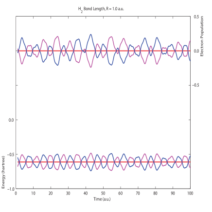
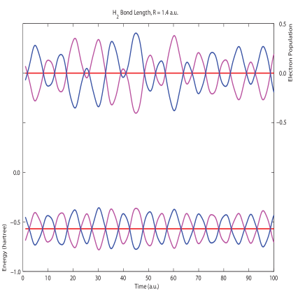
c)	d)

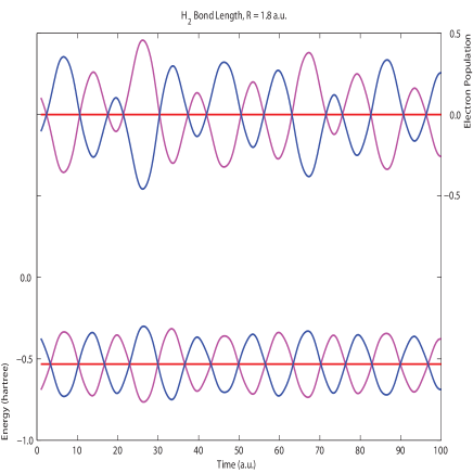
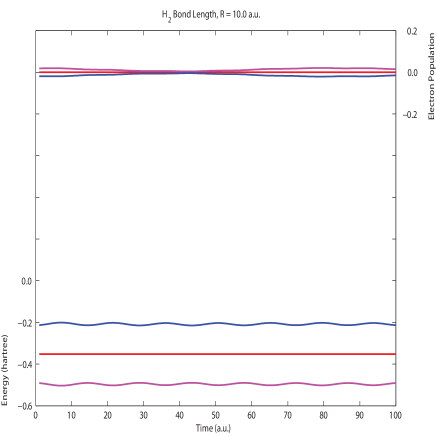
Figure 1: $H_{2}$ molecule prepared in electronic state $|1s_{A}2p_{zB}\rangle$. Coherent energy and charge transfer dynamics as function of time for bond lengths (a) $R=1.0a.u.$, (b) $R=1.4a.u.$, (c) $R=1.8a.u.$, and (d) $R=10.0a.u.$

V.1 Interacting Hydrogen Atoms

Figure 1 presents the coherent time evolution of energy and population between two interacting hydrogen atoms initially in the state $|1s_{A}2p_{Z,B}\rangle$ at various fixed internuclear separations. In each panel of the figure the curves near the top show the time evolution of the population on each hydrogen atom, together with their time average. The curves near the bottom of each panel show the time evolution of the energy of each atom, together with their time average.

The figures confirm several intuitive expectations. At large separation (Fig. 1d), when the atoms are nearly isolated, there is negligible exchange of both energy and charge. One hydrogen atom has the electronic ground state energy of $1s_{A}$, while the other hydrogen atom has the electronic excited state energy of $2p_{B}$. As the bond length shortens, with an accompanied increase in the electronic coupling strength, we observe the expected increase in the rate of energy transfer (Fig. 1(a-c)).

a)	b)
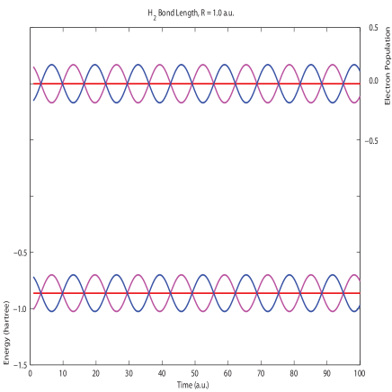
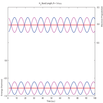
c)	d)

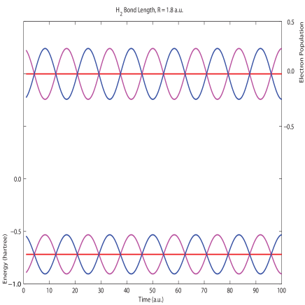
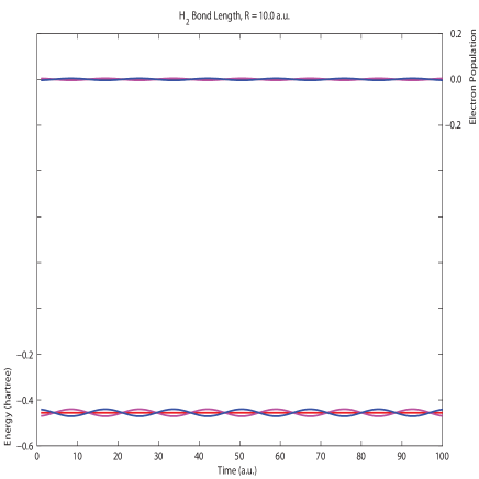
Figure 2: $H_{2}$ molecule prepared in electronic superposition state $|\Psi\rangle=1/\sqrt{2}(|\phi_{ground}\rangle+|\phi_{1^{st}excited}\rangle)\approx 1/\sqrt{2}(|\sigma_{1s}\sigma_{1s}\rangle+|\sigma_{1s}\sigma_{1s}^{*}\rangle)$. Coherent energy and charge transfer dynamics as function of time for bond lengths (a) $R=1.0a.u.$, (b) $R=1.4a.u.$, (c) $R=1.8a.u.$, and (d) $R=10.0a.u.$

The figure also reveals two interesting features. First, energy transfer is here seen to be perfectly correlated with charge transfer for all $R$. Also, the amount of energy and charge exchanged coherently between the hydrogen atoms maximizes at some intermediate separation, consistent with the fact that no energy or charge will be exchanged in the two limits, i.e., in the limit of the unified atom and that of infinitely separated atoms.

To further illustrate these patterns, consider next a hydrogen molecule prepared in a superposition of its ground and first excited electronic state (Fig. 2). The dominant contribution to the ground electronic state is from the $\sigma_{1s}^{2}$ configuration. The first excited electronic state has a primarily $\sigma_{1s}\sigma_{1s}^{*}$ character, where $\sigma_{1s}\sim(1s_{A}+1s_{B})$ is the sigma bonding molecular orbital while $\sigma^{*}_{1s}\sim(1s_{A}-1s_{B})$ is the sigma anti-bonding molecular orbital. A superposition of these states gives rise to coherent dynamics between the $1s$ orbitals on the two hydrogen atoms. Here too, the rates of charge and energy transfer as the two hydrogen atoms approach each other increase, and there is an optimal $R$ at which energy and charge transferred are maximized. At infinite separation limit the two hydrogen atoms have equal energy, corresponding to that of isolated $|1s\rangle$ hydrogen atoms.

The dynamics in this case, which involves the superposition of the two lowest singlet electronic states look much simpler than that in Fig. 1. By contrast, the state in Fig. 1 projects onto several CI eigenstates of the H₂ molecule and the dynamics therefore involves multiple timescales corresponding to many eigenenergy differences.

Decoherence

As a further example we would like to consider the effect of decoherence, e.g., decoherence induced by collisions of gaseous $H_{2}$ molecules, on the coherent energy and charge transfer dynamics. We assume that the collisions as elastic, resulting in a dephasing of otherwise coherent dynamics. Moreover, we write the complete wavefunction of our system as a product of the electronic and nuclear wavefunctions in the Born-Oppenheimer approximation. For the superposition state studied above (Fig. 2), we may write the wavefunction as:

$$|\Psi(r,R)\rangle = \frac{1}{\sqrt{2}}|\Psi_{g}(r,R)\rangle+\frac{1}{\sqrt{2}}|\Psi_{e}(r,R)\rangle$$ (48)

$$= \frac{1}{\sqrt{2}}|\psi_{g}(r;R)\rangle|\chi_{g}(R)\rangle+\frac{1}{\sqrt{2}}|\psi_{e}(r;R)\rangle|\chi_{e}(R)\rangle$$

where $|\chi_{g}(R)\rangle$ and $|\chi_{e}(R)\rangle$ are taken to be the ground vibrational wavefunctions on the respective ground and excited electronic potential energy surfaces (Fig 3). The electronic energy on hydrogen atom $A$ is then:

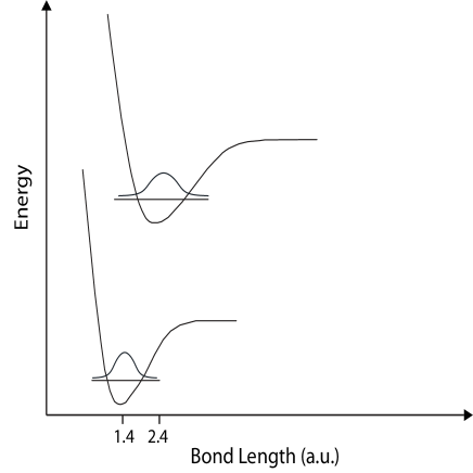
Figure 3: A sketch of the ground and excited electronic potential energy surfaces of the $H_{2}$ molecule

$$\langle E_{A}\rangle = \langle\Psi(r,R)|\mathcal{H}_{A}|\Psi(r,R)\rangle$$ (49)

$$= \frac{1}{2}\sum_{i=g,e}\int dR\chi_{i}^{*}(R)\chi_{i}(R)\left(\int dr\psi_{i}^{*}(r;R)\mathcal{H}_{A}\psi_{i}(r;R)\right)$$

$$+~{}~{}\Re\int dR\chi_{g}^{*}(R)\chi_{e}(R)\left(\int dr\psi_{g}^{*}(r;R)\mathcal{H}_{A}\psi_{e}(r;R)\right)$$

In order to make the expression more concise we define the following quantities

$$\omega_{i} = E_{i}+(n_{i}+\frac{1}{2})h\nu_{i}$$

$$\omega_{eg} = (E_{e}-E_{g})+(n_{e}+\frac{1}{2})h\nu_{e}-(n_{g}+\frac{1}{2})h\nu_{g}$$

$$E_{Ai} = \frac{1}{2}\int dR\chi_{i}^{*}(R)\chi_{i}(R)\left(\int dr\psi_{i}^{*}(r;R)\mathcal{H}_{A}\psi_{i}(r;R)\right)$$

$$\Delta_{A} = \Re\int dR\chi_{g}^{*}(R)\chi_{e}(R)\left(\int dr\psi_{g}^{*}(r;R)\mathcal{H}_{A}\psi_{e}(r;R)\right)$$ (50)

where $i=g,e$. Moreover, the time dependence of the wavefunction is easily included; only the cross term $\Delta_{A}$ will be time dependent. Thus, the time dependent energy on Hydrogen atom $A$ in the concise form

$$\begin{array}[]{lll}\langle E_{A}(t)\rangle&=&1/2\left(E_{Ag}+E_{Ae}\right)+\Delta_{A}\cos(\omega_{eg}t)\end{array}$$

The net result is a time-dependent site electronic energy, reflecting the time-dependent superposition state.

In addition, in the presence of a collisional environment the vibronic energy levels of the system are expected to fluctuate about their mean positions leading to different Hydrogen atoms in an ensemble of molecules acquiring an arbitrary phase. The expectation value of the time-dependent energy on hydrogen atom $A$ can then be expressed as

$$\begin{array}[]{lll}\overline{\langle E_{A}(t)\rangle}&=&\frac{1}{2}\left(E_{Ag}+E_{Ae}\right)+\Delta_{A}\int d\omega\cos(\omega t)f(\omega)\end{array}$$

Here $f(\omega)$ describes the distribution in energies due to environmental collisions. We assume a normal distribution of phases with mean $\omega_{eg}$. In our simulations the standard deviation is taken to be $10^{-6}$ Hartree (corresponding to a collision time on the order of 25 ps). The results of the simulation are shown in Figure 4. We observe that for the given parameters the electronic energy transfer dynamics fades out on a timescale of $4\times 10^{6}$ a.u. (100 ps).

a)	b)

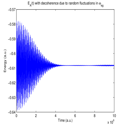
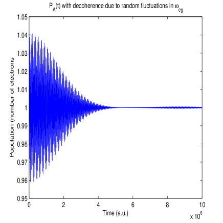
Figure 4: Decoherence induced dynamics in (a) Energy, and (b) Charge of the the $H_{2}$ molecule prepared in a superposition of the two lowest electronic states

V.2 Interacting Hydrogen Molecules

As a second example, consider the energy and population transfer dynamics between two interacting Hydrogen molecules at various separations. As an example, we fix the bond distance within each hydrogen molecule at the equilibrium bond length of $1.4a.u.$ and vary the distance between the centers of the two H₂ molecules. For each nuclear geometry the Hartree-Fock molecular orbitals of the system are determined using the 6-31G basis set, and the singlet excited states of the system are determined at the CI-Singles (CIS) level.

a)	b)
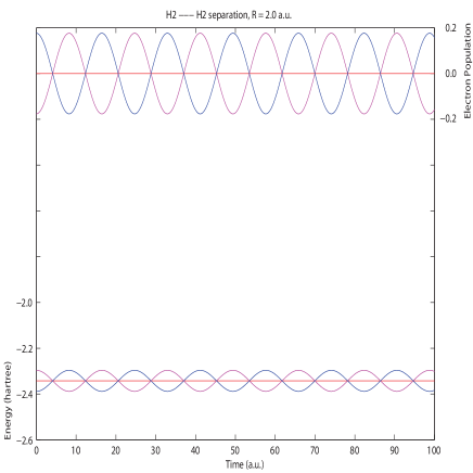
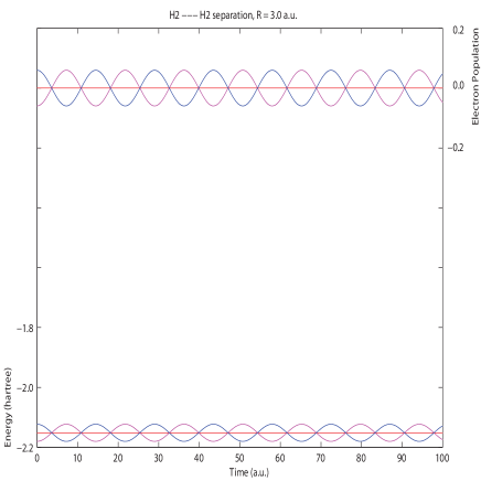
c)	d)

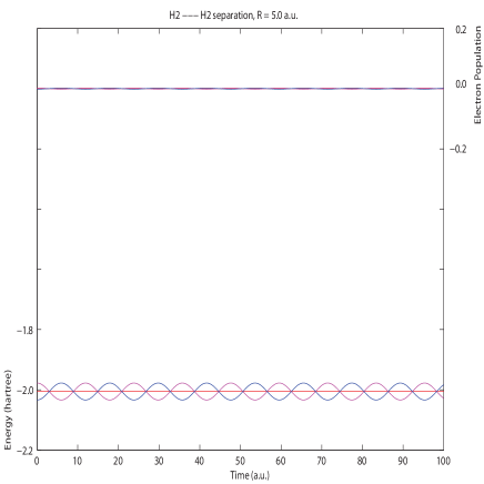
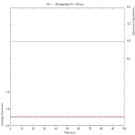
Figure 5: Interacting $H_{2}$ molecules prepared in an electronic superposition state of the ground and first excited CIS state. $|\Psi\rangle=1/\sqrt{2}(|\phi_{ground}\rangle+|\phi_{1^{st}excited}\rangle)$. Coherent energy and population transfer dynamics as function of time for bond lengths (a) $R=2.0a.u.$, (b) $R=3.0a.u.$, (c) $R=5.0a.u.$, and (d) $R=10.0a.u.$

Figure 5 presents the coherent time evolution of energy and population between the interacting molecules when the system is initiated in a superposition of its ground and first excited singlet CIS electronic state. Similarly, Figure 6 shows the dynamics for a superposition of the ground and a higher lying electronic excited state. The curves for the evolution of population and energy are respectively near the top and bottom of each panel.

The dynamics of the interacting closed shell subsystems can be compared to the dynamics of the interacting open shell system presented earlier. As before, the amplitude of population and energy exchanged between the interacting subsystems decays with increasing separation. The correlation between the population and energy dynamics within each subsystem, and the anticorrelation between the dynamics of the two subsystems also persists. However, two important differences can be discerned. First, note that charge transfer is only significant at separations below 5.0 a.u., where as significant energy transfer may persist beyond 10 a.u. This is in contrast to the two hydrogen atoms where we found that charge transfer always accompanied energy transfer. Moreover, because we no longer have the unified atom limit, the amplitude of energy and population transfer no longer shows a clear trend at small separations.

a)	b)
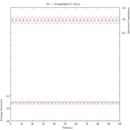
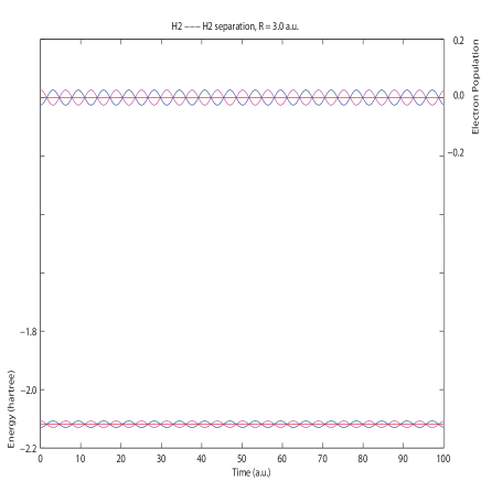
c)	d)

Figure 6: Interacting $H_{2}$ molecules prepared in an electronic superposition state of the ground and third excited CIS state. $|\Psi\rangle=1/\sqrt{2}(|\phi_{ground}\rangle+|\phi_{3^{rd}excited}\rangle)$. Coherent energy and population transfer dynamics as function of time for bond lengths (a) $R=2.0a.u.$, (b) $R=3.0a.u.$, (c) $R=5.0a.u.$, and (d) $R=10.0a.u.$

VI Summary

We have introduced a well defined operator $\mathcal{H}_{A}$ that allows, given a time dependent or time independent wavefunction $|\Psi(t)\rangle$, the computation of electronic energy on a local site in a composite molecular system, as $E_{A}=\langle\Psi(t)|\mathcal{H}_{A}|\Psi(t)\rangle$. The definition resolves numerous problems arising from electron interchange antisymmetrization that exist with naive approaches. Further, the computation of $E_{A}$, being an integral over an operator that is a function of the electronic degrees of freedom, automatically includes decoherence effects due to other degrees of freedom in the molecule. The resultant operator has been shown to give appropriate results in various limits and to provide insight into electronic energy dynamics in small molecular systems. Applications to larger systems are underway.

Acknowledgments. We acknowledge financial support of this research from the Air Force Office of Scientific Research under contract number FA9550-10-1-0260 and the Natural Sciences and Engineering Research Council of Canada. Useful discussions with Prof. G. D. Scholes during the course of this work are also gratefully acknowledged.

References

- (1) G. D. Scholes, Annu. Rev. Phys. Chem. 54, 57 (2003).
- (2) V. Sundstr om, T. Pullerits, R. van Grondelle, J. Phys. Chem. B 103, 2327 (1999).
- (3) R. van Grondelle, V. I. Novoderezhkin, Phys. Chem. Chem. Phys. 8 783 (2006).
- (4) A. Adronov, J. M. J. Fréchet, Chem. Commun. 1701 (2000).
- (5) A. Sautter, B. K. Kaletas, D. G. Schmid, R. Dobrawa, M. Zimmie, G. Jung, I. H. M. van Stokkum, L. D. Cola, R. M. Williams, F. J. Wurthner, J. Am. Chem. Soc. 127, 6719 (2005).
- (6) Y. Kobuke, Eur. J. Inorg. Chem. 2333 (2006).
- (7) G. Kodis, Y. Terazono, P. A. Liddell, J. Andreasson, V. Garg, M. Hambourger, T. A. Moore, A. L. Moore, D. Gust, J. Am. Chem. Soc. 128, 1818 (2006).
- (8) Y. Nakamura, N. Aratani, A. Osuka, Chem. Soc. Rev. 36, 831 (2007).
- (9) I. Franco and P. Brumer, J. Chem. Phys. 136, 144501 (2012); I. Franco,M. Shapiro and P. Brumer, J. Chem. Phys. 128, 244906 (2008).
- (10) H. Margenau, in Quantum Theory of Atoms, Molecules, and the Solid State, ed., P.O. Löwdin, Academic, New York (1966).
- (11) L. Li, R. G.Parr, J. Chem. Phys. 84, 1704 (1986).
- (12) A partition is “physically sound” if, given two points, and , the interaction energy between two electrons is the same whether we assume them as belonging to an atom or to a molecule li
- (13) R. McWeeny, Methods of Molecular Quantum Mechanics, 2nd Ed., Academic Press, London (2001), p.120.
- (14) N. Moiseyev, Non-Hermitian Quantum Mechanics., Cambridge University Press, New York (2011).
- (15) W. W. Parson, Modern optical spectroscopy: With examples from biophysics and biochemistry., Springer, New York (2007).
- (16) Y. R. Khan, T. E. Dykstra, G. D. Scholes, Chem. Phys. Lett. 461, 305 (2008).
- (17) Gaussian 03, Revision C.02, M. J. Frisch, et al., Gaussian, Inc., Wallingford CT, (2004).