Gravitational wave signal from massive gravity

Abstract

We discuss the detectability of gravitational waves with a time dependent mass contribution, by means of the stochastic gravitational wave observations. Such a mass term typically arises in the cosmological solutions of massive gravity theories. We conduct the analysis based on a general quadratic action, and thus the results apply universally to any massive gravity theories in which modification of general relativity appears primarily in the tensor modes. The primary manifestation of the modification in the gravitational wave spectrum is a sharp peak. The position and height of the peak carry information on the present value of the mass term, as well as the duration of the inflationary stage. We also discuss the detectability of such a gravitational wave signal using the future-planned gravitational wave observatories.

I Introduction

Since the pioneering model of massive gravity was proposed by Fierz and Pauli Fierz:1939ix , numerous attempts have been made to introduce a non-zero mass to graviton. This issue has been attracting a great deal of interest, partly because graviton mass may provide an alternative explanation for the acceleration of our universe. Namely, instead of attributing it to the existence of dark energy whose origin is still unknown, the acceleration may be simply due to modification of gravity.

Until recently, however, it has been thought that such modification by non-zero graviton mass is extremely difficult, typically leading to the emergence of ghost degrees of freedom and various pathologies. As first shown by Boulware and Deser Boulware:1973my , the source of these difficulties is associated with a helicity-$0$ mode in the gravity sector, which is absent at the quadratic order of the Fierz-Pauli massive gravity but revives at the higher order and acts as a ghost, dubbed the Boulware-Deser (BD) ghost. A remedy for this difficulty was recently proposed by Refs. deRham:2010ik ; deRham:2010kj , in which the would-be BD ghost is eliminated by adding higher-order correction terms order by order and by resumming them into a three parameter expression. Non-existence of the BD ghost in this theory was discussed and proved in Refs. Hassan:2011hr ; deRham:2011rn ; deRham:2011qq ; Hassan:2011tf ; Hassan:2011ea ; Mirbabayi:2011aa ; Golovnev:2011aa ; Kluson . Various solutions in the theory were studied in Refs. deRham:2010tw ; Koyama:2011xz ; Nieuwenhuizen:2011sq ; Koyama:2011yg ; Chamseddine:2011bu ; D'Amico:2011jj ; Gumrukcuoglu:2011ew ; Koyama:2011wx ; Comelli:2011wq ; Volkov:2011an ; vonStrauss:2011mq ; Comelli:2011zm ; Berezhiani:2011xx ; Brihaye:2011aa ; Kobayashi:2012fz . Therefore this nonlinear theory of massive gravity can be considered as a nonlinear completion of the Fierz-Pauli theory, which is the simplest and the oldest linear massive gravity theory. Having this in mind, we consider it quite natural to suppose that other massive gravity theories or, more generally, Higgs phases of gravity might find their nonlinear completions in the future.

Such examples include, but are not restricted to, ghost condensate ArkaniHamed:2003uy ; ArkaniHamed:2005gu and Lorentz-violating massive gravity theories Rubakov:2004eb ; Dubovsky:2004sg . In these examples, propagating degrees of freedom do not form a representation of $4$-dimensional Poincaré symmetry even in the exact Minkowski background. Instead, they form representations of $3$-dimensional rotational and translational symmetries. As a result, physical degrees of freedom are classified into scalar, vector and tensor parts, according to their transformation properties under the $3$-dimensional spatial rotation. Modes in different classes may behave rather differently. For instance, in the case of ghost condensate in Minkowski background, propagating degrees of freedom in the gravity sector are two tensor modes and one scalar mode. The two tensor modes behave exactly like those in general relativity (GR) while the scalar mode has an unusual dispersion relation, i.e. non-relativistic dispersion relation without a mass gap. On the other hand, in a particular class of models among those proposed in Dubovsky:2004sg , propagating degrees of freedom in the gravity sector are two tensor modes only, and their dispersion relation is massive and relativistic. From the point of view of the symmetry, i.e. $3$-dimensional spatial rotational symmetry, we expect that there should be even wider classes of models in which scalar, vector, and tensor parts behave differently.

In the present paper, for definiteness we mainly focus on a class of massive gravity models in which propagating degrees of freedom in gravity sector are only two tensor modes with a massive dispersion relation. In this case, the scalar and vector sectors behave exactly like in GR and the only modification emerges in the tensor sector: the dispersion relation of gravitational waves acquires an effective mass, which in general can be time-dependent. We shall discuss an attempt towards a nonlinear completion of such massive gravity models, but in most part of the present paper we shall consider this class of models as a purely phenomenological one to be constrained or probed by observations and experiments. We conduct the analysis based on a general quadratic action for tensor modes, and thus our results apply not only to the theories with precisely two propagating gravitational modes but also to a more general class of theories in which modification of gravity appears primarily in the tensor modes.

Being different from GR only in the tensor sector, observation of gravitational waves and/or their imprints would be the most efficient probe for the model. Therefore, in this paper we address the detectability of the effective mass of gravitational waves by means of the stochastic gravitational wave observations.

The rest of this paper is organized as follows. After describing our model in Sec. II, we discuss an attempt towards nonlinear completion of the model in Sec. III. This consideration at the very least shows that the structure of the model considered in the present paper is not forbidden by the symmetry. However, readers who are interested only in purely phenomenological aspects can safely skip Sec. III. We then derive analytic formulas for the power-spectrum of stochastic gravitational waves and discuss how to read off information about the effective mass of gravitational waves in Sec. IV. In Sec. V we show some numerical results and make comparison with the analytical results of the previous section. Sec. VI is devoted to a summary of the results and discussions.

II Model description

In the present paper we shall consider linear massive gravity models that respect the symmetry of Friedmann-Robertson-Walker (FRW) universe, i.e. the spatial homogeneity and isotropy. Metric perturbations are thus decomposed into scalar, vector and tensor parts, according to the transformation properties under the $3$-dimensional spatial rotation.

We restrict our considerations to a class of models in which the background solution is given by the ordinary FRW universe (with or without self-acceleration) and only the two tensor modes in the gravity sector are propagating on this background. For tensor-type perturbations on the FRW background, the metric can be written as

$$g_{\mu\nu}dx^{\mu}dx^{\nu}=-N(t)^{2}dt^{2}+a(t)^{2}\left[\Omega_{ij}(x^{k})+\gamma_{ij}\right]dx^{i}dx^{j},\quad\Omega_{ij}(x^{k})=\delta_{ij}+\frac{K\delta_{il}\delta_{jm}x^{l}x^{m}}{1-K\delta_{lm}x^{l}x^{m}}.$$ (1)

where $\gamma_{ij}$ is the tensor-type perturbations satisfying

$$D^{i}\gamma_{ij}=0,\quad\Omega^{ij}\gamma_{ij}=0.$$ (2)

Here, $\Omega^{ij}=(\Omega^{-1})^{ij}$, $D^{i}=\Omega^{ij}D_{j}$ and $D_{j}$ is the spatial covariant derivative compatible with the metric $\Omega_{ij}$.

By assumption, the quadratic action for the perturbation should be invariant under the spatial rotation and translation. Hence we can use the following ingredients to construct the quadratic action describing the dynamics of the tensor perturbation:

$$Ndt,\quad\sqrt{\Omega}d^{3}\vec{x},\quad\Omega_{ij},\quad D_{i},\quad\gamma_{ij},\quad\frac{1}{N}\dot{\gamma}_{ij},$$ (3)

provided that spatial indices are properly contracted to form scalar quantities. Here, $\Omega\equiv\det\Omega_{ij}$ and an overdot represents derivative with respect to the time coordinate $t$. Since the time coordinate $t$ is invariant under the spatial rotation and translation, we can also use general functions of $t$ and their derivatives.

We also demand that the action should include only up to second time derivatives of $\gamma_{ij}$ in order to avoid ghosts in the linear level and that the system respects the spatial parity invariance.

Thus, after integration by parts, one can show that the general quadratic action is of the form

$$I^{(2)}_{tensor}=\frac{M_{Pl}^{2}}{8}\int dtd^{3}x\,Na^{3}\sqrt{\Omega}\,F(t)\left[\frac{1}{N^{2}}\dot{\gamma}^{ij}\dot{\gamma}_{ij}+\gamma^{ij}\left(\sum_{n=0}^{\infty}c_{n}(t)\frac{\triangle^{n}}{a^{2n}}\right)\gamma_{ij}\right],$$ (4)

where $\gamma^{ij}\equiv\Omega^{ik}\Omega^{jl}\gamma_{kl}$, $\triangle\equiv D^{i}D_{i}$ is the Laplacian operator associated with $\Omega_{ij}$, $F(t)$ and $c_{n}(t)$ ($n=0,1,\cdots$) are general functions of the time coordinate $t$. Note that $F(t)$ must be positive definite in order to avoid appearance of ghost and strong coupling. We can then set $F(t)=1$ by a field redefinition, to be more precise, by a conformal transformation. Finally, in order to describe low energy phenomena such as cosmological evolution of gravitational waves at late time, we truncate the series expansion (the sum over $n$) at the second order spatial derivatives and obtain

$$I^{(2)}_{tensor}=\frac{M_{Pl}^{2}}{8}\int dtd^{3}x\,Na^{3}\sqrt{\Omega}\left[\frac{1}{N^{2}}\dot{\gamma}^{ij}\dot{\gamma}_{ij}+\frac{c_{g}^{2}(t)}{a^{2}}\gamma^{ij}\left(\triangle-2K\right)\gamma_{ij}-M_{GW}^{2}(t)\gamma^{ij}\gamma_{ij}\right],$$ (5)

where we have set $F=1$ by a field redefinition (or a conformal transformation) and we have defined

$$c_{g}^{2}(t)\equiv c_{1}(t),\quad M_{GW}^{2}(t)\equiv-c_{0}(t)-\frac{2Kc_{1}(t)}{a^{2}}.$$ (6)

Note that physical meaning of $c_{g}$ and $M_{GW}$ are the sound speed and effective mass of gravitational waves.

Taking advantages of the background symmetry, it is convenient to expand $\gamma_{ij}$ as

$$\gamma_{ij}=\sum_{\lambda}\int k^{2}dk\;\gamma_{k,\lambda}Y_{ij}^{\lambda}\bigl{(}\vec{k},\vec{x}\bigr{)},$$ (7)

where $k^{2}\equiv\Omega_{ij}\vec{k}^{i}\vec{k}^{j}$, $\lambda$ denotes the helicity state and $Y_{ij}^{\lambda}$ is the tensor harmonics satisfying

$$\left(\triangle+k^{2}\right)Y_{ij}^{\lambda}=0,\quad D^{i}Y_{ij}^{\lambda}=0,\quad\Omega^{ij}Y_{ij}^{\lambda}=0,\quad\int d^{3}x\sqrt{\Omega}\;\Omega^{ij}\Omega^{kl}Y_{ik}^{\lambda}\bigl{(}\vec{k},\vec{x}\bigr{)}Y_{jl}^{\lambda^{\prime}}\bigl{(}\vec{k}^{\prime},\vec{x}\bigr{)}=32\pi^{2}\delta_{\lambda\lambda^{\prime}}\delta^{3}\bigl{(}\vec{k}+\vec{k}^{\prime}\bigr{)}.$$ (8)

The equation of motion for $\gamma_{k,\lambda}$ is then

$$\bar{\gamma}_{k}^{\prime\prime}+\left(c_{g}^{2}k^{2}+a^{2}M_{GW}^{2}-\frac{a^{\prime\prime}}{a}+2Kc_{g}^{2}\right)\bar{\gamma}_{k}=0,\quad\bar{\gamma}_{k}\equiv a\gamma_{k},$$ (9)

where the prime (^′) denotes derivative with respect to the conformal time $\eta$ defined by $d\eta\equiv Ndt/a$. Since the equation of motion is identical for both polarizations, we omit the index $\lambda$ hereafter.

III Attempts toward nonlinear completion

The nonlinear theory of massive gravity recently proposed by Refs. deRham:2010ik ; deRham:2010kj eliminates the renowned BD ghost by construction and thus can be considered as a nonlinear completion of the Fierz-Pauli theory, which is the simplest and the oldest among all linear massive gravity theories. Having this in mind, we consider it quite possible that the phenomenological model described in the previous section might also find its nonlinear completions in the future.

In this section we discuss an attempt towards such a nonlinear completion. In particular, we shall derive the model with $c_{g}=1$ precisely, based on a non-trivial background in the nonlinear theory of massive gravity. Unfortunately, this construction is purely classical and fails at the quantum level DGM . Nonetheless, at the very least it shows that the structure of the model considered in the present paper, with $c_{g}=1$, is not forbidden by symmetry. Readers who are interested only in purely phenomenological aspects can safely skip this section.

The covariant action of the nonlinear massive gravity is constructed out of a $4$-dimensional metric $g_{\mu\nu}$ and four scalar fields $\varphi^{a}$ ($a=0,1,2,3$) called Stückelberg fields. The Stückelberg fields enter the action only through the tensor $f_{\mu\nu}$ defined as

$$f_{\mu\nu}=\bar{f}_{ab}(\varphi^{c})\partial_{\mu}\varphi^{a}\partial_{\nu}\varphi^{b},$$ (10)

where $\bar{f}_{ab}(\varphi^{c})$ is a non-degenerate, second-rank symmetric tensor in the field space. The spacetime metric $g_{\mu\nu}$ and the tensor $f_{\mu\nu}$ are often called physical metric and fiducial metric, respectively.

The gravity action is the sum of the Einstein-Hilbert action $I_{EH,\Lambda}$ (including a bare cosmological constant $\Lambda$) and the graviton mass term $I_{mass}$ specified below. Adding the matter action $I_{matter}$, the total action is

$$I=I_{EH,\Lambda}[g_{\mu\nu}]+I_{mass}[g_{\mu\nu},f_{\mu\nu}]+I_{matter}[g_{\mu\nu},\sigma_{I}],$$ (11)

where

$$I_{EH,\Lambda}[g_{\mu\nu}] = \frac{M_{Pl}^{2}}{2}\int d^{4}x\sqrt{-g}(R-2\Lambda),$$ (12)

$$I_{mass}[g_{\mu\nu},f_{\mu\nu}] = M_{Pl}^{2}m_{g}^{2}\int d^{4}x\sqrt{-g}\,({\cal L}_{2}+\alpha_{3}{\cal L}_{3}+\alpha_{4}{\cal L}_{4}),$$ (13)

and $\{\sigma_{I}\}$ ($I=1,2,\cdots$) represent generic matter fields. Each contribution in the mass term $I_{mass}$ is constructed as

$${\cal L}_{2} = \frac{1}{2}\left(\left[{\cal K}\right]^{2}-\left[{\cal K}^{2}\right]\right)\,,$$

$${\cal L}_{3} = \frac{1}{6}\left(\left[{\cal K}\right]^{3}-3\left[{\cal K}\right]\left[{\cal K}^{2}\right]+2\left[{\cal K}^{3}\right]\right),$$

$${\cal L}_{4} = \frac{1}{24}\left(\left[{\cal K}\right]^{4}-6\left[{\cal K}\right]^{2}\left[{\cal K}^{2}\right]+3\left[{\cal K}^{2}\right]^{2}+8\left[{\cal K}\right]\left[{\cal K}^{3}\right]-6\left[{\cal K}^{4}\right]\right)\,,$$ (14)

where the square brackets denote trace operation and

$${\cal K}^{\mu}_{\nu}=\delta^{\mu}_{\nu}-\left(\sqrt{g^{-1}f}\right)^{\mu}_{\ \nu}\,.$$ (15)

The square-root in this expression is the positive definite matrix defined through

$$\left(\sqrt{g^{-1}f}\right)^{\mu}_{\ \rho}\left(\sqrt{g^{-1}f}\right)^{\rho}_{\ \nu}=f^{\mu}_{\ \nu}\ (\equiv g^{\mu\rho}f_{\rho\nu}).$$ (16)

Note that the fiducial metric is not dynamical but fixed by the theory. In other words, the form of the fiducial metric is a part of definition of the theory. Of course, an apparent form of the fiducial metric is subject to changes under redefinition and dynamics of the Stückelberg fields. However, such changes are equivalent to coordinate transformations of the metric in the field space and thus do not change geometrical properties such as the curvature tensor in the field space. For example, if we demand the maximal symmetry, i.e. Poincaré, de Sitter or anti-de Sitter symmetry, in the field space then the fiducial metric must be Minkowski, de Sitter or anti-de Sitter metric, respectively, regardless of appearances.

In the present paper we consider a general fiducial metric of the FRW type, specified by the lapse function $n(\varphi^{0})$, the scale factor $\alpha(\varphi^{0})$ and the spacial curvature constant $K$:

$$f_{\mu\nu}=-n^{2}(\varphi^{0})\partial_{\mu}\varphi^{0}\partial_{\nu}\varphi^{0}+\alpha^{2}(\varphi^{0})\Omega_{ij}(\varphi^{k})\partial_{\mu}\varphi^{i}\partial_{\nu}\varphi^{j},\qquad\Omega_{ij}(\varphi^{k})=\delta_{ij}+\frac{K\delta_{il}\delta_{jm}\varphi^{l}\varphi^{m}}{1-K\delta_{lm}\varphi^{l}\varphi^{m}}.$$ (17)

Needless to say, this class of fiducial metrics include Minkowski, de Sitter and anti-de Sitter fiducial metrics as special cases. For example, a Minkowski fiducial metric can be rewritten as an open FRW form and allows non-trivial cosmology Gumrukcuoglu:2011ew . Note, however, that the Minkowski fiducial metric does not allow flat nor closed FRW cosmology D'Amico:2011jj . Similarly, an anti-de Sitter fiducial metric allows non-trivial open FRW cosmology but does not allow flat nor closed ones (see Appendix B). On the other hand, non-trivial open, flat, closed FRW cosmologies can be realized with a de Sitter fiducial metric (see Appendix B, and see also Ref. Gumrukcuoglu:2011zh ; Langlois:2012hk for related discussions).

In this section we consider a general FRW background plus perturbations.

$$g_{\mu\nu}=g^{(0)}_{\mu\nu}+\delta g_{\mu\nu},\qquad\varphi^{a}=x^{a}+\pi^{a}+\frac{1}{2}\pi^{b}\partial_{b}\pi^{a}+O(\epsilon^{3}),$$ (18)

where

$$g^{(0)}_{\mu\nu}dx^{\mu}dx^{\nu}=-N(t)^{2}dt^{2}+a(t)^{2}\Omega_{ij}(x^{k})dx^{i}dx^{j},\qquad\Omega_{ij}(x^{k})=\delta_{ij}+\frac{K\delta_{il}\delta_{jm}x^{l}x^{m}}{1-K\delta_{lm}x^{l}x^{m}}.$$ (19)

Here, the perturbation $\pi^{a}$ of the Stückelberg fields was defined through the exponential map, following Gumrukcuoglu:2011zh . The background equations of motion lead to

$$3H^{2}+\frac{3K}{a^{2}}=\Lambda_{\pm}+\frac{1}{M_{Pl}^{2}}\rho,\qquad-\frac{2\dot{H}}{N}+\frac{2K}{a^{2}}=\frac{1}{M_{Pl}^{2}}\left(\rho+P\right),\qquad\frac{\alpha(t)}{a(t)}=X_{\pm},$$ (20)

where a dot represents derivative with respect to $t$, $H\equiv\dot{a}/(Na)$ is the Hubble expansion rate of the background physical metric, $\rho$ and $P$ are the matter energy density and pressure, and

$$X_{\pm}\equiv\frac{1+2\alpha_{3}+\alpha_{4}\pm\sqrt{1+\alpha_{3}+\alpha_{3}^{2}-\alpha_{4}}}{\alpha_{3}+\alpha_{4}},\qquad\Lambda_{\pm}=-m_{g}^{2}(1-X_{\pm})[3-X_{\pm}+\alpha_{3}(1-X_{\pm})].$$ (21)

(See Ref. Gumrukcuoglu:2011zh or Appendix B for derivation.) Note that the background physical metric follows the Friedmann equation with an effective cosmological constant $\Lambda_{\pm}$ and thus the universe exhibits self-acceleration if $\Lambda_{\pm}>0$.

Thanks to the exponential map used to define $\pi^{a}$ in (18), the action for cosmological perturbations around the self-accelerating FRW background manifestly respects the background symmetry. This allows us to decompose the perturbations into scalar, vector and tensor parts, according to transformation properties under spatial diffeomorphism. A priori, because of the inclusion of four Stückelberg fields, we might expect cosmological perturbations in the gravity sector to consist of $6$ degrees of freedom: $2$ tensor, $2$ vector and $2$ scalar modes. Actually, since the theory is constructed in such a way that the would-be BD ghost is completely excised, one would instead expect that cosmological perturbations in the gravity sector should consist of $5$ degrees of freedom: $2$ tensor, $2$ vector and $1$ scalar modes. Surprisingly enough, the gauge-invariant analysis of the quadratic action in Gumrukcuoglu:2011zh has shown that the scalar and vector degrees have vanishing kinetic terms. Assuming these degrees are non-dynamical, we may integrate them out, then find that in the scalar and vector sectors, gauge-invariant variables constructed from metric and matter perturbations have exactly the same quadratic action as in general relativity.

Hence, for linear perturbations around the self-accelerating FRW background, difference from general relativity arises only in the tensor sector. Assuming that there is no tensor-type contribution from matter fields $\sigma_{I}$ for simplicity, the quadratic action for the tensor sector is given by (5) with

$$c_{g}=1,\quad M_{GW}^{2}=\pm(r-1)m_{g}^{2}X_{\pm}\sqrt{1+\alpha_{3}+\alpha_{3}^{2}-\alpha_{4}},\quad r=\frac{H}{X_{\pm}H_{f}}.$$ (22)

Here, $H\equiv\dot{a}/(Na)$ and $H_{f}\equiv\dot{\alpha}/(n\alpha)$ are Hubble expansion rates of the background physical metric and the fiducial metric, respectively. Note that $r$ and thus $M_{GW}$ are time-dependent functions determined by the ratio $H/H_{f}$.

We have derived the model described in the previous section with $c_{g}=1$. As already stated, the derivation is purely classical and fails at the quantum level DGM . For this reason we do not consider this construction as a realistic one. Nonetheless, at the very least this shows that the structure of the model is not forbidden by symmetry. It may be worthwhile focusing on different models such as Refs. Dubovsky:2004sg ; Blas:2009my ; deRham:2012kf and/or investigating cosmological perturbations around new classes of cosmological backgrounds such as those found in Ref. Koyama:2011wx ; Kobayashi:2012fz ; Gumrukcuoglu:2012aa ; Motohashi:2012jd , towards a successful nonlinear completion.

For example, in one of Lorentz-violating massive gravity theories Dubovsky:2004sg , the symmetry $\phi^{i}\to\phi^{i}+\xi^{i}(\phi^{0})$ ensures the existence of three instantaneous modes in a fully nonlinear level, where $\xi^{i}$ ($i=1,2,3$) are arbitrary functions of $\phi^{0}$. Invoking the additional scaling symmetry $\phi^{0}\to\lambda\phi^{0}$, $\phi^{i}\to\lambda^{-\gamma}\phi^{i}$, and setting the $3$-dimensional fiducial metric to be flat, one can show that linear perturbations around a flat FRW background include only three physical modes in the gravity sector (except for the three instantaneous modes): two tensor modes representing massive gravitons and one scalar mode stemmed from $\phi^{0}$ Dubovsky:2005dw . The scalar mode is analogous to the ghost condensate ArkaniHamed:2003uy ; ArkaniHamed:2005gu in the sense that it is massless and has vanishing sound speed. Since the modification of gravity due to ghost condensate is rather mild , this setup may be considered as a good candidate for nonlinear completion. However, in the ghost condensate, because of the vanishing sound speed, the leading gradient terms come from higher derivative terms and thus the inclusion of higher derivative terms is essential for the stability of the system at (relatively) short distances. When the above mentioned scaling symmetry is imposed, this implies that higher derivative terms must be introduced not only for $\phi^{0}$ but also for $\phi^{i}$. It is important that those higher derivative terms for $\phi^{i}$ can in principle introduce tiny time kinetic terms but that they do not lead to strongly coupled (and possibly ghosty) new degrees of freedom in the regime of validity of the effective field theory, even in curved backgrounds away from the decoupling limit. To see this, note that the existence of instantaneous modes implies that such a time kinetic term, if exists, should have spatial derivatives acted on it. Therefore, as far as those time kinetic terms are suppressed by the cutoff scale of the theory, the corresponding would-be new degrees of freedom have frequencies above the cutoff. For this reason, it is expected that higher derivative terms do not introduce any dangerous new degrees of freedom. It is certainly worthwhile investigating this in concrete setups. Detailed analysis of these issues is beyond the scope of the present paper and thus we leave it for the future.

IV Stochastic gravitational wave spectrum

To clarify the influence of $M_{GW}$ on the observable quantities, we seek approximate solutions to Eq. (9) for a generic $M_{GW}(t)$, by considering super-horizon modes to be frozen and sub-horizon modes to follow the WKB-type evolution. We then derive approximate analytic formulas for the energy and power spectra. For simplicity we set

$$c_{g}=1,$$ (23)

throughout this and the forthcoming sections except for Sec. IV.5.4, where we give a brief comment on the case of a general $c_{g}$.

IV.1 Horizon re-entry

¿From the action (5) and the equation of motion (9) with $c_{g}=1$, one can easily read off the dispersion relation as

$$\omega^{2}=\frac{k^{2}}{a^{2}}+M_{GW}^{2},$$ (24)

where $\omega$ is the effective frequency with respect to the proper time $\tau$ defined by $d\tau=Ndt=ad\eta$. Here, since the comoving momentum $k$ appears only through the combination $\sqrt{k^{2}+2K}$, we have renamed this combination as $k$ so that $K$ does not appear explicitly. We shall still call $k$ (after this redefinition) comoving momentum. To consider the case that the graviton mass becomes in effect in the evolution history and also to simplify the analysis, we assume that the mass squared $M_{GW}^{2}$, which is an arbitrary function given by Eq. (6), dominates the right hand side of (24) at late time and that it does not lead to instability, i.e.

$$\partial_{t}(a^{2}M_{GW}^{2})>0,\quad M_{GW}^{2}>0.$$ (25)

(See Sec. V and Appendix B for a simple example in which these conditions actually hold.)

The frequency $\omega$ given by the dispersion relation (24) is relevant and the tensor mode oscillates with this frequency if and only if it is sufficiently high compared with the cosmic expansion, i.e. $\omega^{2}\gg H^{2}$. On the other hand, when $\omega^{2}\ll H^{2}$, the equation of motion (9) allows a growing solution $\bar{\gamma}_{k}\propto a$ and thus $\gamma_{k}\simeq const$. At a given moment of time, a mode with $\omega^{2}\gg H^{2}$ is called sub-horizon and a mode with $\omega^{2}\ll H^{2}$ is called super-horizon, as usual. For a given mode with comoving momentum $k$, the time when $\omega^{2}\simeq H^{2}$ is called horizon crossing, again, as usual.

We suppose that scale-invariant super-horizon gravitational waves are generated in the early universe, e.g. through inflation. In the present paper we concentrate on the subsequent evolution of gravitational waves, assuming for simplicity that the matter energy density and pressure in the background equation of motion (20) satisfy the strong energy condition ($\rho+3P>0$). With this assumption, $a^{2}\rho$ decreases as the universe expands. Since the curvature term ($3K/a^{2}$) is small (less than a few percent of $3H^{2}$) at present time, this implies that the curvature term is negligible throughout the evolution. Hence, before the effective cosmological constant $\Lambda_{\pm}$ starts dominating the universe, $a^{2}H^{2}$ decreases as the universe expands and, under the assumption (25), super-horizon modes generated in the early universe eventually cross the horizon and become sub-horizon. This type of horizon crossing is called horizon re-entry, as usual.

For a mode with comoving momentum $k$, the time of horizon re-entry is denoted as $t=t_{k}$ and defined as the solution to

$$\omega^{2}(t_{k})=H^{2}(t_{k}).$$ (26)

We denote the values of $a$ and $H$ at $t=t_{k}$ as $a_{k}$ and $H_{k}$, respectively. For comparison, we define the time of horizon re-entry in the massless case (GR) $t_{k}^{GR}$ by

$$\frac{k^{2}}{a^{2}}=H^{2}\quad\mbox{at}\quad t=t_{k}^{GR},$$ (27)

and denote the values of $a$ and $H$ at $t=t_{k}^{GR}$ as $a_{k}^{GR}$ and $H_{k}^{GR}$, respectively.

IV.2 Classification of modes

As defined above, the modes re-enter the horizon when the effective frequency $\omega$ given by (24) exceeds the Hubble expansion rate $H$. Thus, the discussion of the evolution of the modes can be reduced to the determination of the time when either the mass contribution $a\,M_{GW}$ or the comoving momentum $k$ exceeds the comoving horizon scale $a\,H$. Hence, in this subsection, we discuss the evolution of $a\,M_{GW}$ and $a\,H$ relative to $k$.

We define two special scales which characterize classification of the different modes. First, we introduce the critical momentum $k_{c}$ for which, the horizon crossing occurs at time $t=t_{c}$, when both the momentum and the mass term contribute equally to the frequency,

$$k_{c}=a_{c}M_{GW}(t_{c})=a_{c}H_{c}/\sqrt{2}\,,$$ (28)

where $a_{c}\equiv a(t_{c})$ and $H_{c}\equiv H(t_{c})$. After the time $t_{c}$, the sub-horizon evolution of a mode with $k<k_{c}$ is completely determined by the mass term. The second scale we define is

$$k_{0}\equiv a_{0}\,M_{GW}(t_{0})\,,$$ (29)

that characterizes the momentum of the mode for which, the mass term starts to dominate from today on, $t>t_{0}$. If $k_{c}<k_{0}$ (or equivalently, by Eq. (25), $t_{c}<t_{0}$), then the modes which are affected by the mass term will be within the observable universe today. In Fig. 1, we show the characteristic momenta $k_{c}$ and $k_{0}$ in relation to the evolution.

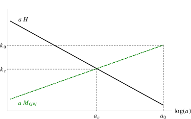
Figure 1: Schematic plot for the evolution of $a\,M_{GW}$ and $a\,H$. We show the critical momentum $k_{c}$, defined in (28), for which, the mass and momentum contributions are equal at the time of re-entry, while $k_{0}$, defined in (29), is the momentum of the mode for which the mass term became important just today.

Throughout this paper we assume that

$$k_{c}<k_{0},\quad a_{c}<a_{0}.$$ (30)

If $a_{c}<a_{0}$ is not satisfied, the effective mass would always be smaller than the Hubble expansion rate all the way down to the present time, and would never affect cosmological evolution of gravitational waves. We also assumed $k_{c}<k_{0}$ for simplicity.

With these considerations, we classify the modes depending on their momenta:

• Short wavelength ($k_{0}<k$): modes for which the momentum is large enough to dominate the frequency after horizon re-entry. We thus have $t_{k}\simeq t_{k}^{GR}$, $a_{k}\simeq a_{k}^{GR}$ and $H_{k}\simeq H_{k}^{GR}$. Since the mass term never becomes important, the evolution is indistinguishable from its counterpart in GR.

• Intermediate wavelength ($k_{c}<k<k_{0}$): modes for which the mass term becomes dominant after horizon re-entry, but before today. We still have $t_{k}\simeq t_{k}^{GR}$, $a_{k}\simeq a_{k}^{GR}$ and $H_{k}\simeq H_{k}^{GR}$. We expect slight modifications with respect to GR signal.

• Long wavelength ($k<k_{c}$): modes for which the mass term is dominant at horizon re-entry. Since the momentum is negligible throughout the evolution after horizon exit, their evolution is the same, regardless of their momenta. In other words, $t_{k}$ for these modes is roughly independent of the momentum and all modes of this type re-enter the horizon simultaneously. We thus have $t_{k}\simeq t_{c}$, $a_{k}\simeq a_{c}$ and $H_{k}\simeq H_{c}$. The largest deviation from general relativity is expected in this category.

This classification is summarized in Fig. 2.

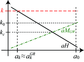
(a) Short wavelength: $k_{0}<k$

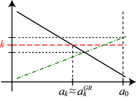
(b) Intermediate wavelength: $k_{c}<k<k_{0}$

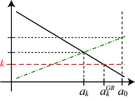
(c) Long wavelength: $k<k_{c}$

Figure 2: Examples for each type of momenta based on the classification in the main text. For modes with short and intermediate wavelengths ($k_{0}<k$ and $k_{c}<k<k_{0}$), the horizon entry time is the same as in GR, with $a_{k}\sim a_{k}^{GR}$. However, for modes with long wavelength ($k<k_{c}$), the momentum term never becomes dominant and the horizon entry in the massive theory occurs earlier than in GR, i.e. $a_{k}<a_{k}^{GR}$.

In the forthcoming calculations, especially in subsection IV.5, we will need an explicit expression for $a_{k}^{GR}$. In order to determine this expression, we use the Friedmann equation for a composite fluid with nonrelativistic matter and radiation, that is,

$$H=\frac{H_{eq}}{\sqrt{2}}\,\left(\frac{a_{eq}}{a}\right)^{2}\,\sqrt{1+\frac{a}{a_{eq}}}\,,$$ (31)

where the subscript “eq” denotes the time of matter–radiation equality. (See footnote 3.) Then, the horizon crossing time in GR can be found by solving

$$k^{2}=\frac{H_{eq}^{2}\,a_{eq}^{4}}{2\,(a_{k}^{GR})^{2}}\,\left(1+\frac{a_{k}^{GR}}{a_{eq}}\right)\,.$$ (32)

Depending on the dominant fluid at $t=t_{k}^{GR}$, the scale factor $a_{k}^{GR}$ will have a different momentum dependence,

$$\frac{a_{k}^{GR}}{a_{eq}}=\left\{\begin{array}[]{lll}\frac{k_{eq}^{GR}}{\sqrt{2}\,k}&\quad\mbox{for}&k\gg k_{eq}\\ \left(\frac{k_{eq}^{GR}}{\sqrt{2}\,k}\right)^{2}&\quad\mbox{for}&k\ll k_{eq}\end{array}\right.\,,$$ (33)

where $k_{eq}^{GR}\equiv a_{eq}H_{eq}$ is the comoving momentum of the mode which crosses the horizon at the time of equality, in GR.

IV.3 WKB solution

As already stated in subsection IV.1, a super-horizon mode stays constant and, thus, its absolute value is given by

$$|\gamma_{k}|=A(k)\,,\quad{\rm for~{}}t<t_{k}\,,$$ (34)

where $A(k)$ is the amplitude of the mode at the time of its generation, and for slow-roll inflation, is given by

$$A(k)=\frac{H_{*}}{M_{Pl}\,k^{3/2}}\,.$$ (35)

Here, $H_{*}$ is the value of the Hubble expansion rate at the time of horizon exit during inflation.

Once the mode re-enters the horizon at time $t=t_{k}$, it starts to oscillate with frequency $\omega$. Assuming that the evolution of the frequency is adiabatic, i.e. $\omega^{2}\gg H^{2}$, we can use the WKB approximation to obtain the solution

$$\gamma_{k}(t)=\frac{C(k)}{\,\sqrt{\omega(t)a^{3}(t)}}\,\exp\left(-i\,\int\omega\,a\,d\eta\right)\,,\quad{\rm for~{}}t>t_{k}\,,$$ (36)

where $C(k)$ is a $k$-dependent integration constant. By using the thin-horizon approximation, with which we suppose the mode re-enters the horizon sufficiently fast, we can match the super-horizon frozen solution (34) and the sub-horizon oscillating solution (36) at $t=t_{k}$, resulting in

$$\frac{|\gamma_{k}(t)|}{A(k)}=\sqrt{\frac{\omega_{k}}{\omega(t)}\frac{a_{k}^{3}}{a^{3}(t)}}\,,\quad{\rm for~{}}t>t_{k}\,,$$ (37)

where $\omega_{k}\equiv\omega(t_{k})=H_{k}$.

For comparison, the corresponding solution in the massless case (GR) is obtained by simply replacing $\omega\to k/a$ and $t_{k}\to t_{k}^{GR}$ as

$$\frac{|\gamma_{k}^{GR}(t)|}{A(k)}=\frac{a_{k}^{GR}}{a(t)}\,,\quad{\rm for~{}}t>t_{k}^{GR}\,.$$ (38)

IV.4 Power spectrum

Observationally speaking, what we are interested in is the amplitude of sub-horizon gravitational waves today as a function of frequency. We thus would like to compare the amplitude of sub-horizon gravitational waves in massive gravity with that in GR at the same frequency today. For this purpose we define the power spectrum of sub-horizon gravitational waves as

$${\cal P}(\omega_{0})\equiv\left.\frac{d}{d\ln\omega_{0}}\langle\gamma_{ij}\gamma^{ij}\rangle\right|_{t=t_{0}}=\frac{\omega_{0}^{2}}{\omega_{0}^{2}-M_{GW,0}^{2}}\frac{2k^{3}}{\pi^{2}}\left|\gamma_{k}(t_{0})\right|^{2},\quad k=a_{0}\sqrt{\omega_{0}^{2}-M_{GW,0}^{2}}~{},$$ (39)

where

$$\omega_{0}=\omega(t_{0}),\quad M_{GW,0}=M_{GW}(t_{0}),$$ (40)

and we have used

$$\frac{d\ln k}{d\ln\omega_{0}}=\frac{\omega_{0}^{2}}{\omega_{0}^{2}-M_{GW,0}^{2}}.$$ (41)

The power spectrum in GR with the same frequency is

$${\cal P}_{GR}(\omega_{0})=\frac{2k^{\prime 3}}{\pi^{2}}\left|\gamma_{k^{\prime}}^{GR}(t_{0})\right|^{2},\quad k^{\prime}=a_{0}\omega_{0}\,,$$ (42)

where $k^{\prime}$ corresponds to the momentum of the mode in GR with frequency $\omega_{0}$.

By using the WKB solution given in the previous subsection, we obtain

$${\cal P}(\omega_{0})=\left(\frac{k^{\prime}a_{k}}{ka_{0}}\right)^{2}\frac{\omega_{k}a_{k}}{\omega_{0}a_{0}}\,{\cal P}_{prim}(k),$$ (43)

and

$${\cal P}_{GR}(\omega_{0})=\left(\frac{a_{k^{\prime}}^{GR}}{a_{0}}\right)^{2}{\cal P}_{prim}(k^{\prime}),$$ (44)

where we have defined the primordial power spectrum by

$${\cal P}_{prim}(k)\equiv\frac{2k^{3}}{\pi^{2}}A^{2}(k).$$ (45)

IV.5 Enhancement of gravitational waves and cutoff

We are interested in the ratio of the power spectrum in massive gravity to that in GR at the same frequency today $\omega_{0}$. From the results in the previous subsection, we obtain

$$\frac{{\cal P}(\omega_{0})}{{\cal P}_{GR}(\omega_{0})}=\frac{{\cal P}_{prim}(k)}{{\cal P}_{prim}(k^{\prime})}{\cal S}^{2}(\omega_{0}),$$ (46)

where

$${\cal S}(\omega_{0})=\frac{k^{\prime}a_{k}}{k\,a_{k^{\prime}}^{GR}}\sqrt{\frac{\omega_{k}a_{k}}{\omega_{0}a_{0}}},\quad k=a_{0}\sqrt{\omega_{0}^{2}-M_{GW,0}^{2}},\quad k^{\prime}=a_{0}\omega_{0}.$$ (47)

In the rest of this subsection, we estimate the enhancement factor ${\cal S}(\omega_{0})$ for the three classes of modes introduced in subsection IV.2.

IV.5.1 Short wavelength modes: $k_{0}\ll k$

For these small-scale gravitational waves, the frequency $\omega$ defined by (24) is dominated by the momentum throughout the evolution, i.e. $\omega\simeq k/a$. Thus we have

$$\omega_{k}\simeq\frac{k}{a_{k}},\quad\omega_{0}\simeq\frac{k}{a_{0}},\quad k^{\prime}\simeq k.$$ (48)

Also, as illustrated in Fig. 2(a), the horizon re-entry occurs at the same time as in the GR analogue,

$$a_{k}\simeq a_{k}^{GR}\simeq a_{k^{\prime}}^{GR}.$$ (49)

Thus, this case does not give rise to an enhancement:

$${\cal S}(\omega_{0})\simeq 1.$$ (50)

IV.5.2 Intermediate wavelength modes: $k_{c}\ll k\ll k_{0}$

For the intermediate-scale gravitational waves, frequency at the time of horizon re-entry is dominated by momentum,

$$\omega_{k}\simeq\frac{k}{a_{k}}\,,$$ (51)

giving rise to the same re-entry time as in GR

$$a_{k}\simeq a_{k}^{GR}.$$ (52)

On the other hand, the mass term comes to dominate at later time, yielding for the frequency of the modes today

$$\omega_{0}\simeq M_{GW,0}=\frac{k_{0}}{a_{0}},\quad k^{\prime}\simeq k_{0}.$$ (53)

Thus, these modes will undergo an enhancement:

$${\cal S}(\omega_{0})\simeq\frac{a_{k}^{GR}}{a_{k_{0}}^{GR}}\sqrt{\frac{k_{0}}{k}}.$$ (54)

By using the formula (33), we obtain

$${\cal S}(\omega_{0})\simeq\left\{\begin{array}[]{lll}\sqrt{\frac{k_{0}^{3}}{k^{3}}}\simeq\left(\frac{\omega_{0}^{2}}{M_{GW,0}^{2}}-1\right)^{-3/4}&\quad\mbox{for}&k_{eq}\ll k\ll k_{0}\\ \sqrt{\frac{k_{eq}^{2}k_{0}^{3}}{2k^{5}}}\simeq\frac{k_{eq}}{\sqrt{2}k_{0}}\left(\frac{\omega_{0}^{2}}{M_{GW,0}^{2}}-1\right)^{-5/4}&\quad\mbox{for}&k\ll k_{eq}\ll k_{0}\\ \sqrt{\frac{k_{0}^{5}}{k^{5}}}\simeq\left(\frac{\omega_{0}^{2}}{M_{GW,0}^{2}}-1\right)^{-5/4}&\quad\mbox{for}&k\ll k_{0}\ll k_{eq}\end{array}\right.\,.$$ (55)

IV.5.3 Long wavelength modes: $k\ll k_{c}$

When these modes re-enter the horizon, the mass term is already dominant in their frequency

$$\omega_{k}\simeq M_{GW}(t_{k}),$$ (56)

and thus the re-entry time is independent of the comoving momentum. In other words, all modes with $k\ll k_{c}$ re-enter the horizon simultaneously when the Hubble expansion rate and the effective mass of gravitational waves agree

$$H(t_{k})\simeq M_{GW}(t_{k}).$$ (57)

Up to factors of order one, this is essentially the definition of $t_{c}$ introduced in subsection IV.2 and thus $t_{k}\simeq t_{c}$. Hence, we have

$$a_{k}\simeq a_{c},\quad\omega_{c}\simeq M_{GW}(t_{c})=\frac{k_{c}}{a_{c}}.$$ (58)

Since we have assumed that $aM_{GW}$ is a growing function of time, $M_{GW}$ dominates $\omega$ at $t=t_{0}$ as well:

$$\omega_{0}\simeq M_{GW,0}=\frac{k_{0}}{a_{0}},\quad k^{\prime}\simeq k_{0}.$$ (59)

Thus we obtain

$${\cal S}(\omega_{0})\simeq\frac{a_{c}}{a_{k_{0}}^{GR}}\frac{\sqrt{k_{0}k_{c}}}{k}\simeq\frac{a_{c}}{a_{k_{0}}^{GR}}\sqrt{\frac{k_{c}}{k_{0}}}\left(\frac{\omega_{0}^{2}}{M_{GW,0}^{2}}-1\right)^{-1/2}.$$ (60)

IV.5.4 Summary of enhancement factor

As one can see from the schematic plot in Fig. 3, qualitative behavior of the amplification factor ${\cal S}(\omega_{0})$ is summarized as follows.

• No modification in the high frequency range ($k_{0}<k\,\Leftrightarrow\,\sqrt{2}M_{GW,0}<\omega_{0}$): ${\cal S}(\omega_{0})$ stays almost unity.

• Modest enhancement in the intermediate frequency range ($k_{c}<k<k_{0}\,\Leftrightarrow\,\omega_{c}<\omega_{0}<\sqrt{2}M_{GW,0}$): ${\cal S}(\omega_{0})$ is proportional to some positive powers of $(\omega_{0}^{2}-M_{GW,0}^{2})^{-1}$ as shown in Eq. (55), and thus increases as $\omega_{0}$ decreases.

• Sharp peak just above the cutoff ($0<k<k_{c}\,\Leftrightarrow\,M_{GW,0}<\omega_{0}<\omega_{c}$): ${\cal S}(\omega_{0})$ is proportional to $(\omega_{0}^{2}-M_{GW,0}^{2})^{-1/2}$, and thus it diverges in the limit $\omega_{0}\to M_{GW,0}$.

• No signal below the cutoff ($\omega_{0}<M_{GW,0}$): ${\cal S}(\omega_{0})=0$.

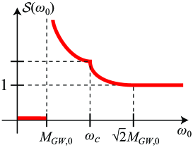
Figure 3: Schematic plot of the amplification factor ${\cal S}(\omega_{0})$.

We emphasize that the qualitative feature of the spectrum shown in Fig. 3 is quite universal; as long as $a\,M_{GW}$ is an increasing function of time and the two scales $k_{c}<k_{0}$ are well separated, it applies to any fiducial metric, or even other models of massive gravity.

Before going into the next subsection, we briefly comment on the case where $c_{g}$ is not constant. We assume that $c_{g}k/a$ becomes equal to each of $H$ and $M_{GW}$ only once, similarly to the case of constant $c_{g}$ we have discussed. In this case, Eqs. (24) are altered into (28) and (29) into

$$\omega^{2}=\frac{c_{g}(t)k^{2}}{a^{2}}+M_{GW}^{2},\qquad c_{g}(t_{c})k_{c}=a_{c}M_{GW}(t_{c})=a_{c}H_{c},\qquad c_{g}(t_{0})k_{0}=a_{0}M_{GW}(t_{0}).$$ (61)

We redefine the horizon crossing time $t_{k}$ using $\omega$ in this equation. Using these new definitions, we may repeat the derivations in the previous subsections to obtain the formula for ${\cal S}(\omega_{0})$. Its expression is given by

$${\cal S}(\omega_{0})=\frac{k^{\prime}a_{k}}{c_{g}(t_{0})k\,a_{k^{\prime}}^{GR}}\sqrt{\frac{\omega_{k}a_{k}}{\omega_{0}a_{0}}}\simeq\begin{cases}\frac{a_{k}}{a^{GR}_{c_{g}(t_{0})k}}\sqrt{\frac{c_{g}(t_{k})}{c_{g}(t_{0})}}&(k_{0}\ll k)\\ \frac{a_{k}}{a^{GR}_{c_{g}(t_{0})k_{0}}}\sqrt{\frac{c_{g}(t_{k})k_{0}}{c_{g}(t_{0})k}}&(k_{c}\ll k\ll k_{0})\\ \frac{a_{c}}{a^{GR}_{c_{g}(t_{0})k}}\sqrt{\frac{c_{g}(t_{c})k_{0}k_{c}}{c_{g}(t_{0})k^{2}}}&(k\ll k_{c})\end{cases}~{}.$$ (62)

Note that also the primordial spectrum ${\cal P}_{prim}(k)$ may be shifted if $c_{g}(t)$ is shifted from the unity in the inflationary era.

IV.6 Signatures in the spectrum

In the previous subsection, we have shown that the enhancement factor ${\cal S}(\omega_{0})$ defined by (46) diverges in the limit $\omega_{0}\to M_{GW,0}+0$. However, the power spectrum ${\cal P}(\omega_{0})$ itself does not diverge, provided that

$$\lim_{k\to+0}k^{-2}{\cal P}_{prim}(k)<\infty.$$ (63)

This is the case, for example, if the primordial gravitational waves are generated by inflation in the early universe and if the e-folding number of the inflation is finite. Nonetheless, from the divergence of ${\cal S}(\omega_{0})$ it is likely that the power spectrum ${\cal P}(\omega_{0})$ has a sharp peak just above the cutoff at $\omega_{0}=M_{GW,0}$. Below the cutoff, the power spectrum should vanish.

The peak just above $\omega_{0}=M_{GW,0}$ may become rather high if the primordial spectrum ${\cal P}_{prim}(k)$ of gravitational waves continues to a far infrared. For example, this situation can be realized when the duration of inflation is prolonged. Concretely, ${\cal P}_{prim}(k)$ is expected to continue down to $k\sim a_{0}H_{0}e^{-N_{extra}}$, where $N_{extra}$ is the number of additional e-folds to the minimum needed for the spatial curvature to stay below the observational bounds. Hence, by the formula (60), the enhancement factor at the peak is estimated as

$${\cal S}_{peak}\sim\frac{a_{c}}{a_{k_{0}}^{GR}}\frac{\sqrt{k_{0}k_{c}}}{a_{0}H_{0}}e^{N_{extra}}.$$ (64)

Future observation of gravitational waves may reveal deviation from the spectrum predicted by GR. If the cutoff and the sharp peak just above it are found, then this might be a signature of massive gravity. In this case, from the frequency at the cutoff one can read off the value of $M_{GW,0}$. It might also be possible to read off some information about the fall-off behavior of the primordial spectrum in the far infrared (63), from the height of the peak.

V Numerical results

In the previous section we have shown that the power spectrum of stochastic gravitational waves in massive gravity vanishes at frequencies below a cutoff and a sharp peak is expected just above the cutoff. The cutoff frequency agrees with the effective mass of gravitational waves today $M_{GW,0}$. It is therefore interesting if the effective mass $M_{GW,0}$ is within the frequency range to which gravitational wave detectors are sensitive. For example, evolved Laser Interferometer Space Antenna (eLISA) AmaroSeoane:2012km is sensitive to the frequency range $10^{-4}-1$ Hz and aims to be sensitive for $3\times 10^{-5}-1$ Hz. For lower frequencies, pulsar timing arrays such as the Square Kilometre Array (SKA) SKA and the Parkes Pulsar Timing Array (PPTA) PPTA have sensitivities down to $10^{-8}$ Hz. The combined sensitivity range for these observatories is thus $10^{-8}-1$ Hz. Taking into account the bound $M_{GW,0}\lesssim 10^{-5}\,\text{Hz}$ from the orbital decays of binary pulsars Finn:2001qi , one might be able to hope future detection of the cutoff and the peak in the gravitational wave spectrum if

$$10^{-8}\,\text{Hz}\lesssim M_{GW,0}\lesssim 10^{-5}\,\text{Hz}.$$ (65)

The spectrum obtained analytically in the previous section, especially its peak structure, is not sensitive to the history of $M_{GW}(t)$ in the early universe but is essentially determined by its present value $M_{GW,0}$. Thus, for the purpose of numerical calculations, we consider time-independent $M_{GW}=M_{GW,0}$ in the range (65).

In Fig. 4, we compare the numerically obtained gravitational wave spectrum and the analytic estimation derived in the previous section. The former is obtained by numerically solving Eq. (9) with the mass term assumed to be $M_{GW,0}=10^{10}H_{0}\sim 2\times 10^{-7}\,\text{Hz}$, for which we find $k_{0}/H_{0}=10^{10}$ and $k_{c}/H_{0}\sim 10^{4}$. The evolution of the gravitational wave inside the Hubble or mass horizon is calculated using the WKB solution, Eq. (36), in order to save computational time. The latter is obtained by multiplying the numerically obtained spectrum in GR by the analytically obtained factor ${\cal S}(\omega_{0})$, given in Eq. (62). In both cases, we assume that the evolution of the Hubble expansion rate is determined by the density parameters of radiation $\Omega_{r}h^{2}=4.15\times 10^{-5}$, matter $\Omega_{m}h^{2}=0.1344$, and cosmological constant (either the genuine cosmological constant or the effective one induced by the graviton mass term, or their sum) $\Omega_{\Lambda}=0.734$, with the normalized Hubble rate $h=0.71$ Komatsu:2010fb . The primordial spectrum is assumed to be scale-invariant and its amplitude is normalized by ${\cal P}_{\text{prim}}(k)=2.43\times 10^{-10}$, where we assumed the tensor-to-scalar ratio to be $0.1$ and the amplitude of the scalar primordial spectrum to be $2.43\times 10^{-9}$ Komatsu:2010fb . We also suppose that the primordial spectrum have an IR cutoff at $k/(a_{0}H_{0})=e^{-N_{extra}}=10^{-1}$. We can clearly see that the numerical result matches almost exactly the analytic result derived in Sec. IV, and the peak height is well described by Eq. (64), which gives ${\cal S}_{peak}\sim 10^{15}$.

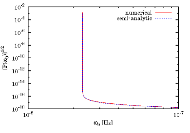
Figure 4: Gravitational power spectrum in the massive gravity with $M_{GW,0}=10^{10}H_{0}\sim 2\times 10^{-7}\,\text{Hz}$ shown with respect to $\omega_{0}$. The solid (red) curve is the spectrum obtained by the numerical calculation, and the dashed (blue) curve is the semi-analytical spectrum given by Eq. (46), where the GR spectrum is calculated numerically and the enhancement factor ${\cal S}(\omega_{0})$ is given analytically by Eqs. (50), (55) and (60).

Since the plot in Fig. 4 is shown with respect to $\omega_{0}\sim[(k/a_{0})^{2}+M_{GW,0}^{2}]^{1/2}$, most of the peak structure in the spectrum is compressed to a narrow region at $\omega_{0}\sim M_{GW,0}$ and its detailed structure is too subtle to see. To make the fine structure of the peak manifest, we show the plots with respect to $k$ in Fig. 5. We can see that the $k$ dependence changes at $k_{0}$ and $k_{c}$ as prescribed in Sec. IV, and that the semi-analytical result well reproduces the numerical one.

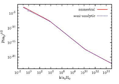
Figure 5: The gravitational power spectra in the massive gravity theory with $M_{GW,0}=10^{10}H_{0}\sim 2\times 10^{-7}\,\text{Hz}$ shown with respect to $k/a_{0}H_{0}$. The spectra are obtained by the numerical calculation (solid red) and semi-analytic estimate by Eqs. (46), (50), (55) and (60) (dotted blue), respectively. For the latter, the GR spectrum is calculated numerically and the enhancement factor ${\cal S}(\omega_{0})$ is calculated analytically.

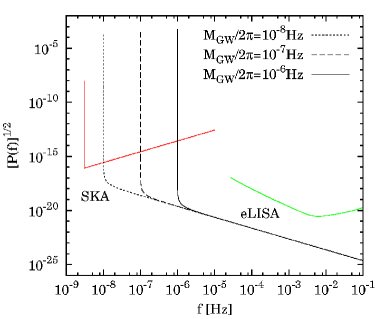
Figure 6: Gravitational power spectra for $M_{GW,0}/2\pi=10^{-8},10^{-7},10^{-6}\,\text{Hz}$ shown with sensitivity curves of future experiments. The curves are plotted assuming 10-years run of pulsar timing array with SKA Sesana:2010mx and 2-years run of eLISA AmaroSeoane:2012km . For the primordial spectra, we consider the tensor-to-scalar ratio to be $0.1$ and $e^{-N_{extra}}=10^{-1}$.

Before closing this section, we briefly comment on the observability of the peak feature in the spectrum. As seen from Fig. 6, the peak is observable by the pulsar timing if the mass is in the range of Eq. (65). For example, for the case of $M_{GW,0}=10^{-8}\,{\rm Hz}$ and a primordial spectrum with an IR cutoff at $k/a_{0}=1/H_{0}$, we find that the enhancement factor ${\cal S}(\omega_{0})$ reaches $\sim 10^{13}$. Since the enhancement is so large, we can expect the peak to be observable even when the tensor-to-scalar ratio takes much smaller value. The signal might be observable also for eLISA if its sensitivity could be extended to lower frequencies.

Note that, due to the finiteness of the observation time $T_{obs}$, the observed peak in the Fourier space is smoothed with a width of $\Delta f\sim 1/T_{obs}$. The signal would be detectable even after taking this effect into account if the amplification is sufficiently large. For example, following the calculations in Ref. Jenet:2005pv which discussed the pulsar timing observations, we find that the total RMS fluctuation of the timing residuals induced by the stochastic gravitational wave background is amplified relative to GR by a factor $\sim 10^{-4}\times(T_{obs}/H_{0})^{-4}(M_{GW,0}/H_{0})^{-3}\log(e^{N_{extra}}M_{GW,0}/H_{0})$. For $M_{GW,0}\gtrsim 10^{-8}\,\mathrm{Hz}$, this factor becomes large enough for the signal to be detectable by the cross correlation analysis using PPTA argued in Ref. Jenet:2005pv unless the tensor-to-scalar ratio is extremely small.

VI Summary and discussions

In this paper, we discussed how to probe the graviton mass using the gravitational wave observations. Our results are based on a general quadratic action given by Eq. (5) in which the graviton mass can be time-dependent, and thus they apply universally to any massive gravity theories in which modification from GR appears primarily in the tensor modes. The salient feature of the result is the sharp peak in the gravitational wave spectrum, whose position and height may tell us about the graviton mass of today and the length of the inflationary period. In Sec. V, we confirmed our analytical results match well with the numerical results which do not assume the thin-horizon approximation, and also argued the observability of the gravitational wave signal for various observatories. It would be interesting to apply the results to explicit examples of nonlinear completion of massive gravity theories and to derive constraints on such models based on the gravitational wave observations.

Although the example discussed in Sec. III (as well as in Ref. Gumrukcuoglu:2011zh ) was recently shown to suffer from nonlinear instabilities DGM , it is expected that other working examples exist. A construction with no extra polarization with respect to GR was discussed in Dubovsky:2004sg , where a constant mass contribution appears in the dispersion relations of the gravitational waves. Another potential example is the scenario considered in deRham:2012kf , where the scalar mode is rendered redundant by introduction of some symmetry. Although the vector graviton degrees are still present in this construction, the lack of the scalar graviton would relax the bounds from solar system tests.

Below, we briefly discuss other probes which are sensitive to $M_{GW}(t)$ at the time other than today. One interesting probe is the cosmic microwave background (CMB), especially its B-mode polarization spectrum which is sourced solely by gravitational waves. The signatures in CMB spectrum in the case of the constant mass $M_{GW}$ was discussed by Ref. Dubovsky:2009xk . Following the argument to derive the B-mode spectrum and generalizing it to the case of time-dependent mass term, we find that the main contribution to the spectrum is sensitive to the value of the mass at the time of the recombination. The most interesting observational feature will be obtained when the graviton mass at that time is in the range $(10\text{Mpc})^{-1}<M_{GW}<(10\text{Kpc})^{-1}$. For such a value of $M_{GW}$, the contribution to the B-mode spectrum from the gravitational wave increases compared to the GR case for the modes of low angular multipole $\ell$, and a plateau in the spectrum up to $\ell\lesssim 10^{-3}\times M_{GW}/H_{0}\sim 100$ is expected to emerge. There will be no signal for smaller values of $M_{GW}$, while for larger values, the entire spectrum will be suppressed, since the rapid oscillation of the gravitational wave, driven by the large $M_{GW}$, will average out the contribution to the CMB polarization spectrum.

Another interesting probe of the modification in tensor sector of gravity is the inspiralling compact binaries; the changes in the propagation speed due to the mass term will give rise to a modification in the evolution of the phase of the gravitational waves emitted by those binaries. Such an effect and the constraint on the constant graviton mass are argued in Ref. Will:1997bb . It may be interesting to generalize this analysis to the case of time-dependent graviton mass and discuss its observability for the future-planned gravitational wave observatories.

Finally, we give a brief comment on the time evolution of the gravitational wave energy density and a possible constraint on it. The energy spectrum of the gravitational wave defined with respect to wavenumber $k$ is given by

$$\Omega_{GW}(k,t)=\frac{1}{\rho_{\text{crit}}}\frac{d\rho_{GW}}{d\log k}=\frac{k^{3}}{12\pi H^{2}}\left(N^{-2}\dot{\gamma}_{k}^{2}+\omega^{2}\gamma_{k}^{2}\right)\propto k^{3}\omega^{2}\gamma_{k}^{2},$$ (66)

where $\omega$ is given by Eq. (24) and the final expression is valid for the WKB solution of Eq. (36). The ratio of the energy spectrum of the massive gravity relative to GR can be obtained following the derivations similar to Sec. IV. To discuss the constraint on the gravitational wave energy density coming from the Big Bang nucleosynthesis (BBN), we need to do the analysis taking $t$ to be the time of BBN. We assume that the gravitational wave primordial amplitude is given by Eq. (35), and consider the case that $M_{GW}(t)$ becomes larger than the Hubble scale before BBN. In such a case, the ratio is given by

$$\frac{\Omega_{GW}(k)}{\Omega_{GW}^{GR}(k)}=\begin{cases}1&(k_{0}<k)\\ k_{0}/k&(k_{c}<k<k_{0})\\ k_{0}/k_{c}&(k<k_{c})\end{cases}~{},$$ (67)

where $k_{0}$ and $k_{c}$ are defined in a similar manner with Sec. IV replacing $t_{0}$ by $t_{\text{BBN}}$. Roughly speaking, the total energy density of the gravitational wave becomes larger than that in GR by a factor of $k_{0}/k_{c}=M_{GW}(t_{\text{BBN}})/\sqrt{H_{\text{BBN}}M_{GW}(t_{c})}$ if $k_{c}$ is sufficiently large. Since the total energy density must satisfy $\int d(\log k)\Omega_{GW}(k)<10^{-5}$ at least Maggiore:1999vm , this enhancement of the gravitational wave energy density may give a tighter constraint on the primordial amplitude of the gravitational wave or the inflationary models from which it is derived. Obviously this constraint will be sensitive to $M_{GW}(t_{\text{BBN}})$. It may be interesting to pursue this issue using explicit examples of the massive gravity theories.

Appendix A Example from nonlinear massive gravity

In the nonlinear theory of massive gravity, the mass term not only introduces the effective mass to gravitational waves but also drives self-accelerating universes. In order to attribute the late-time acceleration of our universe to the self-acceleration from massive gravity, the effective cosmological constant $\Lambda_{\pm}$ due to the mass term should be set to the observed value:

$$\Lambda_{\pm}\sim H_{0}^{2}.$$ (68)

Therefore, a relevant question now is whether the nonlinear theory of massive gravity can simultaneously accommodate the effective mass in the preferred range (65) and the preferred value of the effective cosmological constant (68). These two quantities are given by the formulas (22) and (21), respectively. (For the sign of the effective cosmological constant in each branch, see Figure 1 of Ref. Gumrukcuoglu:2011zh .) Thus, for generic values of the parameters $\alpha_{3}$ and $\alpha_{4}$, the graviton mass $m_{g}$ in the action should be

$$m_{g}\sim H_{0},$$ (69)

and the quantity $r=H/(X_{\pm}H_{f})$ at present must be in the range

$$10^{20}<r_{0}<10^{28}.$$ (70)

where $r_{0}\equiv r(t_{0})$.

If we suppose that the primordial spectrum ${\cal P}_{prim}(k)$ of gravitational waves is generated by inflation then in order for the inflationary mechanism of generation of quantum fluctuations to work, the effective mass of gravitational waves must be sufficiently lower than the Hubble expansion rate during inflation. This is translated to the condition

$$r\ll\frac{H_{I}^{2}}{H_{0}^{2}}\quad\mbox{during inflation},$$ (71)

where $H_{I}$ is the Hubble expansion rate during inflation.

For example, if we demand the Poincaré symmetry in the field space as a global symmetry of the theory then the fiducial metric is restricted to Minkowski and the FRW background of the physical metric is inevitably an open universe Gumrukcuoglu:2011ew . In this case we have

$$r=\frac{Ha}{\sqrt{|K|}},$$ (72)

where $K$ ($<0$) is the spatial curvature constant. It is evident that $r$ increases during inflation and decreases after that (see footnote 3). Hence, the condition (70) implies that $r\gg 1$ throughout the evolution after inflation. In this case $M_{GW}^{2}\sim r\,m_{g}^{2}$ for the ’+’ branch (or $M_{GW}^{2}\sim-r\,m_{g}^{2}$ for the ’-’ branch), and the assumption (25) is actually satisfied, provided that $P\leq\rho$ and $m_{g}^{2}>0$ (or $m_{g}^{2}<0$, respectively).

Since $r$ decreases after inflation, the condition (71) leads to an upper bound on $r_{0}$. We thus need to see if such an upper bound on $r_{0}$ is consistent with the preferred range (70). For this purpose, supposing that the universe is dominated by inflaton oscillation (with the effective equation of state parameter $w=0$) between the end of inflation ($a=a_{f}$) and the onset of the radiation dominated epoch ($a=a_{R}$), the scale factor today is estimated by the entropy conservation as

$$\frac{a_{0}}{a_{f}}\sim g^{1/12}\frac{\sqrt{M_{Pl}H_{I}}}{T_{0}}\left(\frac{a_{R}}{a_{f}}\right)^{1/4},$$ (73)

where $T_{0}$ is the photon temperature today and $g$ is the number of relativistic degrees of freedom that eventually inject entropy to photons. By using this formula, the bound (71) at the end of inflation $t=t_{f}$ is rewritten as

$$r_{0}=r_{f}\frac{H_{0}}{H_{I}}\frac{a_{0}}{a_{f}}\ll\frac{H_{I}}{H_{0}}\frac{a_{0}}{a_{f}}\sim g^{1/12}\frac{\sqrt{M_{Pl}H_{I}}}{T_{0}}\frac{H_{I}}{H_{0}}\left(\frac{a_{R}}{a_{f}}\right)^{1/4},$$ (74)

where $r_{f}=r(t_{f})$. For example, for $g^{1/12}=O(1)$ with the instantaneous reheating approximation $a_{R}\simeq a_{f}$, this leads to

$$r_{0}\ll 10^{84}\times\left(\frac{H_{I}}{10^{13}GeV}\right)^{3/2},$$ (75)

and is consistent with the preferred range (70). Thus, in this simple example with Minkowski fiducial metric, the range (70) is consistent with the inflationary generation mechanism of primordial gravitational waves.

Note that, by the formula (72), the extreme hugeness of $r_{0}$ implied by the preferred range (70) is translated to the extreme flatness of our universe today: $10^{-56}<|\Omega_{tot}-1|<10^{-40}$. Thus, the number of e-folds during inflation must be much more than what is needed to solve the flatness problem. The preferred range (70) corresponds to the number of extra e-folds $\sim\ln r_{0}$ in the range

$$45<N_{extra}<65.$$ (76)

With this large number of extra e-folds, the primordial spectrum ${\cal P}_{prim}(k)$ of gravitational waves is expected to continue to a far infrared. Therefore, from the discussion in subsection IV.6 we conclude that the peak just above $\omega_{0}=M_{GW,0}$ should be rather high. Concretely, ${\cal P}_{prim}(k)$ is expected to continue down to $k\sim a_{0}H_{0}e^{-N_{extra}}$. By the formula (60), this corresponds to the large enhancement at the peak,

$${\cal S}_{peak}\sim\frac{a_{c}}{a_{k_{0}}^{GR}}\frac{\sqrt{k_{0}k_{c}}}{a_{0}H_{0}}e^{N_{extra}}\sim\frac{a_{c}}{a_{k_{0}}^{GR}}\frac{\sqrt{k_{0}k_{c}}}{a_{0}H_{0}}r_{0}.$$ (77)

Appendix B General fiducial metric

B.1 FRW-type fiducial metric

The background equation of motion for a general fiducial metric is derived in the Appendix A.1 of Ref. Gumrukcuoglu:2011zh . We briefly summarize that derivation for reference.

We consider a FRW-type fiducial metric given by

$$f_{\mu\nu}=-\hat{n}^{2}(\hat{\phi}^{0})\partial_{\mu}\hat{\phi}^{0}\partial_{\nu}\hat{\phi}^{0}+\hat{\alpha}^{2}(\hat{\phi}^{0})\Omega_{ij}^{(K)}\partial_{\mu}\hat{\phi}^{i}\partial_{\nu}\hat{\phi}^{j},$$ (78)

where $\hat{n}$ and $\hat{\alpha}$ are general functions of $\hat{\phi}^{0}$. Applying the field redefinition given by $(\hat{\phi}^{0},\hat{\phi}^{i})=(f(\phi^{0}),\phi^{i})$, where $f$ is a function to be determined, and taking the gauge $\phi^{\mu}=x^{\mu}$, the fiducial metric of Eq. (78) becomes

$$f_{\mu\nu}dx^{\mu}dx^{\nu}=-\hat{n}^{2}\bigl{(}f(t)\bigr{)}\dot{f}(t)^{2}dt^{2}+\hat{\alpha}^{2}\bigl{(}f(t)\bigr{)}\Omega^{(K)}_{ij}dx^{i}dx^{j},$$ (79)

where the dot ($\,\dot{}\,$) denotes the derivative with respect to $t$. For this fiducial metric, the matrix $\mathcal{K}^{\mu}_{~{}\nu}$ becomes

$$\mathcal{K}^{\mu}_{~{}\nu}=\text{Diag}\left(\zeta,\xi,\xi,\xi\right),\qquad\zeta=1-\frac{\hat{n}\dot{f}}{N},\qquad\xi=1-\frac{\hat{\alpha}}{a}.$$ (80)

Then, up to boundary terms the gravity action reduces to

$$I_{g}=\int d^{3}x\sqrt{\Omega}\left(3KNa-\frac{3a\dot{a}^{2}}{N}+m_{g}^{2}L_{g}\right),$$ (81)

where

$$L_{g}=Na^{3}\left(\mathcal{L}_{2}+\alpha_{3}\mathcal{L}_{3}+\alpha_{4}\mathcal{L}_{4}\right),\qquad\mathcal{L}_{2}=3\xi(\zeta+\xi),\qquad\mathcal{L}_{3}=\xi^{2}(3\zeta+\xi),\qquad\mathcal{L}_{4}=\zeta\xi^{3}.$$ (82)

The variation of this action with respect to $f$ yields

$$0 =\frac{\partial L_{g}}{\partial\zeta}\frac{\partial\zeta}{\partial f}+\frac{\partial L_{g}}{\partial\xi}\frac{\partial\xi}{\partial f}-\left(\frac{\partial L_{g}}{\partial\zeta}\frac{\partial\zeta}{\partial\dot{f}}\right)^{\text{\large$\cdot$}}=3Na^{2}\left(aH-\alpha\hat{H}_{f}\right)\left[1+2\xi+\alpha_{3}(2+\xi)\xi+\alpha_{4}\xi^{2}\right],$$ (83)

where $H$ and $H_{f}$ are the Hubble parameters of the physical and fiducial metrics defined by

$$H(t)\equiv\frac{\dot{a}}{Na},\qquad\hat{H}_{f}\bigl{(}f(t)\bigr{)}\equiv\frac{\hat{\alpha}^{\prime}}{\hat{n}\hat{\alpha}}\quad~{}~{}\left(\hat{\alpha}^{\prime}\equiv\frac{d\hat{\alpha}}{d\hat{\phi}^{0}}\right).$$ (84)

Below, we focus on the solution of Eq. (83) given by

$$1+2\xi+\alpha_{3}\xi(2+\xi)+\alpha_{4}\xi^{2}=0,$$ (85)

whose solution is given by

$$X_{\pm}=1-\xi=\frac{\hat{\alpha}\bigl{(}f(t)\bigr{)}}{a(t)},\qquad X_{\pm}\equiv\frac{1+2\alpha_{3}+\alpha_{4}\pm\sqrt{1+\alpha_{3}+\alpha_{3}^{2}-\alpha_{4}}}{\alpha_{3}+\alpha_{4}}.$$ (86)

Varying the action with respect to $N$ and $a$ and using the solution of Eq. (86), we obtain Eq. (20) as the background equations. The second equation in Eq. (20) is consistent with the first one if the matter fluid obeys usual conservation law $\dot{\rho}+3(\dot{a}/a)(\rho+p)=0$. The evolution of $a$ is determined by Eq. (20) for given $N$, and it determines $f(t)$ via Eq. (86). Note that $\hat{n}(f(t))$, $\hat{\alpha}(f(t))$ and $\hat{H}_{f}(f(t))$ correspond to $n(t)$, $\alpha(t)$ and $H_{f}(t)$ of Sec. II, respectively. (Almost equivalently, we may set $f(t)=t$ and regard $\hat{\alpha}(t)$ and $\hat{n}(t)$ are given functions. In this case, Eq. (86) and the Friedmann equation in Eq. (20) are regarded as equations to fix $a(t)$ and $N(t)$, respectively.)

One example of the fiducial metric of this type is the Minkowski metric in the open chart ($K<0$) given by Gumrukcuoglu:2011ew

$$f_{\mu\nu}=-\partial_{\mu}\varphi^{0}\partial_{\nu}\varphi^{0}+\delta_{ij}\partial_{\mu}\varphi^{i}\partial_{\nu}\varphi^{j}=-{f^{\prime}}^{2}(\phi^{0})\partial_{\mu}\phi^{0}\partial_{\nu}\phi^{0}+|K|f^{2}(\phi^{0})\Omega_{ij}^{(K)}dx^{i}dx^{j},$$ (87)

where we used the field redefinition given by

$$\varphi^{0}=f(\phi^{0})\sqrt{1-K\delta_{ij}\phi^{i}\phi^{j}},\qquad\varphi^{i}=\sqrt{-K}f(\phi^{0})\phi^{i}.$$ (88)

Taking the gauge $\phi^{i}=x^{i}$, we find Eq. (86) becomes $X_{\pm}=\sqrt{|K|}f(t)/a(t)$, which determines $f(t)$ in terms of $a(t)$. The Friedmann equation, Eq. (20), holds as it is. In this case we have $n(\phi^{0})=|f^{\prime}(\phi^{0})|$ and $\alpha(\phi^{0})=\sqrt{|K|}f(\phi^{0})$, and thus $H_{f}=\text{sign}(f^{\prime})/f=\text{sign}(f^{\prime})\sqrt{|K|}/X_{\pm}a$.

B.2 (Anti-)de Sitter fiducial metric

In this section, we comment that the fiducial metric of Eq. (17) for any $K$ can be obtained from a single de Sitter metric, and the for $K>0$ can be obtained from the anti-de Sitter metric.

We begin with the de Sitter fiducial metric with flat spatial section given by

$$f_{\mu\nu}=-\partial_{\mu}\varphi^{0}\partial_{\nu}\varphi^{0}+\exp\bigl{(}2\bar{H}_{f}{\varphi^{0}}\bigr{)}\delta_{ij}\partial_{\mu}\varphi^{i}\partial_{\nu}\varphi^{j}.$$ (89)

By the redefinition $\varphi^{0}=f(\phi^{0})$ and $\varphi^{i}=\phi^{i}$, this fiducial metric takes the form of Eq. (17) with $K=0$, $H_{f}=\bar{H}_{f}$, $n=\bigl{|}\dot{f}\bigr{|}$ and $\alpha=\exp\bigl{(}2\bar{H}_{f}f(\phi^{0})\bigr{)}$.

Assuming $K>0$, the field redefinition given by

$$\varphi^{0}=\bar{H}_{f}^{-1}\log\left[\sinh f(\phi^{0})+\cosh f(\phi^{0})\sqrt{1-K\delta_{ij}\phi^{i}\phi^{j}}\right],\qquad\varphi^{i}=\frac{\bar{H}_{f}^{-1}\sqrt{K}\phi_{i}}{\tanh f(\phi^{0})+\sqrt{1-K\delta_{ij}\phi^{i}\phi^{j}}}$$ (90)

makes the fiducial metric of Eq. (89) into

$$f_{\mu\nu}=\bar{H}_{f}^{-2}\left(-{f^{\prime}}^{2}(\phi^{0})\partial_{\mu}\phi^{0}\partial_{\nu}\phi^{0}+K\cosh^{2}\!f(\phi^{0})\,\Omega^{(K)}_{ij}\partial_{\mu}\phi^{i}\partial_{\nu}\phi^{j}\right),$$ (91)

which is of the form of Eq. (17) with $K>0$ and $H_{f}=\bar{H}_{f}\tanh f(\phi^{0})$. The counterpart of Eq. (86) for Eq. (91) is given by

$$X_{\pm}=\frac{\sqrt{K}}{\bar{H}_{f}}\frac{\cosh\bigl{(}f(t)\bigr{)}}{a(t)},$$ (92)

and the Friedmann equation, Eq. (20), holds as it is.

Similarly, for $K<0$, the redefinition given by

$$\varphi^{0}=\bar{H}_{f}\log\left[\cosh f(\phi^{0})+\sinh f(\phi^{0})\sqrt{1-K\delta_{ij}\phi^{i}\phi^{j}}\right],\qquad\varphi^{i}=\frac{\bar{H}_{f}^{-1}\sqrt{|K|}\phi^{i}}{\coth f(\phi^{0})+\sqrt{1-K\delta_{ij}\phi^{i}\phi^{j}}}$$ (93)

makes Eq. (89) into

$$f_{\mu\nu}=\bar{H}_{f}^{-2}\left[-{f^{\prime}}^{2}(\phi^{0})\partial_{\mu}\phi^{0}\partial_{\nu}\phi^{0}+|K|\sinh^{2}\!f(\phi^{0})\,\Omega^{(K)}_{ij}\partial_{\mu}\phi^{i}\partial_{\nu}\phi^{j}\right],$$ (94)

which is of the form of Eq. (17) with $K<0$ and $H_{f}=\bar{H}_{f}\coth f(\phi^{0})$. The counterpart of Eq. (86) is given by

$$X_{\pm}=\frac{\sqrt{|K|}}{\bar{H}_{f}}\frac{\sinh\bigl{(}f(t)\bigr{)}}{a(t)}.$$ (95)

Next, we consider the anti-de Sitter (AdS) fiducial metric given by

$$f_{\mu\nu}=-\left(1+k^{2}\delta_{ij}\varphi^{i}\varphi^{j}\right)\partial_{\mu}\varphi^{0}\partial_{\nu}\varphi^{0}+\Omega^{(-k^{2})}_{ij}\partial_{\mu}\varphi^{i}\partial_{\nu}\varphi^{j},$$ (96)

which is the AdS metric with curvature $k$ in the global chart. Assuming $K<0$, the field redefinition given by

$$\varphi^{0}=k\arcsin\left(\frac{\sin f(\phi^{0})}{\sqrt{1-K\cos^{2}\!f(\phi^{0})\,\delta_{ij}\phi^{i}\phi^{j}}}\right),\qquad\varphi^{i}=\frac{\sqrt{|K|}}{k}\cos\!f(\phi^{0})\,\phi^{i}$$ (97)

make the fiducial metric into

$$f_{\mu\nu}=k^{-2}\left(-{f^{\prime}}^{2}(\phi^{0})\partial_{\mu}\phi^{0}\partial_{\nu}\phi^{0}+\left|K\right|\cos^{2}\!f(\phi^{0})\,\Omega^{(K)}_{ij}\partial_{\mu}\phi^{i}\partial_{\nu}\phi^{j}\right),$$ (98)

for which $H_{f}=k\tan f(\phi^{0})$ and the counterpart of Eq. (86) is

$$X_{\pm}=\frac{\sqrt{\left|K\right|}}{k}\frac{\cos f(t)}{a(t)}.$$ (99)

We summarize these results in Table 1. Note the the constraint equations, which are the counterparts of Eq. (86), give restrictions on the trajectory of $a(t)$. For example, the constraint equation in the $K>0$ case allows only the trajectory of $a(t)$ which starts from the infinity, decreases to the minimum and grows to the infinity again. Even though the $a(t)$ which starts from zero, increases to the maximum and comes back to zero is also allowed by the Friedmann equation, it is not consistent with the constraint equation and is not a cosmological solution in this model.

Table 1: Results summary.

		$\varphi^{0}$	$\varphi^{i}$	$H_{f}$	Constraint eq.
	$K>0$	$\bar{H}_{f}^{-1}\log\left[\sinh f(\phi^{0})+\cosh f(\phi^{0})\sqrt{1-K\delta_{ij}\phi^{i}\phi^{j}}\right]$	$\frac{\bar{H}_{f}^{-1}\sqrt{K}\phi^{i}}{\tanh f(\phi^{0})+\sqrt{1-K\delta_{ij}\phi^{i}\phi^{j}}}$	$\bar{H}_{f}\tanh\bigl{(}f(\phi^{0})\bigr{)}$	$X_{\pm}=\frac{\sqrt{K}}{\bar{H}_{f}}\frac{\cosh f(t)}{a(t)}$
dS	$K=0$	$f(\phi^{0})$	$\phi^{i}$	$\bar{H}_{f}$	$X_{\pm}=\frac{\exp(\bar{H}_{f}f(t))}{a(t)}$
	$K<0$	$\bar{H}_{f}^{-1}\log\left[\cosh f(\phi^{0})+\sinh f(\phi^{0})\sqrt{1-K\delta_{ij}\phi^{i}\phi^{j}}\right]$	$\frac{\bar{H}_{f}^{-1}\sqrt{|K|}\phi^{i}}{\coth f(\phi^{0})+\sqrt{1-K\delta_{ij}\phi^{i}\phi^{j}}}$	$\bar{H}_{f}\coth\bigl{(}f(\phi^{0})\bigr{)}$	$X_{\pm}=\frac{\sqrt{\left|K\right|}}{\bar{H}_{f}}\frac{\sinh f(t)}{a(t)}$
AdS	$K<0$	$k\arcsin\left(\frac{\sin f(\phi^{0})}{\sqrt{1-K\cos^{2}f(\phi^{0})\delta_{ij}\phi^{i}\phi^{j}}}\right)$	$\frac{\sqrt{|K|}}{k}\cos f(\phi^{0})\phi^{i}$	$k\tan f(\phi^{0})$	$X_{\pm}=\frac{\sqrt{\left|K\right|}}{k}\frac{\cos f(t)}{a(t)}$

Before closing this appendix, we briefly mention some examples of $M_{GW}$. For instance, in the case of the $+$ blanch solution with the Minkowski fiducial metric,

$$\left.M^{2}_{GW}\right|_{\rm Minkowski}\propto\left(\dot{a}+{\rm constant}\right)\,.$$ (100)

As a result, $a^{2}|M^{2}_{GW}|$ always grows with time, provided that the dominant fluid’s equation of state is $w<1$. Another example is the de Sitter fiducial metric, for which we have

$$\left.M^{2}_{GW}\right|_{\rm deSitter}\propto\left(\frac{\dot{a}}{a}+{\rm constant}\right)\,.$$ (101)

In this case, the contribution from the first term in $a^{2}M^{2}_{GW}$ will grow if $w<1/3$. Although for radiation dominated universe, this contribution is constant, the second term will still grow as $a^{2}$. In the light of these examples and the late-time stability of the system, we adopt the assumption (25) throughout this paper.

Appendix C Analytic solutions of $\gamma_{k}$

We show the analytic solution for Eq. (9) for power-law type $M_{GW}^{2}=M_{\text{eq}}^{2}(a/a_{\text{eq}})^{p}$, which covers the simple examples such as the constant $M_{GW}$ and also the examples mentioned above. The aim of this section is to confirm the validity of the thin-horizon approximation used in Sec. IV.

We define the conformal time $\eta$ from the scale factor $a=a_{\text{eq}}(t/t_{\text{eq}})^{1/2}$ (RD) and $a=a_{\text{eq}}(t/t_{\text{eq}})^{3/2}$ (MD) as

$$\eta\equiv\alpha\int_{0}^{t}\frac{dt}{a(t)}=\eta_{\text{eq}}\times\begin{cases}\frac{a}{a_{\text{eq}}}&(\text{RD})\\ \frac{2}{3}\left(\frac{a}{a_{\text{eq}}}\right)^{1/2}-\frac{1}{2}&(\text{MD})\end{cases}\qquad\Leftrightarrow\qquad\frac{a}{a_{\text{eq}}}=\begin{cases}\frac{\eta}{\eta_{\text{eq}}}&(\text{RD})\\ \left(\frac{2}{3}\left(\frac{\eta}{\eta_{\text{eq}}}+\frac{1}{2}\right)\right)^{2}&(\text{MD})\end{cases}~{},$$ (102)

where $\alpha$ is a constant and $\eta_{\text{eq}}\equiv 2\alpha t_{\text{eq}}/a_{\text{eq}}$.

We consider the case that $M_{GW}$ becomes dominant in the MD era first. Eq. (9) in this case becomes

$$\bar{\gamma}_{k}^{\prime\prime}+\left(k^{2}+a^{2}M_{\text{eq}}^{2}\left(\frac{a}{a_{\text{eq}}}\right)^{p}-\frac{a^{\prime\prime}}{a}\right)\bar{\gamma}_{k}=0\qquad\Leftrightarrow\qquad\frac{d^{2}\bar{\gamma}_{k}}{d\hat{\eta}^{2}}+\left(\hat{k}^{2}+\left(\frac{2}{3}\right)^{2(p+2)}\hat{M}_{\text{eq}}^{2}\hat{\eta}^{2(p+2)}-\frac{2}{\hat{\eta}^{2}}\right)\bar{\gamma}_{k}=0,$$ (103)

where we introduced $\hat{k}\equiv k\eta_{\text{eq}}$, $\hat{M}_{\text{eq}}\equiv a_{\text{eq}}\eta_{\text{eq}}M_{\text{eq}}$, $\hat{a}\equiv a/a_{\text{eq}}$ and $\hat{\eta}\equiv\frac{\eta}{\eta_{\text{eq}}}+\frac{1}{2}=2\hat{a}^{1/2}/3$. Below, we use an approximation depending on which of $k$ and $aM_{GW}$ is dominant at the moment of the horizon crossing.

1. $k\gg aM_{GW}$ at the horizon crossing:

   In this case, Eq. (103) is approximated near the moment of the horizon crossing as

   $$\frac{d^{2}\bar{\gamma}_{k}}{d\hat{\eta}^{2}}+\left(\hat{k}^{2}-\frac{2}{\hat{\eta}^{2}}\right)\bar{\gamma}_{k}=0,$$ (104)

   which is same as that in the pure GR. This equation has an exact solution which becomes regular for $\hat{k}\hat{\eta}\to 0$ given by

   $$\bar{\gamma}_{k}=C\times\frac{3}{\hat{k}^{2}}\left(-\cos\bigl{(}\hat{k}\hat{\eta}\bigr{)}+\frac{\sin\bigl{(}\hat{k}\hat{\eta}\bigr{)}}{\hat{k}\hat{\eta}}\right)\bar{\gamma}_{k}\xrightarrow{\hat{k}\hat{\eta}\ll 1}C\hat{\eta}^{2}.$$ (105)

   The primordial amplitude is given by $|\gamma_{k}|=k^{-3/2}(H_{*}/M_{Pl})$ and

   $$\left|\bar{\gamma}_{k}\right|=\frac{H_{*}a}{k^{3/2}M_{Pl}}=\frac{4H_{*}a_{\text{eq}}\eta_{\text{eq}}^{3/2}}{9M_{Pl}\hat{k}^{3/2}}\hat{\eta}^{2}\equiv\bar{\gamma}_{*}\hat{\eta}^{2},$$ (106)

   and then we may identify it with the right-hand side of Eq. (105) in the limit of $\hat{k}\hat{\eta}\ll 1$. The solution in the WKB regime, on the other hand, is given by

   $$\bar{\gamma}_{k}=\frac{C^{\prime}}{\sqrt{\hat{\tilde{k}}}}\cos\left(\int\hat{\tilde{k}}d\hat{\eta}\right),$$ (107)

   where $\hat{\tilde{k}}^{2}\equiv(k^{2}+a^{2}M_{GW}^{2})\eta_{\text{eq}}^{2}$. Comparing it with Eq. (105) in the limit of $\hat{k}\hat{\eta}\gg 1$, we may fix the coefficient $C^{\prime}$ to have

   $$\bar{\gamma}_{k}=\frac{3\bar{\gamma}_{*}}{\hat{k}^{3/2}}\cos\left(\int\hat{\tilde{k}}d\hat{\eta}\right).$$ (108)

   Let us compare Eq. (108) with $\gamma_{k}$ obtained using the thin-horizon approximation. The condition to determine $a$ at the horizon crossing is given by $k=a\hat{H}=a^{\prime}/a=2/\eta$. Matching the WKB solution with the primordial solution at $\eta$ defined by this equation, we find the solution is given by

   $$\bar{\gamma}_{k}=\frac{4\bar{\gamma}_{*}}{\hat{k}^{3/2}}\cos\left(\int\hat{\tilde{k}}d\hat{\eta}\right),$$ (109)

   which coincide with Eq. (108) up to a numerical factor.

2. $aM_{GW}\gg k$ at the horizon crossing:

   Eq. (103) in this case is approximated as

   $$\bar{\gamma}^{\prime\prime}_{k}+\left(a^{2}M_{GW}^{2}-\frac{a^{\prime\prime}}{a}\right)\bar{\gamma}=0\qquad\Leftrightarrow\qquad\frac{d\bar{\gamma}}{d\hat{\eta}^{2}}+\left(\left(\frac{2}{3}\right)^{2(p+2)}\hat{M}_{\text{eq}}^{2}\hat{\eta}^{2(p+2)}-\frac{2}{\hat{\eta}^{2}}\right)\bar{\gamma}_{k}=0,$$ (110)

   which have an exact solution that becomes regular for $\hat{k}\hat{\eta}\to 0$ given by

   $$\bar{\gamma}_{k}=C\times\frac{\left(\frac{3}{2}\right)^{\frac{3}{2}-\frac{3}{q}}q^{\frac{3}{q}}\Gamma\left(1+\frac{3}{q}\right)}{\hat{M}_{\text{eq}}^{\frac{3}{q}}}~{}\hat{\eta}^{1/2}J_{\frac{3}{q}}\left(\frac{3\left(\frac{2}{3}\right)^{\frac{q}{2}}\hat{M}_{\text{eq}}}{q}\hat{\eta}^{\frac{q}{2}}\right)\xrightarrow{\hat{\eta}\to 0}C\hat{\eta}^{2},$$ (111)

   where $J$ is the Bessel function and we have defined $q\equiv 2(p+3)$. Fixing $C$ using Eq. (106), we find $\bar{\gamma}_{k}$ to be

   $$\bar{\gamma}_{k}=\bar{\gamma}_{*}\times\frac{\left(\frac{3}{2}\right)^{\frac{3}{2}-\frac{3}{q}}q^{\frac{3}{q}}\Gamma\left(1+\frac{3}{q}\right)}{\hat{M}_{\text{eq}}^{\frac{3}{q}}}~{}\hat{\eta}^{1/2}J_{\frac{3}{q}}\left(\frac{3\left(\frac{2}{3}\right)^{\frac{q}{2}}\hat{M}_{\text{eq}}}{q}\hat{\eta}^{\frac{q}{2}}\right)\\ \xrightarrow{\hat{\eta}\to\infty}\frac{q^{\frac{3}{q}+\frac{1}{2}}\Gamma\left(1+\frac{3}{q}\right)}{\sqrt{\pi}}\times\frac{\bar{\gamma}_{*}\left(\frac{3}{2}\right)^{\frac{3}{2}-\frac{3}{q}}\hat{M}_{\text{eq}}^{-\frac{3}{q}}}{\sqrt{\left(\frac{2}{3}\right)^{\frac{q}{2}-1}\hat{M}_{\text{eq}}\hat{\eta}^{\frac{q}{2}-1}}}\cos\left(\frac{3\left(\frac{2}{3}\right)^{\frac{q}{2}}\hat{M}_{\text{eq}}}{q}\hat{\eta}^{\frac{q}{2}}\right),$$ (112)

   where we neglected the phase of the oscillation. This expression is valid as long as $M_{GW}$ dominates over $k/a$.

   Below, we compare it with the expression obtained from the thin-horizon approximation. The condition to determine $\eta$ at the horizon crossing is given by

   $$\left(\frac{2}{3}\right)^{2(p+2)}\hat{M}_{\text{eq}}^{2}\hat{\eta}^{2(p+2)}=\frac{2}{\hat{\eta}^{2}}\qquad\therefore\quad\eta=2^{\frac{1}{2(p+3)}}\left(\frac{3}{2}\right)^{\frac{p+2}{p+3}}\hat{M}_{\text{eq}}^{-\frac{1}{p+3}}.$$ (113)

   Matching the WKB solution with the primordial solution at this $\eta$, we find

   $$\bar{\gamma}_{k}=2^{\frac{1}{4}+\frac{3}{2q}}\times\frac{\bar{\gamma}_{*}\left(\frac{3}{2}\right)^{\frac{3}{2}-\frac{3}{q}}\hat{M}_{\text{eq}}^{-\frac{3}{q}}}{\sqrt{\hat{\tilde{k}}}}\cos\left(\int\hat{\tilde{k}}d\hat{\eta}\right).$$ (114)

   This expression coincides with Eq. (112) up to an $\mathcal{O}(1)$ factor for generic $q>0$, and thus the thin-horizon approximation is fairly good even in this case.

Finally, we briefly comment on the case that $M_{GW}$ becomes dominant in the RD era. In this case, Eq. (9) becomes $\bar{\gamma}^{\prime\prime}+\left(k^{2}+a^{2}M_{GW}^{2}\right)\bar{\gamma}=0$. As long as $k^{2}+a^{2}M_{GW}^{2}$ is positive and its time variation is sufficiently slow, the solution will be well approximated by the WKB solution. The amplitude of this solution is determined by matching it to the primordial solution. By construction, this solution will be well approximated by the solution given by the thin-horizon approximation in general.

References

- (1) M. Fierz and W. Pauli, Proc. Roy. Soc. Lond. A 173, 211 (1939).
- (2) D. G. Boulware, S. Deser, Phys. Rev. D6, 3368-3382 (1972).
- (3) C. de Rham, G. Gabadadze, Phys. Rev. D82, 044020 (2010). [arXiv:1007.0443 [hep-th]].
- (4) C. de Rham, G. Gabadadze, A. J. Tolley, Phys. Rev. Lett. 106, 231101 (2011). [arXiv:1011.1232 [hep-th]].
- (5) S. F. Hassan, R. A. Rosen, [arXiv:1106.3344 [hep-th]].
- (6) C. de Rham, G. Gabadadze, A. Tolley, [arXiv:1107.3820 [hep-th]].
- (7) C. de Rham, G. Gabadadze, A. J. Tolley, [arXiv:1108.4521 [hep-th]].
- (8) S. F. Hassan, R. A. Rosen, A. Schmidt-May, [arXiv:1109.3230 [hep-th]].
- (9) S. F. Hassan and R. A. Rosen, JHEP 1204, 123 (2012) [arXiv:1111.2070 [hep-th]].
- (10) M. Mirbabayi, arXiv:1112.1435 [hep-th].
- (11) A. Golovnev, Phys. Lett. B 707, 404 (2012) [arXiv:1112.2134 [gr-qc]].
- (12) J. Kluson, JHEP 1206, 170 (2012) [arXiv:1112.5267 [hep-th]]; J. Kluson, Phys. Rev. D 86, 044024 (2012) [arXiv:1204.2957 [hep-th]].
- (13) C. de Rham, G. Gabadadze, L. Heisenberg, D. Pirtskhalava, Phys. Rev. D83, 103516 (2011). [arXiv:1010.1780 [hep-th]].
- (14) K. Koyama, G. Niz, G. Tasinato, Phys. Rev. Lett. 107, 131101 (2011). [arXiv:1103.4708 [hep-th]].
- (15) T. .M. Nieuwenhuizen, Phys. Rev. D84, 024038 (2011). [arXiv:1103.5912 [gr-qc]].
- (16) K. Koyama, G. Niz, G. Tasinato, Phys. Rev. D84, 064033 (2011). [arXiv:1104.2143 [hep-th]].
- (17) A. H. Chamseddine, M. S. Volkov, Phys. Lett. B704, 652-654 (2011). [arXiv:1107.5504 [hep-th]].
- (18) G. D’Amico, C. de Rham, S. Dubovsky, G. Gabadadze, D. Pirtskhalava and A. J. Tolley, Phys. Rev. D 84, 124046 (2011) [arXiv:1108.5231 [hep-th]].
- (19) A. E. Gumrukcuoglu, C. Lin and S. Mukohyama, JCAP 1111, 030 (2011) [arXiv:1109.3845 [hep-th]].
- (20) K. Koyama, G. Niz and G. Tasinato, JHEP 1112, 065 (2011) [arXiv:1110.2618 [hep-th]].
- (21) D. Comelli, M. Crisostomi, F. Nesti and L. Pilo, Phys. Rev. D 85, 024044 (2012) [arXiv:1110.4967 [hep-th]].
- (22) M. S. Volkov, JHEP 1201, 035 (2012) [arXiv:1110.6153 [hep-th]].
- (23) M. von Strauss, A. Schmidt-May, J. Enander, E. Mortsell and S. F. Hassan, JCAP 1203, 042 (2012) [arXiv:1111.1655 [gr-qc]].
- (24) D. Comelli, M. Crisostomi, F. Nesti and L. Pilo, JHEP 1203, 067 (2012) [arXiv:1111.1983 [hep-th]].
- (25) L. Berezhiani, G. Chkareuli, C. de Rham, G. Gabadadze and A. J. Tolley, Phys. Rev. D 85, 044024 (2012) [arXiv:1111.3613 [hep-th]].
- (26) Y. Brihaye and Y. Verbin, arXiv:1112.1901 [gr-qc].
- (27) T. Kobayashi, M. Siino, M. Yamaguchi and D. Yoshida, arXiv:1205.4938 [hep-th].
- (28) N. Arkani-Hamed, H. -C. Cheng, M. A. Luty and S. Mukohyama, JHEP 0405, 074 (2004) [hep-th/0312099].
- (29) N. Arkani-Hamed, H. -C. Cheng, M. A. Luty, S. Mukohyama and T. Wiseman, JHEP 0701, 036 (2007) [hep-ph/0507120].
- (30) V. A. Rubakov, hep-th/0407104.
- (31) S. L. Dubovsky, JHEP 0410, 076 (2004) [hep-th/0409124].
- (32) A. De Felice, A. E. Gumrukcuoglu and S. Mukohyama, arXiv:1206.2080 [hep-th].
- (33) G. D’Amico, arXiv:1206.3617 [hep-th].
- (34) A. E. Gumrukcuoglu, C. Lin and S. Mukohyama, JCAP 1203, 006 (2012) [arXiv:1111.4107 [hep-th]].
- (35) D. Langlois and A. Naruko, arXiv:1206.6810 [hep-th].
- (36) D. Blas, D. Comelli, F. Nesti and L. Pilo, Phys. Rev. D 80, 044025 (2009) [arXiv:0905.1699 [hep-th]].
- (37) C. de Rham and S. Renaux-Petel, arXiv:1206.3482 [hep-th].
- (38) A. E. Gumrukcuoglu, C. Lin and S. Mukohyama, arXiv:1206.2723 [hep-th].
- (39) H. Motohashi and T. Suyama, arXiv:1208.3019 [hep-th].
- (40) S. L. Dubovsky, P. G. Tinyakov and I. I. Tkachev, Phys. Rev. D 72, 084011 (2005) [hep-th/0504067].
- (41) G. D. Moore and A. E. Nelson, JHEP 0109, 023 (2001) [hep-ph/0106220].
- (42) R. Kimura and K. Yamamoto, JCAP 1207, 050 (2012) [arXiv:1112.4284 [astro-ph.CO]].
- (43) G. W. Horndeski, Int. J. Theor. Phys. 10 (1974) 363-384.
- (44) T. Kobayashi, M. Yamaguchi and J. ’i. Yokoyama, Prog. Theor. Phys. 126, 511 (2011) [arXiv:1105.5723 [hep-th]].
- (45) P. Amaro-Seoane, S. Aoudia, S. Babak, P. Binetruy, E. Berti, A. Bohe, C. Caprini and M. Colpi et al., arXiv:1201.3621 [astro-ph.CO].
- (46) A. R. Taylor, A. R. 2008, IAU Symposium, 248, 164
- (47) G. B. Hobbs, M. Bailes, N. D. R. Bhat, S. Burke-Spolaor, D. J. Champion, W. Coles, A. Hotan and F. Jenet et al., arXiv:0812.2721 [astro-ph].
- (48) L. S. Finn and P. J. Sutton, Phys. Rev. D 65, 044022 (2002) [gr-qc/0109049].
- (49) T. Clifton, P. G. Ferreira, A. Padilla and C. Skordis, Phys. Rept. 513, 1 (2012) [arXiv:1106.2476 [astro-ph.CO]].
- (50) C. de Rham, A. J. Tolley and D. H. Wesley, arXiv:1208.0580 [gr-qc].
- (51) E. Komatsu et al. [WMAP Collaboration], Astrophys. J. Suppl. 192, 18 (2011) [arXiv:1001.4538 [astro-ph.CO]].
- (52) A. Sesana and A. Vecchio, Class. Quant. Grav. 27, 084016 (2010) [arXiv:1001.3161 [astro-ph.CO]].
- (53) F. A. Jenet, G. B. Hobbs, K. J. Lee and R. N. Manchester, Astrophys. J. 625, L123 (2005) [astro-ph/0504458].
- (54) S. Dubovsky, R. Flauger, A. Starobinsky and I. Tkachev, Phys. Rev. D 81, 023523 (2010) [arXiv:0907.1658 [astro-ph.CO]].
- (55) C. M. Will, Phys. Rev. D 57, 2061 (1998) [gr-qc/9709011].
- (56) S. L. Dubovsky, P. G. Tinyakov and I. I. Tkachev, Phys. Rev. Lett. 94, 181102 (2005) [hep-th/0411158].
- (57) M. Maggiore, Phys. Rept. 331, 283 (2000) [gr-qc/9909001].
- (58) M. Fasiello and A. J. Tolley, arXiv:1206.3852 [hep-th].