Onset of superconductivity in a voltage-biased NSN microbridge

Abstract

We study the stability of the normal state in a mesoscopic NSN junction biased by a constant voltage $V$ with respect to the formation of the superconducting order. Using the linearized time-dependent Ginzburg-Landau equation, we obtain the temperature dependence of the instability line, $V_{\text{inst}}(T)$, where nucleation of superconductivity takes place. For sufficiently low biases, a stationary symmetric superconducting state emerges below the instability line. For higher biases, the normal phase is destroyed by the formation of a non-stationary bimodal state with two superconducting nuclei localized near the opposite terminals. The low-temperature and large-voltage behavior of the instability line is highly sensitive to the details of the inelastic relaxation mechanism in the wire. Therefore, experimental studies of $V_{\text{inst}}(T)$ in NSN junctions may be used as an effective tool to access parameters of the inelastic relaxation in the normal state.

Nonequilibrium superconductivity has being attracting significant experimental and theoretical attention over decades Kopnin (2001); Gray (1981); Gulian and Zharkov (1999), ranging from vortex dynamics Langenberg and Larkin (1986) to the physics of the resistive state in current-carrying superconductors Vodolazov et al. (2003); Xiong et al. (1997); Rogachev et al. (2006); Li et al. (2011); Astafiev et al. (2012). It was recognized long ago Ivlev and Kopnin (1984) that a superconducting wire typically has a hysteretic current voltage characteristic specified by several “critical” currents. In an up-sweep, a current exceeding the thermodynamic depairing current, $I_{c}(T)$, does not completely destroy superconductivity but drives the wire into a nonstationary resistive state Meyer and Minnigerode (1972), with the excess phase winding relaxing through the formation of phase slips Langer and Ambegaokar (1967); *McCumberHalperin. The resistive state continues until $I_{2}(T)>I_{c}(T)$, when the wire eventually becomes normal. In the down-sweep of the current voltage characteristic, the wire remains normal until $I_{1}(T)<I_{2}(T)$ when an emerging order parameter leads to the reduction of the wire resistance.

The theoretical description of a nonequilibrium superconducting state is a sophisticated problem, requiring a simultaneous account of the nonlinear order parameter dynamics and quasiparticle relaxation under nonstationary conditions. The resulting set of equations is extremely complicated Langenberg and Larkin (1986); Kopnin (2001) and can be treated only numerically Keizer et al. (2006); Vercruyssen et al. (2012); Snyman and Nazarov (2009) (even then the stationarity of the superconducting state is often assumed Keizer et al. (2006); Vercruyssen et al. (2012)). A more intuitive but somewhat oversimplified approach is based on the a time-dependent Ginzburg-Landau (TDGL) equation for the order parameter field $\Delta({\bf r},t)$. The TDGL approach which is generally inapplicable in the gapped phase Gorkov and Eliashberg (1968), can be justified only in a very narrow vicinity of the critical temperature, $T_{c}$, provided that the electron-phonon ($e$-ph) interaction is sufficiently strong to thermalize quasiparticles Kramer and Watts-Tobin (1978). These generalized TDGL equations are analyzed numerically in Refs. Vodolazov et al. (2003); Michotte et al. (2004); *VodolazovPRB07-2; *VodolazovPRB08.

While the applicability of the TDGL equation in the superconducting region is a controversal issue, its linearized form can be safely employed to find the line $I_{\text{inst}}(T)$ of the absolute instability of the normal state with respect to the appearance of an infinitesimally small order parameter $\Delta({\bf r},t)$ Ivlev and Kopnin (1984); Rubinstein et al. (2007); Chtchelkatchev and Vinokur (2009). If the transition to the superconducting state is second order, then $I_{1}(T)$ coincides with $I_{\text{inst}}(T)$. Otherwise the actual instability takes place at a larger $I_{1}(T)>I_{\text{inst}}(T)$. In both cases, $I_{\text{inst}}(T)$ gives the lower bound for $I_{1}(T)$.

Previous results Ivlev and Kopnin (1984); Rubinstein et al. (2007) for the instability line of a superconducting wire connected to normal reservoirs (NSN microbridge) have been obtained in the limit of quasi-equilibrium, when strong $e$-ph relaxation renders the distribution function locally thermal. This approximation breaks down for low-$T_{c}$ superconducting wires shorter than the $e$-ph relaxation length, $l_{\text{\emph{e}-ph}}(T_{c})$ (e.g., for aluminium, $l_{\text{\emph{e}-ph}}(T_{c})\approx 40$ $\mu$m Giazotto et al. (2006)). Such systems have recently been experimentally studied in Refs. Vercruyssen et al. (2012) (Al) and Chen et al. (2009); Tian et al. (2005) (Zn; reservoirs may be driven normal by a magnetic field). It was found that for sufficiently large biases superconductivity arises near the terminals through a second-order phase transition, with $I_{1}(T)=I_{\text{inst}}(T)$ Vercruyssen et al. (2012).

In this Letter we study the normal state instability line in an NSN microbridge biased by a DC voltage $V$, relaxing the assumption of strong thermalization. For small biases, $eV\ll T_{c}$, the instability line is universal and we reproduce the results of Refs. Ivlev and Kopnin (1984); Rubinstein et al. (2007). The universality breaks down for larger biases, where we obtain $V_{\text{inst}}(T)$ as a functional of the normal state distribution function and analyze it for various types of inelastic interactions.

We model the NSN microbridge as a diffusive wire of length $L$ coupled at $x=\pm L/2$ to large normal reservoirs via transparent interfaces. The terminals are biased by a constant voltage $V$. The wire length, $L$, is assumed to be larger than the zero-temperature coherence length, $\xi_{0}=\sqrt{\pi D/8T_{c0}}$, where $D$ is diffusion coefficient, and $T_{c0}$ is the critical temperature of the infinite wire. The equilibrium critical temperature, $T_{c}=T_{c0}(1-\pi^{2}\xi_{0}^{2}/L^{2})$, is smaller than $T_{c0}$ due to the finite size effect Boogaard et al. (2004). In what follows we neglect superconducting fluctuations Larkin and Varlamov (2002).

General stability criterion.—An arbitrary nonequilibrium normal state becomes absolutely unstable with respect to superconducting fluctuations if an infinitesimally small order parameter, $\Delta({\bf r},t)$, does not decay with time but evolves to finite values. Evolution of $\Delta({\bf r},t)$ is described by the TDGL equation, and it suffices to keep only the linear term to judge its stability. In dirty superconductors, the linearized TDGL equation can be readily derived from the Keldysh $\sigma$-model formalism Levchenko and Kamenev (2007); Feigel’man et al. (2000); Kamenev (2011) or dynamic Usadel equations Langenberg and Larkin (1986) by expanding in $\Delta$. It takes the form $(L_{R})^{-1}*\Delta=0$, where $(L^{R})^{-1}$ is the inverse fluctuation propagator, and convolution in time and space indices is implied. In the frequency representation, $(L^{R}_{\omega})^{-1}$ is an integral operator in real space specified by the kernel

$$(L^{R}_{\omega})^{-1}_{{\bf r},{\bf r}^{\prime}}=-\frac{\delta_{{\bf r},{\bf r}^{\prime}}}{\lambda}+i\int_{-\omega_{D}}^{\omega_{D}}dE\,F(E,{\bf r})\,C_{\omega-2E}({\bf r},{\bf r}^{\prime}),$$ (1)

where $\lambda$ is the dimensionless BCS interaction constant, $\omega_{D}$ is the Debye frequency, and $C$ stands for the retarded Cooperon, $C_{\varepsilon}({\bf r},{\bf r}^{\prime})=\langle{\bf r}|(-D\nabla^{2}-i\varepsilon)^{-1}|{\bf r}^{\prime}\rangle$, vanishing at the boundary with the terminals.

The operator (1) is a functional of the normal-state nonequilibrium electron distribution function, $F(E,{\bf r})$, which contains information about the mechanism for inelastic relaxation in the wire. The distribution function should be determined from the kinetic equation

$$D\nabla^{2}F(E,{\bf r})+{\cal I}^{\text{\emph{e-e}}}[F]+{\cal I}^{\text{\emph{e}-ph}}[F]=0,$$ (2)

with ${\cal I}^{\text{\emph{e-e}}}[F]$ and ${\cal I}^{\text{\emph{e}-ph}}[F]$ being the electron-electron (e-e) and e-ph collision integrals, respectively. The corresponding energy relaxation lengths, $l_{\text{\emph{e-e}}}(T)\propto T^{-1/4}$ and $l_{\text{\emph{e}-ph}}(T)\propto T^{-3/2}$, behave as a negative power of the temperature $T$ in quasi-equilibrium Giazotto et al. (2006).

In the absence of inelastic collisions, the kinetic equation (2) is solved by the “two-step” function Nagaev (1995); Pothier et al. (1997):

$$F(E,x)=(1/2-x/L)F_{L}(E)+(1/2+x/L)F_{R}(E).$$ (3)

The distribution functions in the terminals, $F_{L,R}(E)=F_{0}(E\pm eV/2)$, are given by the equilibrium distribution function, $F_{0}(E)=\tanh(E/2T)$, shifted by $\pm eV/2$ ($e>0$). In the opposite case of strong inelastic relaxation, the distribution function takes the form

$$F_{\text{in}}(E,x)=\tanh[(E-e\phi(x))/2T(x)],$$ (4)

where $\phi(x)=Vx/L$ is the potential in the normal state, and $T(x)$ is the effective temperature. For strong lattice thermalization ($l_{\text{\emph{e}-ph}}\ll L\ll l_{\text{\emph{e-e}}}$), $T(x)=T$. For the dominating e-e scattering ($l_{\text{\emph{e-e}}}\ll L\ll l_{\text{\emph{e}-ph}}$), $T^{2}(x)=T^{2}+(3/4\pi^{2})[1-(2x/L)^{2}](eV)^{2}$ Nagaev (1995).

The order parameter evolution governed by the linearized TDGL operator (1) can be naturally described in terms of the eigenmodes $\Delta_{k}({\bf r})e^{-i\omega_{k}t}$ annihilated by $(L^{R}_{\omega})^{-1}$. The normal state is stable provided $\mathop{\rm Im}\omega_{k}<0$ for all eigenmodes. Below we analyze the spectrum of the operator (1) and determine the instability line in the coordinates $T$–$V$. In the general case, the spectrum can be obtained only numerically. Analytical considerations become possible when the operator (1) may be linearized in $\omega$: $(L^{R}_{\omega})^{-1}=i\tau\omega-{\cal H}$. The instability occurs when the real part of the lowest eigenvalue of the operator $\cal H$ turns to zero.

Weak-nonequilibrium regime.—In the limit of low biases, $eV\ll T_{c}$, the deviation from equilibrium is small everywhere in the wire and the distribution function acquires a universal form, $F(E,x)\approx F_{0}(E)-F_{0}^{\prime}(E)\,e\phi(x)$, regardless of the relaxation mechanism. Then Eq. (1) takes the form $(L^{R}_{\omega})^{-1}=i\pi\omega/8T-\ln(T/T_{c0})-(\xi_{0}/L)^{2}\,{\cal H}_{v}$, with

$${\cal H}_{v}=-\partial_{\tilde{x}}^{2}+2iv\tilde{x},\qquad\tilde{x}\in[-1/2,1/2].$$ (5)

The Hamiltonian ${\cal H}_{v}$ describes quantum-mechanical motion in an imaginary electric field, $v=eV/E_{\text{Th}}$, on the interval $\tilde{x}\equiv x/L\in[-1/2,1/2]$, where $E_{\text{Th}}=D/L^{2}$ is the Thouless energy. Hard-wall boundary conditions, $\psi(\pm 1/2)=0$, imposed on wave functions correspond to the complete suppression of superconductivity at the contacts with highly-conducting terminals due to the inverse proximity effect.

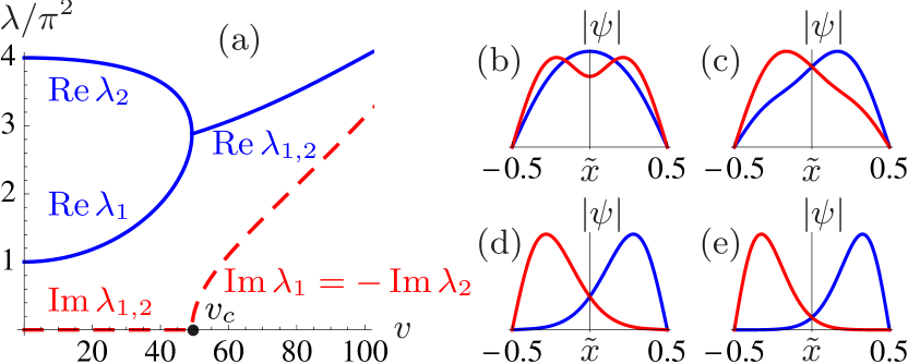
Figure 1: (Color online) (a) Real (solid blue line) and imaginary (dashed red line) parts of the lowest eigenvalues $\lambda_{1,2}(v)$ of the Hamiltonian (5). The spectrum is entirely real until $v=v_{c}\approx 49.25$. (b)–(e) Spatial dependence of the absolute values of the eigenfunctions, $|\psi_{1}({\tilde{x}})|$ (blue) and $|\psi_{2}({\tilde{x}})|$ (red), for $v=0.8\,v_{c}$, $1.2\,v_{c}$, $5\,v_{c}$, and $10\,v_{c}$ respectively.

The Hamiltonian (5) has been recently analyzed in Ref. Rubinstein et al. (2007). It belongs to a class of non-Hermitian Hamiltonians invariant under the combined action of the time-reversal, ${\cal T}$: $f(x)\mapsto f^{*}(x)$, and parity, ${\cal P}$: $f(x)\mapsto f(-x)$, transformations. The $\cal PT$-symmetry of the Hamiltonian (5) ensures that its eigenvalues $\lambda_{n}(v)$ are either real or form complex-conjugated pairs, providing a complex extension of the notion of Hermiticity Bender and Boettcher (1998); Bender (2007). At $v=0$, the spectrum is non-degenerate: $\lambda_{n}(0)=\pi^{2}n^{2}$ ($n=1,2,\dots$). It evolves continuously with $v$ and a nonzero $\mathop{\rm Im}\lambda(v)$ arises only when the two lowest eigenvalues, $\lambda_{1}(v)$ and $\lambda_{2}(v)$, coalesce [see Fig. 1 (a)]. This happens at $v=v_{c}\approx 49.25$ Rubinstein et al. (2007), indicating the transition to a complex-valued spectrum. For $v<v_{c}$, the ground state of (5) is $\cal PT$-symmetric, and hence $|\psi_{1}(\tilde{x})|=|\psi_{1}(-\tilde{x})|$. For $v>v_{c}$, the $\cal PT$-symmetry is spontaneously broken and there is a pair of states with the lowest $\mathop{\rm Re}\lambda(v)$: $\psi_{L}(\tilde{x})=\psi_{1}(\tilde{x})$ and $\psi_{R}(\tilde{x})=\psi_{2}(\tilde{x})=\psi_{1}^{*}(-\tilde{x})$, shifted to the left (right) from the midpoint [see Fig. 1 (b)–(e)].

Spontaneous breaking of the $\cal PT$-symmetry associated with the spectral bifurcation at $v=v_{c}$ explains the appearance of asymmetric superconducting states observed in numerical simulations Vodolazov and Peeters (2007) and recent experiments Vercruyssen et al. (2012). The normal-state instability line, $V_{\text{inst}}(T)$, is specified implicitly by the relation

$$1-T/T_{c0}=(\xi_{0}/L)^{2}\mathop{\rm Re}\lambda_{1}(eV_{\text{inst}}(T)/E_{\text{Th}}),$$ (6)

and exhibits a singular behavior at the critical bias $V_{*}$ given by $eV_{*}=v_{c}E_{\text{Th}}\approx 50E_{\text{Th}}$ (see inset in Fig. 2). The bifurcation of the instability line occurs at the temperature $T_{*}\approx T_{c0}(1-28.44\,\xi_{0}^{2}/L^{2})$. For long wires ($L\gg\xi_{0}$), $T_{*}$ is very close to $T_{c}$.

The time dependence of the emergent superconducting state is determined by $\mathop{\rm Im}\lambda_{1}(v)$. Below the bifurcation threshold, for $V_{\text{inst}}(T)<V_{*}$, the system undergoes at $V=V_{\text{inst}}(T)$ the transition to a stationary superconducting state, with the superconducting chemical potential being the half-sum of the chemical potentials in the terminals. This state is supercurrent-carrying, and can withstand a maximum phase winding of $\pi$ achieved at the critical bias $V_{*}$. For larger voltages, $V_{\text{inst}}(T)>V_{*}$, two modes, $\psi_{L}(x)$ and $\psi_{R}(x)$, nucleate simultaneously at $V_{\text{inst}}(T)$. The resulting bimodal superconducting state is non-stationary since the left and right modes feel different electrochemical potentials and their phases rotate with opposite frequencies, $\Omega_{L,R}(V)=\mp E_{\text{Th}}\mathop{\rm Im}\lambda_{1}(eV/T)$. This will result in the Josephson generation with the differential frequency $\Omega(V)=\Omega_{R}(V)-\Omega_{L}(V)\propto\sqrt{V-V_{*}}$ as $V_{\text{inst}}(T)\to V_{*}$. Though these supercurrent oscillations are locked to the superconducting part they may excite oscillations of the normal current in the whole circuit. Thus the dc biased NSN microbridge may act as a voltage-tunable generator of an ac current, with the maximal amplitude of oscillations expected in the coherent regime, $V-V_{*}\sim V_{*}$. The possibility of experimental observation of such a generation remains an open problem.

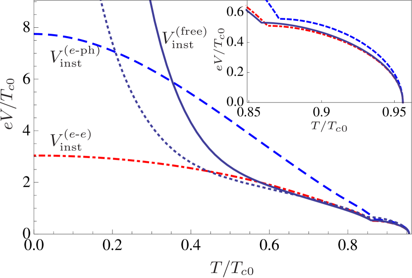
Figure 2: (Color online) Instability voltage as a function of temperature, $V_{\text{inst}}(T)$, obtained numerically for a wire of length $L=15\xi_{0}$ for three limiting types of the distribution function: without inelastic relaxation (solid blue line), and with dominant $e$-$e$ (dot-dashed line) or $e$-ph (dashed line) relaxation. Dotted curve illustrates the suppression of $V_{\text{inst}}^{\text{(free)}}(T)$ by a finite terminal resistance, $\beta=0.1$ (see text). Inset shows the behavior in the vicinity of the bifurcation point $eV_{*}\approx 50E_{\text{Th}}\approx 0.57\,T_{c0}$.

Incoherent regime.—As the voltage is increased far above the bifurcation threshold, $V_{\text{inst}}(T)\gg V_{*}$, the eigenmodes $\psi_{L,R}(x)$ gradually localize near the corresponding terminals, with their size, $a(V)$, becoming much smaller then the wire length [see Fig. 1 (b)–(e)]. This is the incoherent regime, where the overlap between $\psi_{L}(x)$ and $\psi_{R}(x)$ is exponentially small, supercurrent oscillations are suppressed, and nucleation of superconductivity near each terminal can be described independently Vercruyssen et al. (2012).

Using $a(V)/L$ as a small parameter and still working in the vicinity of $T_{c}$, we linearize $F(E,x)$ near the left terminal and reduce Eq. (1) to the form: $(L^{R}_{\omega})^{-1}=i\pi(\omega+eV)/8T-\ln(T/T_{c0})-{\cal H}_{\alpha}$, where the operator

$${\cal H}_{\alpha}=-\xi_{0}^{2}\partial_{x_{L}}^{2}+\alpha x_{L},\qquad x_{L}\geq 0,$$ (7)

acts on the semiaxis $x_{L}\equiv x+L/2\geq 0$ with the boundary condition $\psi(0)=0$. The complex parameter $\alpha$ is a functional of the distribution function:

$$\alpha\Bigl{(}\frac{eV}{T}\Bigr{)}=-\int\frac{dE\,\partial_{x}F(E-eV/2,x)|_{x=-L/2+a(V)}}{2(E-i0)}.$$ (8)

The ground state of the Hamiltonian (7) has the energy $\gamma_{0}(\alpha\xi_{0})^{2/3}$ and the wave function $\psi_{0}(x_{L})=\mathop{\rm Ai}(x_{L}/a-\gamma_{0})/\sqrt{a}\mathop{\rm Ai}^{\prime}(-\gamma_{0})$, where $-\gamma_{0}\approx-2.34$ is the first zero of the Airy function, and $a=(\xi_{0}^{2}/\alpha)^{1/3}$ is the nucleus size Ivlev and Kopnin (1984). For the instability line we get:

$$1-T/T_{c0}=\gamma_{0}\xi_{0}^{2/3}\mathop{\rm Re}\alpha^{2/3}(eV_{\text{inst}}(T)/T).$$ (9)

The left and right unstable states rotate with the frequencies $\Omega_{L,R}(V)=\mp[eV-\Omega_{1}(V)]$, where $\Omega_{1}(V)=(8T_{c0}/\pi)\gamma_{0}\xi_{0}^{2/3}\mathop{\rm Im}\alpha^{2/3}(eV/T)$ is a small correction to the Josephson frequency determined by the electrochemical potential of the corresponding terminal. At the instability line, $V=V_{\text{inst}}(T)$, the size $a$ of the unstable mode is of the order of the temperature-dependent superconducting coherence length $\xi(T)\sim(1-T/T_{c0})^{-1/2}\xi_{0}$.

For long wires ($L\gg\xi_{0}$), the incoherent regime partly overlaps with the weak-nonequilibrium regime. Then for $eV_{*}\ll eV_{\text{inst}}(T)\ll T_{c}$, Eq. (9) gives a universal answer

$$\frac{eV_{\text{inst}}(T)}{T_{c0}}=\frac{2^{7/2}}{\pi}\frac{L}{\xi_{0}}\left(\frac{T_{c0}-T}{\gamma_{0}T_{c0}}\right)^{3/2},$$ (10)

which could have also been deduced from Eq. (6) using the quasiclassical approximation for $\lambda_{1}(v)$ at $v\gg 1$. Equation (9) exactly coincides with the result of Ref. Ivlev and Kopnin (1984), predicting that superconductivity nucleates near the terminals at a finite current $I_{\text{inst}}(T)\approx 0.356\,I_{c}(T)$.

The position of the instability line in the incoherent regime at large biases, $eV_{\text{inst}}(T)\gg T_{c}$, depends on the relation between the inelastic lengths $l_{\text{\emph{e-e}}}$ and $l_{\text{\emph{e}-ph}}$, the wire length $L$, and the nucleus size $a(V)$. The presence of the latter scale, which probes the distribution function near the boundaries of the wire, leads to a rich variety of regimes realized at different temperatures.

For the three limiting distributions [Eqs. (3) and (4)], the function $\alpha(u)$ can be found analytically: (i) $\alpha_{\text{free}}(u)=[\psi(1/2+iu/2\pi)-\psi(1/2)]/L$ for the non-interacting case, $L\ll l_{\text{\emph{e-e}}},l_{\text{\emph{e}-ph}}$, where $\psi(x)$ is the digamma function; (ii) $\alpha_{\text{\emph{e}-ph}}(u)=i\pi u/4L$ for strong lattice thermalization, $l_{\text{\emph{e}-ph}}\ll a(V)\ll L\ll l_{\text{\emph{e-e}}}$; and (iii) $\alpha_{\text{\emph{e-e}}}(u)=[i\pi u/4+3u^{2}/2\pi^{2}]/L$ for the dominant $e$-$e$ interaction, $l_{\text{\emph{e-e}}}\ll a(V)\ll L\ll l_{\text{\emph{e}-ph}}$. In case (ii), the instability line $V_{\text{inst}}^{\text{$e$-ph}}(T)$ is given by Eq. (10). In the vicinity of $T_{c}$, the instability lines in cases (i) and (iii) are given by:

$$\frac{eV_{\text{inst}}^{\text{(free)}}(T)}{T_{c0}}=1.13\exp\left\{\frac{L}{\xi_{0}}\left(\frac{T_{c0}-T}{\gamma_{0}T_{c0}}\right)^{3/2}\right\},$$ (11)

$$\frac{eV_{\text{inst}}^{\text{($e$-$e$)}}(T)}{T_{c0}}=\left(\frac{2\pi^{2}}{3}\frac{L}{\xi_{0}}\right)^{1/2}\left(\frac{T_{c0}-T}{\gamma_{0}T_{c0}}\right)^{3/4}.$$ (12)

Counterintuitively, in cases (i) and (iii) the instability current $I_{\text{inst}}(T)\propto V_{\text{inst}}(T)/L$ has a nontrivial dependence on the system size, as opposed to Eq. (10). Such a behavior is a consequence of strong nonequilibrium in the wire. The limiting curves $V_{\text{inst}}^{\text{(free)}}(T)$, $V_{\text{inst}}^{\text{($e$-ph)}}(T)$, and $V_{\text{inst}}^{\text{($e$-$e$)}}(T)$ for all temperatures obtained numerically from Eq. (1) for the wire with $L/\xi_{0}=15$ are shown in Fig. 2. The universal behavior at small biases can be easily seen (inset). Since the ratio $L/\xi_{0}$ is not very large, the instability line becomes strongly dependent on the distribution function already for $V\gtrsim V_{*}$.

The most exciting feature of our results is the exponential growth of $V_{\text{inst}}(T)$ with decreasing temperature in the non-interacting case, Eq. (11). Hence, even a small deviation of the distribution function from the two-step form (3) will drastically modify $V_{\text{inst}}(T)$. As an example, consider the effect of a finite resistance of the normal terminals. Then the function $F_{L}(E)$ in Eq. (3) will be replaced by $F_{L}(E)=\beta F_{0}(E+eV/2)+(1-\beta)F_{0}(E-eV/2)$, where $V$ is the voltage applied to the NSN microbridge, and $\beta=R_{T}/(R_{N}+2R_{T})$ [$R_{T}$ and $R_{N}$ are the resistances of the N and S part of the junction, respectively]. The resulting $V_{\text{inst}}(T)$ for $\beta=0.1$ is shown by the dotted blue line in Fig. 2. While $V_{\text{inst}}(T)$ is unchanged for small biases, it is strongly suppressed compared to $V_{\text{inst}}^{\text{(free)}}(T)$ for large biases.

Low-temperature behavior.—The exponential growth of $V_{\text{inst}}^{\text{(free)}}(T)$ in the non-interacting case formally implies that superconductivity at $T=0$ might persist up to exponentially large voltages, $\ln(eV_{\text{inst}}(0)/T_{c0})\sim L/\xi_{0}\gg 1$. This conclusion is wrong, since inelastic relaxation and heating become important with increasing $V$, even if they were negligible at $V=0$. To study the low-$T$ part of the instability line, we consider here a model of the e-ph interaction (e-e relaxation neglected) when the phonon temperature is assumed to coincide with the base temperature of the terminals and e-ph relaxation is weak at $T_{c}$: $l_{\text{\emph{e}-ph}}(T_{c})\gg L$ (as in the experiment Vercruyssen et al. (2012)).

With decreasing $T$ below $T_{c}$, the instability line first follows Eq. (11). At the same time, $l_{\text{\emph{e}-ph}}$ decreases and eventually the distribution function in the middle of the wire becomes nearly thermal with the effective temperature $T_{\text{eff}}$. This happens when $T_{\text{eff}}$ obtained from the heat balance equation Giazotto et al. (2006), $(eV/L)^{2}\sim T_{\text{eff}}^{5}/T_{c}^{3}l_{\text{\emph{e}-ph}}^{2}(T_{c})$, becomes so large that $l_{\text{\emph{e}-ph}}(T_{\text{eff}})\sim L$. The corresponding voltage, $V_{\text{ph}}$, can be estimated as $eV_{\text{ph}}/T_{c}\sim[l_{\text{\emph{e}-ph}}(T_{c})/L]^{2/3}$. Consequently, the exponential growth (11) persists for voltages $V_{*}\lesssim V\lesssim V_{\text{ph}}$, corresponding to the temperature range $T_{\text{ph}}\lesssim T\lesssim T_{*}$, where with logarithmic accuracy $1-T_{\text{ph}}/T_{c0}\sim(\xi_{0}/L)^{2/3}$.

For higher biases, $V>V_{\text{ph}}$, electrons in the central part of the wire have the temperature $T_{\text{eff}}$. However, the parameter $\alpha$, Eq. (8), is determined by the distribution function in the vicinity of the terminals which is not thermal. Matching solution of the collisionless kinetic equation for $0<x_{L}<l_{\text{\emph{e}-ph}}(T_{\text{eff}})$ at the effective right “boundary”, $x_{L}=l_{\text{\emph{e}-ph}}(T_{\text{eff}})$, with the function (4) with $T(x)=T_{\text{eff}}$, we obtain $\alpha\sim 1/l_{\text{\emph{e}-ph}}(T_{\text{eff}})$. Therefore, for $V\gtrsim V_{\text{ph}}$ we get with logarithmic accuracy:

$$\frac{eV_{\text{inst}}(T)}{T_{c0}}\sim\frac{L}{\xi_{0}}\left(\frac{l_{\text{\emph{e}-ph}}(T_{c})}{\xi_{0}}\right)^{2/3}\left(\frac{T_{c0}-T}{T_{c0}}\right)^{5/2}.$$ (13)

Equation (13) corresponding to the case $a(V)\ll l_{\text{\emph{e}-ph}}\ll L$ is different from the expression (10) when phonons are important already at $T_{c}$, and $l_{\text{\emph{e}-ph}}\ll a(V)\ll L$. The scaling dependence of Eq. (13) on $L$ indicates that the stability of the normal state is controlled by the applied current, similar to Eq. (10). At zero temperature the instability current exceeds the thermodynamic depairing current by the factor of $(l_{\text{\emph{e}-ph}}(T_{c})/\xi_{0})^{2/3}\gg 1$.

Discussion.—Our general procedure locates the absolute instability line, $V_{\text{inst}}(T)$, of the normal state for a voltage-biased NSN microbridge. Following experimental data Vercruyssen et al. (2012) we assumed that the onset of superconductivity is of the second order. While non-linear terms in the TDGL equation are required to determine the order of the phase transition Serbyn and Skvortsov , we note that were it of the first order, its position would be shifted to voltages higher than $V_{\text{inst}}(T)$.

In the vicinity of $T_{c}$, the problem of finding $V_{\text{inst}}(T)$ can be mapped onto a one-dimensional quantum mechanics in some potential $U(x)$. For small biases, $eV\ll T_{c0}$, the potential $U(x)$ does not depend on the distribution function details, explaining universality of the instability line, including the bifurcation from the single-mode to the bimodal superconducting state at $eV\sim 50E_{\text{Th}}$ Rubinstein et al. (2007) and nucleation of superconductivity in the vicinity of the terminals for larger biases Ivlev and Kopnin (1984).

For $eV\gtrsim T_{c0}$, the potential $U(x)$ becomes a functional of the normal-state distribution function, producing $V_{\text{inst}}(T)$ that is strongly sensitive to inelastic relaxation mechanisms in the wire. For the dominant $e$-ph interaction, the instability is controlled by the electric field ${\cal E}=V/L$ [Eqs. (10) and (13)], while in the opposite case [Eqs. (11) and (12)], the instability cannot be solely interpreted as current or voltage-driven. At zero temperature, the (nonuniform) superconducting state can withstand a current which is parametrically larger than the thermodynamic depairing current.

High sensitivity of $V_{\text{inst}}(T)$ to the details of the distribution function opens avenues for its use as a probe of inelastic relaxation in the normal state. The shape of $V_{\text{inst}}(T)$ can be further used to determine the dominating relaxation mechanism and extract the corresponding inelastic scattering rate.

We are grateful to M. V. Feigel’man, A. Kamenev, T. M. Klapwijk, J. P. Pekola, V. V. Ryazanov, J. C. W. Song, and D. Y. Vodolazov for discussions. This work was partially supported by the Russian Federal Agency of Education (contract No. P799) (M. A. S.).

References

- Kopnin (2001) N. B. Kopnin, Theory of Nonequilibrium Superconductivity (Oxford University Press, New York, 2001).
- Gray (1981) K. Gray, ed., Nonequilibrium superconductivity, phonons, and Kapitza boundaries (Plenum Press, New York, 1981).
- Gulian and Zharkov (1999) A. Gulian and G. Zharkov, Nonequilibrium Electrons and Phonons in Superconductors, Selected Topics in Superconductivity (Springer, 1999).
- Langenberg and Larkin (1986) D. Langenberg and A. Larkin, Nonequilibrium superconductivity, Modern problems in condensed matter sciences (North-Holland, 1986).
- Vodolazov et al. (2003) D. Y. Vodolazov, F. M. Peeters, L. Piraux, S. Mátéfi-Tempfli, and S. Michotte, Phys. Rev. Lett. 91, 157001 (2003).
- Xiong et al. (1997) P. Xiong, A. V. Herzog, and R. C. Dynes, Phys. Rev. Lett. 78, 927 (1997).
- Rogachev et al. (2006) A. Rogachev, T.-C. Wei, D. Pekker, A. T. Bollinger, P. M. Goldbart, and A. Bezryadin, Phys. Rev. Lett. 97, 137001 (2006).
- Li et al. (2011) P. Li, P. M. Wu, Y. Bomze, I. V. Borzenets, G. Finkelstein, and A. M. Chang, Phys. Rev. B 84, 184508 (2011).
- Astafiev et al. (2012) O. V. Astafiev, L. B. Ioffe, S. Kafanov, Y. A. Pashkin, K. Y. Arutyunov, D. Shahar, O. Cohen, and J. S. Tsai, Nature 484, 355 (2012).
- Ivlev and Kopnin (1984) B. I. Ivlev and N. B. Kopnin, Adv. Phys. 33, 47 (1984).
- Meyer and Minnigerode (1972) J. Meyer and G. Minnigerode, Physics Letters A 38, 529 (1972).
- Langer and Ambegaokar (1967) J. S. Langer and V. Ambegaokar, Phys. Rev. 164, 498 (1967).
- McCumber and Halperin (1970) D. E. McCumber and B. I. Halperin, Phys. Rev. B 1, 1054 (1970).
- Keizer et al. (2006) R. S. Keizer, M. G. Flokstra, J. Aarts, and T. M. Klapwijk, Phys. Rev. Lett. 96, 147002 (2006).
- Vercruyssen et al. (2012) N. Vercruyssen, T. G. A. Verhagen, M. G. Flokstra, J. P. Pekola, and T. M. Klapwijk, Phys. Rev. B 85, 224503 (2012).
- Snyman and Nazarov (2009) I. Snyman and Y. V. Nazarov, Phys. Rev. B 79, 014510 (2009).
- Gorkov and Eliashberg (1968) L. P. Gorkov and G. M. Eliashberg, Sov. Phys. JETP 27, 328 (1968).
- Kramer and Watts-Tobin (1978) L. Kramer and R. J. Watts-Tobin, Phys. Rev. Lett. 40, 1041 (1978).
- Michotte et al. (2004) S. Michotte, S. Mátéfi-Tempfli, L. Piraux, D. Y. Vodolazov, and F. M. Peeters, Phys. Rev. B 69, 094512 (2004).
- Vodolazov (2007) D. Y. Vodolazov, Phys. Rev. B 75, 184517 (2007).
- Elmurodov et al. (2008) A. K. Elmurodov, F. M. Peeters, D. Y. Vodolazov, S. Michotte, S. Adam, F. d. M. de Horne, L. Piraux, D. Lucot, and D. Mailly, Phys. Rev. B 78, 214519 (2008).
- Rubinstein et al. (2007) J. Rubinstein, P. Sternberg, and Q. Ma, Phys. Rev. Lett. 99, 167003 (2007).
- Chtchelkatchev and Vinokur (2009) N. Chtchelkatchev and V. Vinokur, Europhys. Lett. 88, 47001 (2009).
- Giazotto et al. (2006) F. Giazotto, T. T. Heikkilä, A. Luukanen, A. M. Savin, and J. P. Pekola, Rev. Mod. Phys. 78, 217 (2006).
- Chen et al. (2009) Y. Chen, S. D. Snyder, and A. M. Goldman, Phys. Rev. Lett. 103, 127002 (2009).
- Tian et al. (2005) M. Tian, N. Kumar, S. Xu, J. Wang, J. S. Kurtz, and M. H. W. Chan, Phys. Rev. Lett. 95, 076802 (2005).
- Boogaard et al. (2004) G. R. Boogaard, A. H. Verbruggen, W. Belzig, and T. M. Klapwijk, Phys. Rev. B 69, 220503 (2004).
- Larkin and Varlamov (2002) A. I. Larkin and A. A. Varlamov, Theory of Fluctuations in Superconductors (Oxford University Press, New York, 2002).
- Levchenko and Kamenev (2007) A. Levchenko and A. Kamenev, Phys. Rev. B 76, 094518 (2007).
- Feigel’man et al. (2000) M. V. Feigel’man, A. I. Larkin, and M. A. Skvortsov, Phys. Rev. B 61, 12361 (2000).
- Kamenev (2011) A. Kamenev, Field Theory of Non-Equilibrium Systems (Cambridge University Press, 2011).
- Nagaev (1995) K. E. Nagaev, Phys. Rev. B 52, 4740 (1995).
- Pothier et al. (1997) H. Pothier, S. Guéron, N. O. Birge, D. Esteve, and M. H. Devoret, Phys. Rev. Lett. 79, 3490 (1997).
- Bender and Boettcher (1998) C. M. Bender and S. Boettcher, Phys. Rev. Lett. 80, 5243 (1998).
- Bender (2007) C. M. Bender, Rep. Prog. Phys. 70, 947 (2007).
- Vodolazov and Peeters (2007) D. Y. Vodolazov and F. M. Peeters, Phys. Rev. B 75, 104515 (2007).
- (37) M. Serbyn and M. A. Skvortsov, in preparation.