On the Diversity and Complexity of Absorption Line Profiles Produced by Outflows in Active Galactic Nuclei

Abstract

Understanding the origin of AGN absorption line profiles and their diversity could help to explain the physical structure of the accretion flow, and also to assess the impact of accretion on the evolution of the AGN host galaxies. Here we present our first attempt to systematically address the issue of the origin of the complexities observed in absorption profiles. Using a simple method, we compute absorption line profiles against a continuum point source for several simulations of accretion disk winds. We investigate the geometrical, ionization, and dynamical effects on the absorption line shapes. We find that significant complexity and diversity of the absorption line profile shapes can be produced by the non-monotonic distribution of the wind velocity, density, and ionization state. Non-monotonic distributions of such quantities are present even in steady-state, smooth disk winds, and naturally lead to the formation of multiple and detached absorption troughs. These results demonstrate that the part of a wind where an absorption line is formed is not representative of the entire wind. Thus, the information contained in the absorption line is incomplete if not even insufficient to well estimate gross properties of the wind such as the total mass and energy fluxes. In addition, the highly dynamical nature of certain portions of disk winds can have important effects on the estimates of the wind properties. For example, the mass outflow rates can be off up to two orders of magnitude with respect to estimates based on a spherically symmetric, homogeneous, constant velocity wind.

1. INTRODUCTION

Accretion disk winds are among the most promising physical mechanisms able to link the small and the large scale phenomena in active galactic nuclei (AGN) and to shed light on the physics of mass accretion/ejection around supermassive black holes (SMBHs). Such winds are currently directly observed, as blueshifted and broadened absorption lines in the UV and X-ray spectra of a substantial fraction of AGN (e.g., Crenshaw et al., 2003).

In the UV band we observe, with decreasing width of the absorption troughs, broad absorption lines (BALs) in about 15 % of optically selected AGN (e.g., Knigge et al., 2008; Gibson et al., 2009); mini-broad absorption lines (mini-BALs) and narrow absorption lines (NALs) in about 30 % of AGN (Ganguly & Brotherton, 2008). Once corrected for selection effects, the intrinsic fraction of AGN hosting BALs is estimated to be $\sim 30-40$ % (Allen et al., 2011); summing also the corrected fraction for mini-BALs and NALs, the intrinsic fraction of AGN hosting blueshifted UV absorption lines results to be as high as $\sim 70$ % (Hamann et al., 2012). In all these cases, the absorbers are associated to resonant transitions of moderately ionized elements like Mg ii, Al iii, C iv, Si v, and can be outflowing with velocities as high as $\sim 0.2$ $c$, the main difference among them being in the width of their absorption troughs. Given their large width, BAL structures are the easiest to be identified even in low-resolution UV spectra, and have therefore been studied in much more detail than mini-BAL and NAL structures. The shape of BAL troughs is quite complex, showing a variety of profiles among different sources (e.g., Turnshek, 1984; Foltz et al., 1987; Turnshek et al., 1988; Hall et al., 2002). When high spectral resolution, high signal-to-noise observations have become available, generally also mini-BALs and NALs showed a variety of profiles (e.g., Misawa et al., 2007; Wu et al., 2010; Hamann et al., 2011; Rodríguez Hidalgo et al., 2011). Recently a number of AGN have been shown to display strong variability in their UV absorption troughs, including emergence of BAL structures and transitions from mini-BALs to BALs (e.g., Ma, 2002; Hamann et al., 2008; Leighly et al., 2009; Krongold et al., 2010; Vivek et al., 2012).

In the X-ray spectra of $\sim 50$ % of AGN, we observe also lower-velocity (from $\sim 100$ to $\sim 1000$ km s^-1) outflowing ionized gas (the so-called warm absorber) in the transitions of ionized elements such as C vi, O vii, O viii, Si vi (e.g., McKernan et al., 2007). Higher velocity absorbing gas in the transitions of Fe xxv and Fe xxvi, with blueshift in the range $0.003-0.3$ $c$ is observed in a number of AGN (e.g., Pounds et al., 2003; Risaliti et al., 2005; Cappi, 2006; Miniutti et al., 2007; Turner et al., 2008; Giustini et al., 2011); their fraction among the AGN population is currently unknown, the only reliable estimate being of about $30-40$ % for a sample of low redshift AGN (Tombesi et al., 2010). X-ray BALs outflowing up to $0.7$ $c$ have been also observed in a handful of AGN (Chartas et al., 2002, 2003, 2009; Lanzuisi et al., 2012). The ionization state of the X-ray absorbers spans a large range of values, from e.g. C vi in the case of warm absorbers up to Fe xxvi for X-ray BALs. The observed high-velocity X-ray absorbers profiles are quite complex and display strong temporal variability both in depth and velocity shift; also for the case of the lower-velocity X-ray warm absorbers, deep observations have revealed significant complexities in the absorption trough profiles (e.g., Ramírez et al., 2005; Pounds & Vaughan, 2011) and variability in ionization and velocity shift (e.g., see Longinotti et al., 2010; Matt et al., 2011, for some recent results).

Velocity and ionization state are only two of the physical properties of AGN winds; the mass and energy fluxes carried by them are other fundamental properties that we wish to be able to measure in order to quantify the actual impact of these winds on the surrounding environment, i.e., the amount of feedback. To measure the mass and energy flux, the density of the wind material and the distance between the central SMBH and the place where absorption occurs must be known. Unfortunately, these two quantities are difficult to measure, and estimates for them have always relied on several assumptions. In particular, a geometrically and optically thin, constant-density, spherically symmetric, single-zone of gas in ionization equilibrium and outflowing with a uniform velocity has been usually assumed to derive constraints on the distance of the absorbing material from the central ionizing source.

Using these assumptions, reported estimates of the distances of absorbers from the central SMBH range from the inner regions of the accretion disk for the high-velocity X-ray BALs (e.g., Chartas et al., 2009), to the parsec-scale torus for the X-ray warm absorbers (e.g., Blustin et al., 2005), to the kiloparsec-scale for some UV BALs (e.g., Dunn et al., 2010). Currently the uncertainties on the distances are relatively large, which translates to a high uncertainty on the mass outflow rate and on the kinetic energy injection associated with such winds (e.g., Reeves et al., 2003; Krongold et al., 2007; Cappi et al., 2009).

Theoretical arguments and numerical simulations have been used to show that accretion disks are able to launch and accelerate powerful outflows by various physical mechanisms such as radiation pressure, magnetic pressure, and thermal pressure (see e.g. Königl, 2006; Proga, 2007; Everett, 2007, for reviews on the subject). The driving mechanism and the accreting system physical parameters (e.g., accretion rate, black hole mass, magnetic field configuration, UV/X-ray flux ratio) determine the wind characteristics (e.g., Proga, 2005). Despite the many parameters that combine themselves in complicated ways, only a few geometries of streamlines are shown by AGN accretion disk wind models.

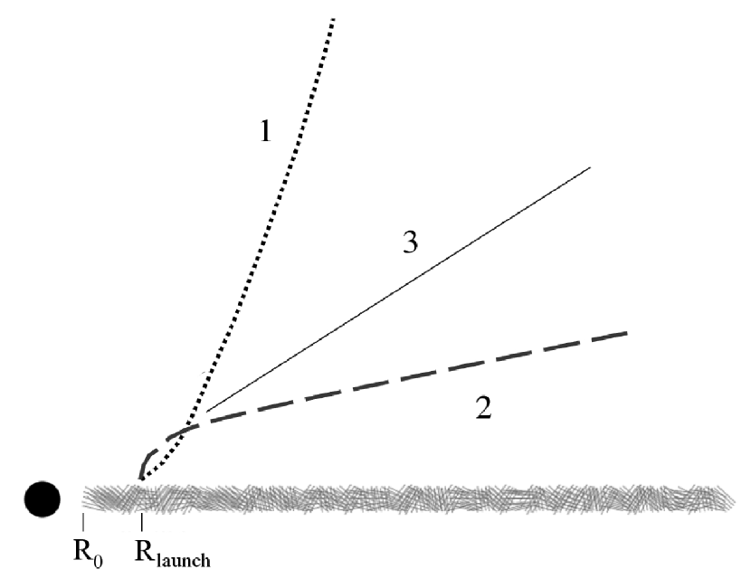
Figure 1.— The three “typical” streamlines for accretion disk winds. 1: MHD-typical, polar and convex streamline. 2: hydrodynamical-typical, equatorial and concave streamline. 3: a radial streamline typical of spherically symmetric winds.

Figure 1 shows the main general shapes of streamlines that are predicted by models of AGN accretion disk winds. Number 1 is a convex, polar streamline, typical of magnetic driving scenarios (e.g., Blandford & Payne, 1982; Lovelace et al., 1991; Krasnopolsky et al., 2003; Anderson et al., 2005; Everett, 2005). Number 2 is a concave, more equatorial streamline, typical of line-driven (e.g., Proga et al., 2000; Proga & Kallman, 2004) and thermally driven disk winds (e.g., Woods et al., 1996; Font et al., 2004; Luketic et al., 2010). What is usually assumed in order to deduce quantities such as mass outflow rate, ionization state, or absorber distance from the continuum source is the configuration number 3, i.e. a radial flow.

However, the different geometries correspond to very different wind properties: the mass flux $\dot{m}_{out}$ across the area of a flow tube, $A(r)$ is

$$\dot{m}_{out}=A(r)\upsilon(r)\rho(r)$$ (1)

where $\upsilon$ is the velocity normal to the area, and $\rho$ is the density. For a simple radial wind with a constant velocity, $A(r)\propto r^{2}$ and $\rho(r)\propto r^{-2}$, whereas for a cylindrical wind (with constant velocity) $A(r)=const$ and $\rho(r)=const$. This density dependence on the flow geometry has received little consideration in previous works on estimating the flow mass and energy rates using observations (however, see Waters & Proga, 2012).

In this article we will report on results from our first attempt of systematically addressing the following questions: what drives the appearance of different line profiles? Can we distinguish among different geometries for accretion disk winds from observations? How reliable are estimates of wind properties, when a radial or spherical flow is assumed? The secondary questions that will lead to answer the former ones are then: what are the implications of radial flow assumptions when deriving physical quantities related to the wind? Do different wind physical characteristics produce different line profiles? If yes: how and why? Our method to compute line profiles is introduced in Section 2; results are presented in Section 3 and discussed in Section 4; finally, conclusions are presented in Section 5.

2. METHOD

We consider several examples of disk wind models, with an increasing level of completeness or complexity or both. We present results in terms of synthetic absorption line profiles predicted by these models. Specifically, we first consider a simplified, isothermal, thermally driven disk wind model and use steady state solutions as predicted by hydrodynamical simulations similar to those of Font et al. (2004) in Section 3.1; then we consider hydrodynamical simulations as given by Luketic et al. (2010), where the effect of a central X-ray illuminating source is explicitly taken into account, showing the effects of varying ionization state across the flow (Section 3.2); finally we consider the solutions given by Proga & Kallman (2004), showing the effects of the departure of the flow from a steady configuration (Section 3.3).

Our method to compute absorption line profiles adopts a radiation transfer treatment that is simplified to the bare minimum, nonetheless capturing the most important physical and geometrical effects, and as we will show is useful to explore the effects of different wind geometries. Specifically, we ignore scattered radiation and we assume that the continuum photons are emitted by a point source. Therefore we deal with proper “line of sight” (LOS), instead of “cylinder of sight” and line profiles observed at infinity are sensitive only to the radial component of the wind velocity only along a given LOS. This kind of approach is viable for analyzing e.g. X-ray properties of AGN winds because of the compactness of the X-ray source continuum. Having the distributions of the density $\rho$ and the radial velocity $\upsilon_{r}$ for each wind model, we compute synthetic absorption line profiles corresponding to different LOS or equivalently inclination angles. Our procedure is the following: First, we search for resonance points given the continuum frequency, $\nu_{o}$ along a given LOS using the resonance condition

$$\frac{\left(\nu-\nu_{o}\right)}{\nu_{o}}=\frac{\upsilon_{r}}{c}$$ (2)

where $\nu$ is the Doppler shifted flow frequency with respect to the continuum, and $\upsilon_{r}$ is the velocity along the LOS. We then use the Sobolev approximation to compute the optical depth:

$$\tau=\frac{\kappa c}{\nu}\rho\frac{1}{|d\upsilon_{r}(r)/dr|}$$ (3)

where the line opacity $\kappa$ is a product of the oscillator strength and the abundance of a given element and ionization factor for a given ion, and $d\upsilon_{r}(r)/dr$ is the velocity gradient along the LOS (with our approximation it is just the gradient of the radial velocity). To focus on the effects of the density and radial velocity distributions across the flow, we set $\kappa c/\nu=1$ and compute the optical depth $\tau_{\nu,i}$ at a given resonance point $i$, and the total optical depth, $\tau_{\nu}$ at a given frequency by summing up the optical depths at all resonance points that we found

$$\tau_{\nu}=\sum_{i}\tau_{\nu,i}$$ (4)

We finally solve the radiative transfer equation:

$$I=I_{o}e^{-\tau_{\nu}}\rm{.}$$ (5)

Many already studied how synthetic line profiles depend on the wind geometry and viewing angle. However, most of previous studies used kinematic models of accretion disk winds and were applied to cataclysmic variables (e.g., Drew, 1987; Shlosman & Vitello, 1993; Knigge et al., 1995; Long & Knigge, 2002). These models were axisymmetric. They assumed streamlines to be straight lines and the wind velocity to be some prescribed function of the position along the streamline. By varying one of the free parameters (namely the inclination angles that the streamlines made with respect to the disk plane), such models permit the exploration of various wind geometries, but only to some extent. One of the results of these studies is that the formation of blueshifted broad absorption troughs (i.e., P Cygni profiles) can be naturally obtained for a variety of wind geometries. Our work is an extension of those earlier studies as we investigate how the absorption troughs depend on the geometry of the streamlines, the opacity, and the ionization state but instead of using kinematic models we use solutions of hydrodynamical equations obtained by numerical simulations. More sophisticated calculations of wind photoionization and radiative transfer are possible, however they are relatively time consuming and therefore less suitable to the exploration of various geometries (e.g., Sim et al., 2010b).

3. RESULTS

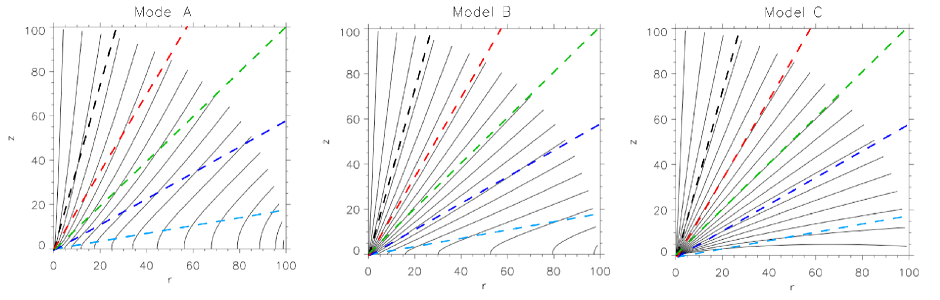
Figure 2.— Streamlines for the three simple isothermal disk wind models adopted from Luketic et al. (2010) (see also Font et al., 2004). The models were computed assuming a density profile at the wind base as the following function of radius, $r_{D}$: $\rho(r)\propto r_{D}^{-\alpha}$ for $\alpha=1.5,2.0,$ and 2.5, from left to right. The colored dashed lines represent the five LOS for which we calculate absorption line profiles: $i=15,30,45,60,$ and 80^∘ for the black, red, green, dark blue, and light blue line, respectively. The length scales on the figure are in units of the radius at which the gas internal energy equals the gravitational energy of the central object located at (0,0).

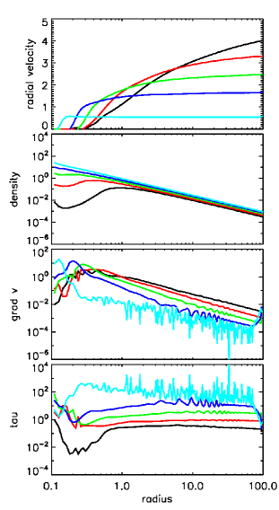
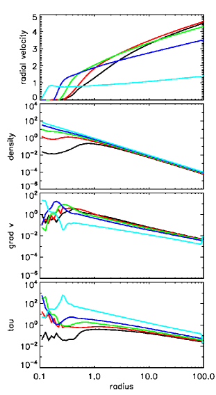
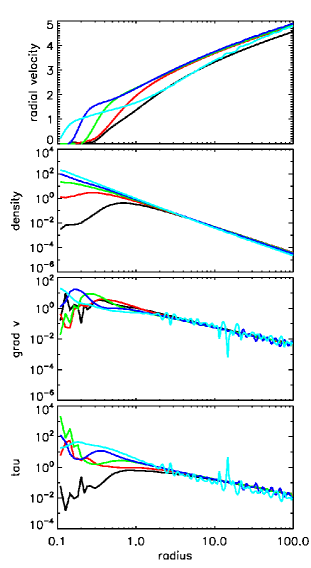
Figure 3.— Radial profiles for the velocity, density, radial velocity gradient, and finally line optical depth, for model A, B, and C from left to right. The color code is as in Figure 2. Radii are in units of the radius at which the gas thermal energy equals the gravitational energy of the central object, while velocities are in units of sound speed.

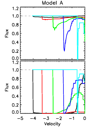
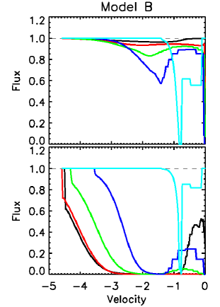
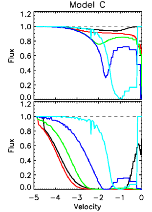
Figure 4.— Absorption line profiles for the for each model, along the five LOS color-coded as in Figure 2. Top panels: profiles computed using the actual opacity of the models; bottom panels: profiles computed increasing the opacity for each LOS until the zero flux level is reached at least in one point in the velocity space.

3.1. Effects of the Overall Wind Geometry

We first consider 2D, axisymmetric, isothermal, steady state disk wind models. We use models computed by Luketic et al. (2010) and refer a reader to this work for details about the simulations. We note that Luketic et al. (2010) performed these simulations to test their code and setup against results presented by Font et al. (2004).

The latter showed that a relatively wide range of the wind geometries and shapes of the streamlines can be modeled by varying the slope of the radial profile of the density along the disk atmosphere (the base of the wind). In particular, Figure 2 shows examples of three different wind geometries assuming a power-law density profile: $\rho(r)\propto r_{D}^{-\alpha}$ and three values of $\alpha$: 1.5 (model A), 2.0 (model B), and $2.5$ (model C). As found by Font et al. (2004), all the three models predict a very similar shape and divergence (i.e., $A(r)$) for the streamlines originating from the inner most part of the disk; for other streamlines (or middle and high inclination angles), some differences and trends among various models start to appear. The flattest radial density profile along the wind base (model A) corresponds to a relatively polar geometry, while the steepest profile (model C) is the one that most resembles the spherical outflow case (quasi radial, with spherical divergence).

We probed the winds along five different LOS, indicated with the colored dashed lines in Fig. 2; the radial velocity, density, radial velocity gradient, and finally optical depth are plotted in Fig. 3 for each model and for each inclination angle. All the quantities are arbitrarily normalized, as at this point, we simply want to explore the qualitative behavior of the different geometries: to this end, what is relevant is the relative contribution of the different parts of the flow and not their absolute magnitude, the latter being strongly dependent on the actual details of the system such as the central mass, the Eddington ratio, and the spectral energy distribution.

Figure 4 shows the resulting absorption line profiles using the same color code as in the previous figures. To show the profile shapes in more detail, the bottom panels of Figure 4 show results where the opacity has been multiplied by a factor so that the point in velocity space where the opacity is maximum reaches the zero flux level for each LOS.

The most obvious difference between the profiles predicted by winds of different geometries is in the shape of the blue wing: very sharp for model A and very smooth for model C. Model B is an intermediate case: similar to model A at high inclination angles ($i\sim 80^{\circ}$), to model C at middle and low inclination angles ($i\lesssim 60^{\circ}$). The main effect of $i$ on the profiles, regardless of the wind model, is on the profile width: the larger the inclination the narrower the profile. However, the profile sensitivity to $i$ is model dependent. In particular, the profile width is most sensitive to $i$ in model A and the least in model C. This is simply a reflection of the fact that model A is polar whereas model C is almost spherically symmetric. The right panels of Figure 3 show that for Model C, at large radii, the flow properties do not depend on $i$ (profiles for various $i$ collapse onto one power-law) as expected for a spherical solution, whereas the panels in the left and middle columns show that the flow properties are strong functions of $i$.

For the highest inclination angle (light blue lines in Figure  3) in Model A and C, the radial profiles for the opacity and the radial velocity gradient appear to be noisy. In the case of Model A, this is a numerical effect which is related to the nearly constant velocity, that makes its gradient very small; as for Model C, the noise reflects the fluctuations in the radial velocity profile close to the base of the wind (i.e. the disk surface).

In this subsection, we consider the isothermal disk wind solutions. One of the key consequences of assuming constant temperature is that the wind velocity along a given streamline is an ever increasing function of the radius. In other words, those models have infinite acceleration zones. This can be seen most clearly in the top right panel of Figure 3 showing the radial velocity for model C and various $i$. In model C, the flow is almost radial so that the velocity plotted in Figure 3 (the radial component) is very similar to the total velocity. Note that this is not the case for the plotted velocity of model A that could give an impression that the velocity saturates at a finite level. This saturation is not caused by a finite acceleration but by projecting the total velocity onto a LOS (in effect, taking only the radial component of the total velocity). This projecting significantly affects the plotted velocity for model A and to some extent for model B.

A more detailed analysis shows that for the case of polar flows (model A), the optical depth is a weak function of radius at large radii. This explains a relatively flat line profiles at large velocities and a sharp edge corresponding to the velocity at $r_{out}$. The flatness of the $\tau$ profile is caused by the relative flatness of the density and radial velocity profiles. In the case of more equatorial flows (model B and C), the density scales as expected for the spherical flow like $r^{-2}$ and $\tau$ is a decreasing function of radius at large radii. Therefore, the line absorption reaches a maximum at some intermediate velocity and then it gradually decreases with increasing velocity with the signature of the finite size of the computational domain (the sharp edge) being weak or undetectable. As we will illustrate in next section, sharp edges or features in the line profiles can be produced not only as artifacts of the finite computational domain but also as physical consequences of the internal structure of the wind (see also the work of Drew, 1987; Shlosman & Vitello, 1993; Knigge et al., 1995).

Although the profile width depends on $i$, its overall shape is not very sensitive to $i$ for these simple isothermal models: the differences between profiles for different wind geometries seen at different inclination angles are not very significant - most profiles are flat, featureless, and differ only in the position of the blue edge. In particular, looking at the bottom panels of Figure 4, it is really hard to distinguish among model B and C, and also among the different inclination angles. For example, the line profile for $i=60^{\circ}$ of model B is very similar to the profile for $i=80^{\circ}$ of model C. Looking at model A, the profile shapes are now undistinguishable among different LOS, the only difference being in the maximum blueshift velocity and the width of the absorption trough. Given the very similar characteristics of the synthetic absorption line profiles resulting from different inclination angles and different geometries, we conclude that different wind geometries are not the main contributors to the very different shapes of observed absorption lines.

3.2. Effects of Finite Acceleration Zone and of Position Dependent Ionization State

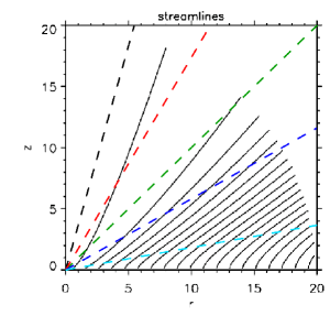
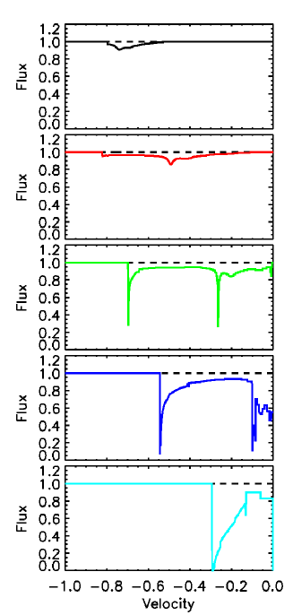
Figure 5.— Top panel: streamlines for the disk wind model of Luketic et al. (2010); bottom panels: absorption line profiles for different inclination angles, with the same color code as in the top panel, for the rerun of the C8 model of Luketic et al. (2010). The velocity scale has been normalized to the maximum outflow velocity $\upsilon_{max}=6.6\times 10^{7}$ cm s^-1.

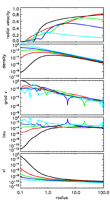
Figure 6.— Radial profiles for the velocity, density, radial velocity gradient, line optical depth, and ionization parameter, for the rerun of the Luketic et al. (2010) model. The color code is as in Figure 5; the quantities have been normalized to their maximum value among all the LOS.

In the previous section, we found that as simple and easy to understand the isothermal models are, they are of a limited usage and could be a source of artifacts in the line profiles. For example, the position of the blue edge in the profile for model A would shift to higher velocities if the outer radius of the computational domain were increased. This shift would be a consequence of the fact that the computation would capture a faster part of the wind solution. For these and other reasons, we consider next a model for which the assumption of isothermal flow was relaxed and instead the gas temperature was computed by introducing physically consistent radiative cooling and heating processes. We use one of the simulations of the thermally driven disk wind from Luketic et al. (2010). Specifically, we use a rerun of their fiducial run (C8) on a grid with an outer radius $r=100r_{C}$, where $r_{C}$ is the Compton radius. For most of their runs, Luketic et al. (2010) used a grid with a smaller outer radius ($r=20r_{C}$). However, to examine and confirm the self-similarity of the flow at large radii, they performed several simulations on the bigger grid. Figure 5 reports the geometry of the wind and the five probed LOS in its top panel, and the corresponding absorption line profiles in its bottom panels. The difference in profiles with respect to the previous case is striking. In this case, the inclination angle $i$ plays a fundamental role in shaping the absorption line profiles. Generally, the profiles are no smooth nor broad anymore, and show two distinct components for a range of $i$.

To associate the line profile characteristics with the wind properties, Fig. 6 shows the radial profiles of the radial velocity, the density, the radial velocity gradient, the optical depth, and the ionization parameter for five $i$’s. The main difference compared to the previous model is that the radial velocity reaches a maximum or two within the computational domain for most $i$ and after reaching the maximum, the radial velocity can significantly decrease with increasing radius (see the top panel of Fig. 6). This results in large velocity gradients and in turn sharp maximums in $\tau$.

However, the line forming region can be smaller than the size of the wind, so that only one of the line components can be produced by a real system. This can occur in winds where changes in the flow ionization limit the formation of a given line to a relatively small region. To illustrate this point, we will scale the ion fraction with the photoionization parameter $\xi=L/4\pi nr^{2}$ where $L$ is the ionizing luminosity, $n$ is the number density of the gas, and $r$ is the distance from the continuum source. Only in special cases $\xi$ is constant, for example when $n\propto r^{-2}$ and the flow is radial and of constant velocity. For a radial flow with variable velocity, $\xi\propto\upsilon(r)$ so $\xi$ increases with increase outflow velocity (e.g., Ramírez et al., 2005). However, for most $i$, in all the disk wind models we discuss here, $n$ decreases with $r$ slower than $r^{-2}$ and could even increase with $r$. Consequently, the photoionization parameter decreases with increasing radius for a given LOS.

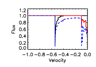
Figure 7.— The effect of varying ionization parameter for the $i=60^{\circ}$ LOS: in black the lower ionization state species, in red the higher ionization state species, in blue dashed line the total line profile without accounting for ionization parameter distribution effects.

In Figure 7, we show the effects of the varying photoionization parameter through the flow, on the absorption line profile for $i=60^{\circ}$. Specifically, we recalculated the profile assuming that the number density of a given species is a function of $\xi$: we used two thresholds with a difference in $\xi$ of about two orders of magnitude (e.g., to mimic the difference between O viii and Fe xxv). The profile without effects of $\xi$ is plotted using a blue dashed line (it is the same profile as in Figure 5 plotted using a blue solid line, and it is double-peaked reflecting the two maxima in the opacity distribution along this LOS visible in Figure 6), while the profiles with the effects of the ionization state are: the red line refers to a highly ionized phase and the black line refers to a lowly ionized one. After taking into account the ionization state distribution across the flow, one can easily lose the double-peakness and find a single absorption trough for each ionic species. Furthermore, as a consequence of the radial distribution of $\xi$ through the flow, one can have a greater blueshift for the lowly ionized species than for the highly ionized ones. This is an opposite trend to the one expected for a radial outflow!

Under the assumption of a simple radial flow, to explain the presence of multiple absorption line profiles that display complexities both in the velocity and ionization state parameter spaces, one typically is pressed to invoke a multiple-phase absorbing gas at different locations and with different velocities. However, by relaxing the radial flow assumption and adopting a more realistic scenario, these complexities are natural consequences of the geometrical extent of the outflow and proper treatment of cooling/heating processes.

3.3. Effects of Unsteady Behavior

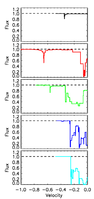
Figure 8.— Blueshifted absorption line profiles computed for the LD accretion disk wind model of Proga & Kallman (2004) as seen by the different inclination angles $i=$ 60, 65, 70, 75, and 80^∘ from the disk rotational axis for the black, red, green, blue, and light blue, respectively. The velocity scale has been normalized to the maximum outflow velocity $\upsilon_{max}=2.9\times 10^{9}$ cm s^-1.

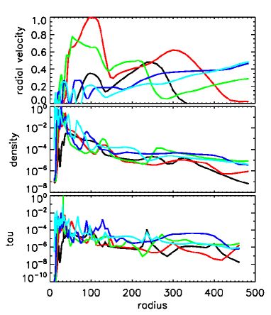
Figure 9.— From top to bottom velocity, density, and optical depth profiles as a function of radius, for the same inclination angles color coded in Figure 8. The radius in in units of the inner disk radius, $R_{0}=3R_{S}$ where $R_{S}=2GM_{BH}/c^{2}$ is the Schwarzschild radius (see Proga & Kallman, 2004, for details).

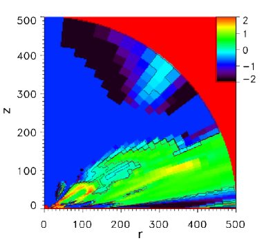
Figure 10.— Map of the ratio between the mass outflow rate computed under the spherical symmetry assumption, and by using actual values from the numerical simulations of Proga & Kallman (2004). The axes are in units of the inner disk radius, $R_{0}=3R_{S}$ where $R_{S}=2GM_{BH}/c^{2}$ is the Schwarzschild radius.

So far, we have considered time-independent solutions of disk wind models. To illustrate the effects of unsteady solutions, we refer to the line-driven (LD) accretion disk wind model as presented by Proga & Kallman (2004). These authors presented hydrodynamical simulations of a quasar, demonstrating how the accreting system is able to launch powerful equatorial disk winds. In particular, they found three different regimes for the flow: a ’hot flow’ in the polar region, where the density and the velocity are very low; a ’fast stream’ in the equatorial region, where a wind successfully developes, and a ’transitional zone’ in between the two, where the flow is hot and struggles to escape the system. The ’transitional zone’ is effectively shielding the ’fast stream’ flow from the strong central ionizing continuum, preventing it from becoming over-ionized and losing acceleration in the UV resonant absorption lines. Broad-band X-ray spectra computed using detailed Monte Carlo simulations to treat the radiative transfer in the flow are presented in Sim et al. (2010b). Here we limit our study to the analysis of simple absorption profiles computed under the Sobolev approximation as in the previous Sections, using as input the flow physical parameters as given by the Proga & Kallman (2004) hydrodynamical simulations.

In Figure 8, we show the absorption line profiles computed for five different inclination angles through the ’fast stream’ and the ’transitional zone’ of the flow, $i=60,65,70,75,$ and $80^{\circ}$ from top to bottom. Figure 9 shows the radial profiles of the velocity, density, and optical depth for the same inclination angles as above. What is immediately clear is the departure from the spherical symmetry: both the radial velocity and the density are not monotonic. Interesting physical insights can be obtained when looking at the $65^{\circ}$ and $70^{\circ}$ LOS, that are the red and green lines in Figure 8 and Figure 9. These two inclination angles roughly correspond to the transitional zone from the slow to the fast stream zone. Observationally, the $65^{\circ}$ red spectral line profile shows much more blueshifted absorption than the $70^{\circ}$ green profile. However, when looking at the radial velocity plot in Figure 9, it can be seen that the absorption at high velocity for $i=65^{\circ}$ happens close to the origin ($R\sim 150R_{0}$, where $R_{0}=8.8\times 10^{13}$ cm is the inner radius of the accretion disk and is equal to 3 Schwarzschild radii), where the dynamical instabilities of the transitional zone of the wind are the highest. At larger radii, for $i=65^{\circ}$, the radial velocity decreases: the deep absorption signature at $\upsilon_{out}\sim 0.65\upsilon_{max}$ is due to a portion of the wind (a ’puff’, a blob) that will shortly (on dynamical time scale) fall back toward the disk plane. On the other hand, for $i=70^{\circ}$, the maximum of the absorption is reached at much lower velocities, and shapes a broad deep trough at $\upsilon_{out}\sim 0.1-0.3\upsilon_{max}$. One can see that most of this absorption happens at large radii, $R\sim 300R_{0}$ , and that this portion of the wind is more stable and effectively accelerated to leave the computational domain.

Among the the considered LOS for this particular model, only the largest inclination angles (70, 75, and 80^∘) track portions of the flow that will successfully escape the system, albeit they show the less blueshifted absorption profiles (Figure 8). On the contrary, the highly-blueshifted profile associated to the 65^∘ tracks a part of the flow where the gas is initially accelerated to the highest velocities, but being so close to the central continuum source it becomes quickly over-ionized, so loses driving force, and falls back to the disk plane. This lack of one-to-one correspondency between blueshift and terminal velocity of the wind is again contrary to the expectations of a simple radial flow of constant velocity. Dynamical effects can be extremely important in shaping the appearance of absorption line profiles, and should be taken into account when deriving physical properties such as mass and energy fluxes associated to the wind.

All these considerations can be also visualized in Figure 10, that shows the map of the ratio between the outflow mass flux computed under the spherical symmetric assumption and the actual outflow mass flux. The strong blueshifted absorption seen along the $i=65^{\circ}$ LOS corresponds to the structure close to the origin, where the mass loss rate estimated under spherical symmetry is maximally overestimated (up to a factor of 100!). For $i=70^{\circ}$, the discrepancy between the two mass loss rates is much smaller, up to an order of magnitude. These simple examples illustrate how different (and sometimes counter-intuitively) is a realistic non-spherical, unsteady wind from a simple, homogeneous, and steady spherical case.

4. DISCUSSION

We have computed synthetic absorption lines against a continuum point source for different simulations of accretion disk winds, with the goal of investigating the effects of the flow properties on the appearance of the line profiles. The used method is as simple and general as possible; scattered and emitted radiation is neglected. All the models considered here are Compton-thin in the studied LOS, except than for the Proga & Kallman (2004) line-driven disk wind. A proper treatment of Compton-thick LOS requires scattered radiation to be taken into account, as has been done by means of multidimensional Monte Carlo radiative transfer treatment by Sim et al. (2010b). Such computations are however extremely time-consuming, hence not easily applicable to the study of various geometries and LOS for different disk wind models.

We found that the geometry and kinematic of the flow can imprint their effect on the blue edge of the absorption line (Section 3.1). In particular, the edge will appear sharp when the radial velocity distribution and the opacity distribution along the LOS are $\sim$ constant within the portion of the flow that is in resonance with the continuum, i.e. where absorption occurs. The edge will instead appear smooth when the radial velocity and the opacity have steep profiles along the LOS. The extreme sharpness of the blue edge is in part due to the Sobolev approximation used in this work; in real situations, thermal and turbulent line broadening are expected to slightly smear the profiles. However, this does not affect the general conclusion of a different level of sharpness of the blue edge for different radial velocity and opacity distributions across the flow. We note how UV observations of the rare iron low-ionization broad absorption line quasars (FeLoBAL QSOs, that show blueshifted absorption in the Fe ii and Fe iii transitions) usually reveal much sharper blue edges than for the more common high-ionization BAL QSOs cases (e.g., Hall et al., 2002). This might imply a different geometry and kinematics of the outflow for these two classes of quasars (see for example Lamy & Hutsemékers, 2000; Faucher-Giguère et al., 2012).

The ionization state of the gas has also important effects in shaping the absorption line profiles: non-radial solutions to the disk wind problem offered by hydrodynamical simulations can be steady yet have a non-monotonic distribution of the ionization parameter along the flow and as such can produce complex shapes of the absorption lines (Section 3.2). In particular, due to the complex distributions of the density and the radial velocity across the flow, a higher ionization state gas could be slower than a lower-ionization state gas. Other authors already discussed possible dependences between the velocity and the ionization state of the wind, in particular referring to the observed X-ray warm absorber properties. For example, Pounds & Vaughan (2011) report about a positive correlation between the ionization state and the radial velocity for the outflowing X-ray absorbing gas observed in NGC 4051, thus suggesting agreement with a radial outflow model. On the other hand, Ramírez et al. (2005) suggest the existence of an anti-correlation between $\xi$ and $\upsilon_{out}$ for the warm absorber observed against the X-ray continuum of NGC 3783: this observation, along with the asymmetry of the absorption line profiles, made the authors conclude that a spherical outflow model can not reproduce the observations of NGC 3783, and rather two outflowing components modeled using a kinematical radiation-driven wind model are required (see also Ramírez, 2011). However, for the NGC 3783 case, the authors assume that the resonance emission lines are narrow, and therefore do not affect the blue wing of the residual absorption features, while several examples of broad soft X-ray resonance emission lines have been reported in the literature (e.g., Kaastra et al., 2002; Costantini et al., 2007; Pounds & Vaughan, 2011). The situation is thus far from being clear, and only the launch of future X-ray missions capable of providing a high spectral resolution over a broad energy range (e.g., the microcalorimeter onboard ASTRO-H) will allow us to firmly assess the character of such correlations between the ionization state and the velocity of the X-ray absorbing gas.

Not all known disk wind solutions are time independent. Therefore we also studied synthetic line profiles from highly dynamical models. We found the dynamics of the wind could strongly contribute to the observed complexity of the absorption line profiles, especially along the LOS that track the most unsteady portions of the flow (Section 3.3). There may not be a direct proportionality between the observed velocity shift of the lines and the mass outflow rate, and the latter can depend in complex ways on the physics and on the geometry of the accretion disk wind. It appears that detailed simulations of synthetic spectra for accretion disk winds are necessary to provide realistic estimates of the mass outflow rate. One of the best studied examples is the X-ray absorbing wind observed in PG 1211+143 (Pounds et al., 2003). A mass outflow rate estimate using a spherically symmetric, constant velocity, geometrically thin shell approximation for the interpretation of the high-ionization, high-velocity Fe xxv and Fe xxvi absorption lines is $\dot{M}_{out}\sim 8.7M_{\odot}$ yr^-1 (Pounds & Reeves, 2009), that after being corrected for a covering fraction of $\sim 0.4$ translates to $\dot{M}_{out}\sim 3.5M_{\odot}$ yr^-1. By fitting the same data to the models drawn from kinematic disk wind models and adopting a proper treatment of the radiative transfer in the flow, the mass outflow rate estimate is found to be $\dot{M}_{out}\sim 2.1$ M_⊙ yr^-1 (Sim et al., 2010a), i.e. a factor $\sim 40\%$ lower. In the future it would be interesting to fit the data of large samples of AGN that display X-ray absorbing outflows to models derived from hydrodynamical simulations as those illustrated by Sim et al. (2010b) and Sim et al. (2012), to derive reliable mass outflow rates.

Distance estimates for the absorbers often rely on the assumption of a single-zone of gas photoionized by the central continuum source, and exploit the ionization parameter definition $\xi=L/nR^{2}$ to get constraints on the location of the gas based on the observed density, luminosity, and ionization state. For low-density, low-ionization state gas this translates to very large radial distances, of the order of the kpc (e.g., Korista et al., 2008; Moe et al., 2009; Dunn et al., 2010). Further assuming a constant velocity radial outflow, huge mass outflow rates are derived (up to several hundreds of solar masses per year). However, as already pointed out by Everett et al. (2002), the derived radial location of the wind is strongly lowered in the case of a multi-phase absorber, where the low-ionization gas is shielded against the ionizing continuum source. Multiple phases of absorbing gas are exactly what is observed.

It is certainly convenient to think about AGN winds as spherically symmetric, constant density, geometrically thin shells of gas expanding with uniform velocity; we then assume photoionization equilibrium to derive constraints on the distance of the absorbing material from the continuum source. However, the location of the origin of the wind and of the origin of the absorption lines are two different quantities that may or may not coincide. For example, a wind can originate from a very small distance from the SMBH, yet an absorption line can be formed at larger radii, or over a large radial range (e.g. from a few tens up to several hundreds of gravitational radii). We have shown that if the wind does not resemble a ’thin shell’ geometry but is rather radially extended, then the distribution of the kinematical, ionization, and dynamical properties of the flow along the LOS all come into play into shaping complex absorption profiles. Therefore, absorption lines from accretion disk winds form in regions that only partially cover the source: the covering fraction is dependent on the geometry, on the velocity, and on the ionization state of the gas (Proga et al., 2012).

Complex and variable blueshifted absorption profiles are starting to be observed in the X-ray spectra of a number of AGN; notably, PG 1126-041 and NGC 4051 both show variability of complex absorption structures on very short time scales in the iron K band (Giustini et al., 2011; Pounds & Vaughan, 2012). X-ray broad absorption lines are also observed to be strongly variable in shape and strength (Chartas et al., 2009; Lanzuisi et al., 2012). All these observational results strongly point against a uniform and steady spherical outflow.

5. CONCLUSIONS

We have considered several physical models of accretion disk winds in AGN, and computed absorption line profiles predicted by such models. For the simplest isothermal disk winds, we found that although the models are non-spherical, they predict shapes of the synthetic profiles that could have very similar characteristics for different wind geometries. Therefore we conclude that the wind geometry is not the main contributor to the great diversity of the observed line shapes.

More complexities and diversities of the profile shapes can be produced by facilitating one of the key properties of AGN disk winds: the non-monotonic distribution of basic wind properties such as velocity, density, and ionization state. Owing to the complex distribution of these quantities along the LOS, multiple and detached absorption troughs can be easily produced in radially extended, non-spherical outflows. The highly dynamical nature of certain portions of AGN disk winds can also have significant effects on the mass and energy fluxes estimates, that can be off up to two orders of magnitude with respect to estimates based on a spherically symmetric, homogeneous, and constant velocity wind.

References

- Allen et al. (2011) Allen, J. T., Hewett, P. C., Maddox, N., Richards, G. T., & Belokurov, V. 2011, MNRAS, 410, 860
- Anderson et al. (2005) Anderson, J. M., Li, Z.-Y., Krasnopolsky, R., & Blandford, R. D. 2005, ApJ, 630, 945
- Blandford & Payne (1982) Blandford, R. D., & Payne, D. G. 1982, MNRAS, 199, 883
- Blustin et al. (2005) Blustin, A. J., Page, M. J., Fuerst, S. V., Branduardi-Raymont, G., & Ashton, C. E. 2005, A&A, 431, 111
- Cappi (2006) Cappi, M. 2006, Astronomische Nachrichten, 327, 1012
- Cappi et al. (2009) Cappi, M., Tombesi, F., Bianchi, S., et al. 2009, A&A, 504, 401
- Chartas et al. (2003) Chartas, G., Brandt, W. N., & Gallagher, S. C. 2003, ApJ, 595, 85
- Chartas et al. (2002) Chartas, G., Brandt, W. N., Gallagher, S. C., & Garmire, G. P. 2002, ApJ, 579, 169
- Chartas et al. (2009) Chartas, G., Saez, C., Brandt, W. N., Giustini, M., & Garmire, G. P. 2009, ApJ, 706, 644
- Costantini et al. (2007) Costantini, E., Kaastra, J. S., Arav, N., et al. 2007, A&A, 461, 121
- Crenshaw et al. (2003) Crenshaw, D. M., Kraemer, S. B., & George, I. M. 2003, ARA&A, 41, 117
- Drew (1987) Drew, J. E. 1987, MNRAS, 224, 595
- Dunn et al. (2010) Dunn, J. P., Bautista, M., Arav, N., et al. 2010, ApJ, 709, 611
- Everett et al. (2002) Everett, J., Königl, A., & Arav, N. 2002, ApJ, 569, 671
- Everett (2005) Everett, J. E. 2005, ApJ, 631, 689
- Everett (2007) —. 2007, Ap&SS, 311, 269
- Faucher-Giguère et al. (2012) Faucher-Giguère, C.-A., Quataert, E., & Murray, N. 2012, MNRAS, 420, 1347
- Foltz et al. (1987) Foltz, C. B., Weymann, R. J., Morris, S. L., & Turnshek, D. A. 1987, ApJ, 317, 450
- Font et al. (2004) Font, A. S., McCarthy, I. G., Johnstone, D., & Ballantyne, D. R. 2004, ApJ, 607, 890
- Ganguly & Brotherton (2008) Ganguly, R., & Brotherton, M. S. 2008, ApJ, 672, 102
- Gibson et al. (2009) Gibson, R. R., Jiang, L., Brandt, W. N., et al. 2009, ApJ, 692, 758
- Giustini et al. (2011) Giustini, M., Cappi, M., Chartas, G., et al. 2011, A&A, 536, A49
- Hall et al. (2002) Hall, P. B., Anderson, S. F., Strauss, M. A., et al. 2002, ApJS, 141, 267
- Hamann et al. (2011) Hamann, F., Kanekar, N., Prochaska, J. X., et al. 2011, MNRAS, 410, 1957
- Hamann et al. (2008) Hamann, F., Kaplan, K. F., Rodríguez Hidalgo, P., Prochaska, J. X., & Herbert-Fort, S. 2008, MNRAS, 391, L39
- Hamann et al. (2012) Hamann, F., Simon, L., Rodriguez Hidalgo, P., & Capellupo, D. 2012, ArXiv e-prints
- Kaastra et al. (2002) Kaastra, J. S., Steenbrugge, K. C., Raassen, A. J. J., et al. 2002, A&A, 386, 427
- Knigge et al. (2008) Knigge, C., Scaringi, S., Goad, M. R., & Cottis, C. E. 2008, MNRAS, 386, 1426
- Knigge et al. (1995) Knigge, C., Woods, J. A., & Drew, J. E. 1995, MNRAS, 273, 225
- Königl (2006) Königl, A. 2006, Mem. Soc. Astron. Italiana, 77, 598
- Korista et al. (2008) Korista, K. T., Bautista, M. A., Arav, N., et al. 2008, ApJ, 688, 108
- Krasnopolsky et al. (2003) Krasnopolsky, R., Li, Z.-Y., & Blandford, R. D. 2003, ApJ, 595, 631
- Krongold et al. (2010) Krongold, Y., Binette, L., & Hernández-Ibarra, F. 2010, ApJ, 724, L203
- Krongold et al. (2007) Krongold, Y., Nicastro, F., Elvis, M., et al. 2007, ApJ, 659, 1022
- Lamy & Hutsemékers (2000) Lamy, H., & Hutsemékers, D. 2000, A&A, 356, L9
- Lanzuisi et al. (2012) Lanzuisi, G., Giustini, M., Cappi, M., et al. 2012, A&A, 544, A2
- Leighly et al. (2009) Leighly, K. M., Hamann, F., Casebeer, D. A., & Grupe, D. 2009, ApJ, 701, 176
- Long & Knigge (2002) Long, K. S., & Knigge, C. 2002, ApJ, 579, 725
- Longinotti et al. (2010) Longinotti, A. L., Costantini, E., Petrucci, P. O., et al. 2010, A&A, 510, A92
- Lovelace et al. (1991) Lovelace, R. V. E., Berk, H. L., & Contopoulos, J. 1991, ApJ, 379, 696
- Luketic et al. (2010) Luketic, S., Proga, D., Kallman, T. R., Raymond, J. C., & Miller, J. M. 2010, ApJ, 719, 515
- Ma (2002) Ma, F. 2002, MNRAS, 335, L99
- Matt et al. (2011) Matt, G., Bianchi, S., Guainazzi, M., et al. 2011, A&A, 533, A1
- McKernan et al. (2007) McKernan, B., Yaqoob, T., & Reynolds, C. S. 2007, MNRAS, 379, 1359
- Miniutti et al. (2007) Miniutti, G., Ponti, G., Dadina, M., Cappi, M., & Malaguti, G. 2007, MNRAS, 375, 227
- Misawa et al. (2007) Misawa, T., Eracleous, M., Charlton, J. C., & Kashikawa, N. 2007, ApJ, 660, 152
- Moe et al. (2009) Moe, M., Arav, N., Bautista, M. A., & Korista, K. T. 2009, ApJ, 706, 525
- Pounds & Reeves (2009) Pounds, K. A., & Reeves, J. N. 2009, MNRAS, 397, 249
- Pounds et al. (2003) Pounds, K. A., Reeves, J. N., King, A. R., et al. 2003, MNRAS, 345, 705
- Pounds & Vaughan (2011) Pounds, K. A., & Vaughan, S. 2011, MNRAS, 413, 1251
- Pounds & Vaughan (2012) —. 2012, MNRAS, 423, 165
- Proga (2005) Proga, D. 2005, ApJ, 630, L9
- Proga (2007) Proga, D. 2007, in Astronomical Society of the Pacific Conference Series, Vol. 373, The Central Engine of Active Galactic Nuclei, ed. L. C. Ho & J.-W. Wang, 267
- Proga & Kallman (2004) Proga, D., & Kallman, T. R. 2004, ApJ, 616, 688
- Proga et al. (2012) Proga, D., Rodríguez Hidalgo, P., & Hamann, F. 2012, ArXiv e-prints
- Proga et al. (2000) Proga, D., Stone, J. M., & Kallman, T. R. 2000, ApJ, 543, 686
- Ramírez (2011) Ramírez, J. M. 2011, 47, 385
- Ramírez et al. (2005) Ramírez, J. M., Bautista, M., & Kallman, T. 2005, ApJ, 627, 166
- Reeves et al. (2003) Reeves, J. N., O’Brien, P. T., & Ward, M. J. 2003, ApJ, 593, L65
- Risaliti et al. (2005) Risaliti, G., Bianchi, S., Matt, G., et al. 2005, ApJ, 630, L129
- Rodríguez Hidalgo et al. (2011) Rodríguez Hidalgo, P., Hamann, F., & Hall, P. 2011, MNRAS, 411, 247
- Shlosman & Vitello (1993) Shlosman, I., & Vitello, P. 1993, ApJ, 409, 372
- Sim et al. (2010a) Sim, S. A., Miller, L., Long, K. S., Turner, T. J., & Reeves, J. N. 2010a, MNRAS, 404, 1369
- Sim et al. (2012) Sim, S. A., Proga, D., Kurosawa, R., et al. 2012, ArXiv e-prints
- Sim et al. (2010b) Sim, S. A., Proga, D., Miller, L., Long, K. S., & Turner, T. J. 2010b, MNRAS, 408, 1396
- Tombesi et al. (2010) Tombesi, F., Cappi, M., Reeves, J. N., et al. 2010, A&A, 521, A57
- Turner et al. (2008) Turner, T. J., Reeves, J. N., Kraemer, S. B., & Miller, L. 2008, A&A, 483, 161
- Turnshek (1984) Turnshek, D. A. 1984, ApJ, 280, 51
- Turnshek et al. (1988) Turnshek, D. A., Grillmair, C. J., Foltz, C. B., & Weymann, R. J. 1988, ApJ, 325, 651
- Vivek et al. (2012) Vivek, M., Srianand, R., Mahabal, A., & Kuriakose, V. C. 2012, MNRAS, 421, L107
- Waters & Proga (2012) Waters, T. R., & Proga, D. 2012, ArXiv e-prints
- Woods et al. (1996) Woods, D. T., Klein, R. I., Castor, J. I., McKee, C. F., & Bell, J. B. 1996, ApJ, 461, 767
- Wu et al. (2010) Wu, J., Charlton, J. C., Misawa, T., Eracleous, M., & Ganguly, R. 2010, ApJ, 722, 997