Evolution of superbubbles in a self-gravitating disk.

Abstract

The expansion of a superbubble is investigated both analytically and numerically. Our model implements the thin layer approximation in a vertical profile of density as given by an isothermal self-gravitating disk. A precise comparison with the results of numerical hydro-dynamics is given. Analogies are drawn with the Kompaneets equation that includes the quadratic hyperbolic-secant law in the list of the plane-parallel stratified media. An astrophysical application is made to the superbubble connected with the two worms 46.4+5.5 and 39.7+5.7. The effects of the rotation of the galaxy on the simulated radius and on the velocity are introduced. The worms with their strong limb-brightening visible on astronomical maps are explained in the framework of image theory.

1 Introduction

The superbubble (SB) plays a relevant role in astrophysics because (i) it transports material from the galactic plane up to a great galactic height, (ii) it can be a site for the acceleration of cosmic rays, see Higdon & Lingenfelter (2005, 2006); Butt & Bykov (2008); Ferrand & Marcowith (2010). SBs have been observed in various bands: for the H I maps, see Oey et al. (2002), for the optical and HI observations, see Oey et al. (2002), and for the X-ray maps, see Chu (2008); Rodríguez-González et al. (2011); Jaskot et al. (2011); often the image shows a strong limb-brightening, which indicates that the emitting layer is thin. The worm is another observed feature that may, or may not, be associated with a wall of an SB. Galactic worms were first identified as irregular, vertical columns of atomic gas stretching from the galactic plane; now, similar structures are found in radio continuum and infrared maps, see for example Koo et al. (1992); English et al. (2000); Baek et al. (2008). The models that explain the SB as being due to the combined explosions of supernova in a cluster of massive stars will now be briefly reviewed. The hydrodynamical approximation, with the inclusion of interstellar density gradients, can produce a blowout into the galactic halo, see Mac Low et al. (1989); Melioli et al. (2009). Expansion in the presence of magnetic fields has been implemented in various magneto-hydrodynamic codes, see Tomisaka (1992); Rafikov & Kulsrud (2000). In semi-analytical calculations, the thin layer approximation can be the key to obtaining the expansion of the SB: see, for example, McCray (1987); McCray & Kafatos (1987); Mac Low & McCray (1988). The thin layer approximation allows of finding the equation of motion for an expansion in the framework of momentum conservation, see Dyson, J. E. and Williams, D. A. (1997), when the density of the surrounding medium is constant. The case of an expansion in a medium with variable density is more complex and an exponential and a power law vertical profile have been analysed, see Zaninetti (2010). The exponential and vertical profiles in density do not correspond to some physical process of equilibrium. The case of an isothermal self-gravitating disk (ISD) is an equilibrium vertical profile which can be coupled with momentum conservation. The models cited leave some questions unanswered or only partially answered:

• Is it possible to calibrate the vertical profile of an ISD?

• Is it possible to deduce an analytical formula for the temporal evolution of an SB in the presence of a vertical profile density as given by an ISD?

• Is it possible to deduce numerical results for an SB when the expansion starts at a given galactic height?

• What is the influence of galactic rotation on the temporal evolution of an SB?

• Can we explain the worms as a particular effect using image theory applied to SBs?

In order to answer these questions, Section 2 reviews the standard equation for momentum conservation in an advancing shell, Section 3 introduces a vertical profile in the number of particles as given by an ISD which models an aspherical expansion, Section 4 applies the new law of motion to the SB associated with GW 46.4+5.5, and Section 5 contains detailed information on how to build an image of a SB as seen from the equatorial plane as well from the poles.

2 The symmetrical thin layer approximation

The thin layer approximation assumes that all the swept-up gas accumulates infinitely in a thin shell just after the shock front. The conservation of radial momentum requires that

$$\frac{4}{3}\pi R^{3}\rho\dot{R}=M_{0}\quad,$$ (1)

where $\rm R$ and $\rm\dot{R}$ are the radius and the velocity of the advancing shock, $\rm\rho$ the density of the ambient medium, $\rm M_{0}$ the momentum evaluated at $\rm t=t_{0}$, $\rm R_{0}$ the initial radius, and $\rm\dot{R_{0}}$ the initial velocity, see Dyson, J. E. and Williams, D. A. (1997); Padmanabhan (2001). The law of motion is

$$R=R_{0}\left(1+4\frac{\dot{R_{0}}}{R_{0}}(t-t_{0})\right)^{\frac{1}{4}}\quad,$$ (2)

and the velocity

$$\dot{R}=\dot{R_{0}}\left(1+4\frac{\dot{R_{0}}}{R_{0}}(t-t_{0})\right)^{-\frac{3}{4}}\quad.$$ (3)

3 Asymmetrical law of motion

Given the Cartesian coordinate system $\rm(x,y,z)$, the plane $\rm z=0$ will be called the equatorial plane, $\rm z=R\sin(\theta)$, where $\rm\theta$ is the latitude angle which has range $\rm[-90^{\circ}\leftrightarrow+90^{\circ}]$, and $\rm R$ is the distance from the origin. The latitude angle is often used in astrophysics to model asymmetries in the polar lobes, see the example of the nebula around $\rm\eta$-Carinae (Homunculus) shown in Table 1 in Smith (2002). In our framework, the polar angle of the spherical coordinate system is $\rm 90-\theta$. The vertical number density distribution of galactic H I is usually modeled by the following three component behavior as a function of the galactic height z which is the distance from the galactic plane in pc:

$$n(z)=n_{1}e^{-z^{2}/{H_{1}}^{2}}+n_{2}e^{-z^{2}/{H_{2}}^{2}}+n_{3}e^{-|z|/{H_{3}}}\,.$$ (4)

We set the densities in Eq. (4) to $\rm n_{1}=0.395$ particles cm^-3, $\rm n_{2}=0.107$ particles cm^-3, $\rm n_{3}=0.064$ particles cm^-3, and the scale heights to $\rm H_{1}=127$ pc, $\rm H_{2}=318$ pc, and $\rm H_{3}=403$ pc. (Lockman (1984); Dickey & Lockman (1990); Bisnovatyi-Kogan & Silich (1995)). This distribution of galactic H I is valid in the range 0.4 $\rm\leq$ $\rm R$ $\rm\leq$ $\rm R_{0}$, where $\rm R_{0}$ = 8.5 kpc and $\rm R$ is the distance from the galaxy centre. Here, conversely, we adopt the density profile of a thin self-gravitating disk of gas which is characterized by a Maxwellian distribution in velocity and distribution which varies only in the $\rm z$-direction (ISD). The number density distribution is

$$n(z)=n_{0}sech^{2}(\frac{z}{2\,h})\quad,$$ (5)

where $\rm n_{0}$ is the density at $\rm z=0$, $\rm h$ is a scaling parameter, and $\rm sech$ is the hyperbolic secant (Spitzer (1942); Rohlfs (1977); Bertin (2000); Padmanabhan (2002)).

Fig. (1) compares the empirical function sum of three exponential disks and the theoretical function as given by Eq. (5).

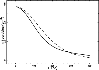
Figure 1: Profiles of density versus scale height $\rm z$: the self-gravitating disk as given by Eq. (5) when $\rm h=90$ pc (dashed) and the three-component exponential distribution as given by Eq. (4) (full line).

Assuming that the expansion starts at $\rm z=0$, we can write $\rm z=R\sin(\theta)$, and therefore

$$n(R,\theta)=n_{0}sech^{2}(\frac{R\sin(\theta)}{2\,h})\quad,$$ (6)

where $\rm R$ is the radius of the advancing shell.

The 3D expansion that starts at the origin of the coordinates will be characterized by the following properties.

• The dependence of the momentary radius of the shell on the latitude angle $\rm\theta$ over the range $\rm[-90^{\circ}\leftrightarrow+90^{\circ}]$.

• The independence of the momentary radius of the shell from $\rm\phi$, the azimuthal angle in the $\rm x$-$\rm y$ plane, which has a range $\rm[0^{\circ}\leftrightarrow 360^{\circ}]$.

The mass swept, $\rm M$, along the solid angle $\rm\Delta\;\Omega$ between 0 and $\rm R$ is

$$M(R,\theta)=\frac{\Delta\;\Omega}{3}m_{H}n_{0}I_{m}(R)+\frac{4}{3}\pi R_{0}^{3}n_{0}m_{H}\quad,$$ (7)

where

$$I_{m}(R)=\int_{R_{0}}^{R}r^{2}sech^{2}(\frac{r\sin(\theta)}{2\,h})dr\quad,$$ (8)

where $\rm R_{0}$ is the initial radius and $\rm m_{H}$ the mass of hydrogen. The integral is

$$\rm\displaystyle I_{m}(R)=-4\,h{r}^{2}(\sin(\theta))^{-1}(1+{{\rm e}^{{\frac{r\sin(\theta)}{h}}}})^{-1}+4\,{\frac{h{r}^{2}}{\sin(\theta)}}$$

$$\rm\displaystyle-8\,{h}^{2}r\ln(1+{{\rm e}^{{\frac{r\sin(\theta)}{h}}}})(\sin(\theta))^{-2}-8\,{h}^{3}{\it\mathrm{Li}_{2}\/}(-{{\rm e}^{{\frac{r\sin(\theta)}{h}}}})(\sin(\theta))^{-3}\quad,$$ (9)

where

$$\mathop{\mathrm{Li}_{2}\/}\nolimits\!\left(z\right)=\sum_{{n=1}}^{\infty}\frac{z^{n}}{n^{2}}\quad,$$ (10)

is the dilogarithm, see Hill (1828); Lewin (1981); Olver et al. (2010).

The conservation of momentum along the solid angle $\rm\Delta\;\Omega$ gives

$$M(R,\theta)\dot{R}(\theta)=M(R_{0})\dot{R_{0}}\quad,$$ (11)

where $\rm\dot{R}(\theta)$ is the velocity at $\rm R$ and $\rm\dot{R_{0}}$ is the initial velocity at $\rm R=R_{0}$. Using the previous equation, an analytical expression for $\rm\dot{R}(\theta)$ along the solid angle can be found, but it is complicated, and therefore we omit it. In this differential equation of the first order in $\rm R$, the variables can be separated and integrating term by term gives

$$\int_{R_{0}}^{R}M(r,\theta)dr=M(R_{0})\dot{R_{0}}\,(t-t_{0})\quad,$$ (12)

where $\rm t$ is the time and $\rm t_{0}$ the time at $\rm R_{0}$. We therefore have an equation of the type

$${\mathcal{F}}(R,R_{0},h)_{NL}=\frac{1}{3}R_{0}^{3}\dot{R_{0}}\,\left(t-{\it t_{0}}\right)\quad,$$ (13)

where $\rm{\mathcal{F}}(R,R_{0},h)_{NL}$ has an analytical but complicated form. The case of expansion that starts from a given galactic height $\rm z$, denoted by $\rm z_{\mathrm{OB}}$, which represent the OB associations, cannot be solved by Eq. (13), which is derived for a symmetrical expansion that starts at $\rm z=0$. It is not possible to find $\rm R$ analytically and a numerical method should be implemented. In our case, in order to find the root of the nonlinear Eq. (13), the FORTRAN subroutine ZRIDDR from Press et al. (1992) has been used.

The following two recursive equations are found when momentum conservation is applied:

$$\rm\displaystyle R_{n+1}=R_{n}+V_{n}\Delta t$$

$$\rm\displaystyle V_{n+1}=V_{n}\Bigl{(}\frac{M_{n}(r_{n})}{M_{n+1}(R_{n+1})}\Bigr{)}\quad,$$ (14)

where $\rm R_{n}$, $\rm V_{n}$, $\rm M_{n}$ are the temporary radius, the velocity, and the total mass, respectively, $\rm\Delta t$ is the time step, and $\rm n$ is the index. The advancing expansion is computed in a 3D Cartesian coordinate system ($\rm x,y,z$) with the centre of the explosion at (0,0,0). The explosion is better visualized in a 3D Cartesian coordinate system ($\rm X,Y,Z$) in which the galactic plane is given by $\rm Z=0$. The following translation, $\rm T_{\mathrm{OB}}$, relates the two Cartesian coordinate systems.

$$T_{\mathrm{OB}}~{}\left\{\begin{array}[]{l}X=x\\ \vskip 6.0pt plus 2.0pt minus 2.0pt\cr Y=y\\ \vskip 6.0pt plus 2.0pt minus 2.0pt\cr Z=z+z_{\mathrm{OB}}\end{array}\right.\quad,$$ (15)

where $\rm z_{\mathrm{OB}}$ is the distance in parsecs of the OB associations from the galactic plane.

The physical units have not yet been specified: parsecs for length and $\rm 10^{7}\,yr$ for time are perhaps an acceptable astrophysical choice. With these units, the initial velocity $\rm V_{{0}}=\dot{R_{0}}$ is expressed in units of pc/($\rm 10^{7}$ yr) and should be converted into km/s; this means that $\rm V_{{0}}=10.207V_{{1}}$ where $\rm V_{{1}}$ is the initial velocity expressed in km/s.

Analytical results can also be obtained solving the Kompaneets equation, see Kompaneets (1960), for the motion of a shock wave in different plane-parallel stratified media such as exponential, power-law type, and a quadratic hyperbolic-secant, see synoptic Table 4 in Olano (2009).

4 Astrophysical applications

A useful formula that allows setting up the initial conditions is formula (10.38) in McCray (1987) which models the SB evolution in the energy conserving phase when the number density is constant,

$$R=111.56\;\mathrm{pc}(\frac{E_{51}t_{7}^{3}N^{*}}{n_{0}})^{\frac{1}{5}},$$ (16)

where $\rm t_{7}$ is the time expressed in units of $\rm 10^{7}$ yr, $\rm E_{51}$ is the energy expressed in units of $\rm 10^{51}$ erg, $\rm n_{0}$ is the number density expressed in particles $\rm\mathrm{cm}^{-3}$ (density $\rm\rho_{0}=n_{0}m$, where $\rm m=1.4m_{\mathrm{H}}$) and $\rm N^{*}$ is the number of SN explosions in $\rm 5.0\cdot 10^{7}$ yr and therefore is a rate, see McCray (1987). This formula, deduced in spherical coordinates, can be used only when the density is constant, as an example for the first 20 pc, the variation of the density with galactic height is $\rm\approx~{}2\%$. In the following, we will assume that the bursting phase ends at $\rm t=t_{7,0}$ (the bursting time is expressed in units of $\rm 10^{7}$ yr) when $\rm N_{SN}$ SN are exploded

$$N_{SN}=N^{*}\frac{t_{7,0}\cdot 10^{7}}{5\cdot 10^{7}}\quad.$$ (17)

The velocity of the SB in the energy conserving phase when the number density is constant is

$$V(t_{7})=\frac{6.567\,\sqrt[5]{{\frac{{\it E51}\,{\it N^{*}}}{{\it n_{0}}}}}}{{{\it t_{7}}}^{2/5}}\frac{km}{s}\quad.$$ (18)

Eq. (16) and (18) can be used to deduce $\rm R_{0}$ and and $\rm V_{0}$ once $\rm N^{*}$ and $\rm t_{7,0}$ are given. We continue giving some information about the astrophysical target of our simulation, analysing the analytical solution at $\rm z_{\mathrm{OB}}$ =0 and the numerical solution $\rm z_{\mathrm{OB}}\neq 0$, making a comparison with the hydro code and analysing the effects of the galactic rotation on the obtained results.

4.1 The simulated object

When the two worms 46.4+5.5 and 39.7+5.7 are carefully studied (Kim & Koo (2000)) it is possible to conclude that they belong to a single SB. The parameters of this single SB are given in Table 1.

Table 1: Data of the SB associated with GW 46.4+5.5.

$$\rm\rm\begin{array}[]{cc}\hline\cr\vskip 3.0pt plus 1.0pt minus 1.0pt\cr\mbox{Dimensions~{}(pc}^{2})&345\times 540\\ \mbox{Expansion~{}velocity~{} (km~{}s$\rm{}^{-1}$})&15\\ \mbox{Age~{}(10$\rm{}^{7}$~{}yr})&0.5\\ \mbox{z$\rm{}_{OB}$ (pc)}&100\\ \mbox{Total~{}energy~{}($\rm 10^{51}$}{\mathrm{erg}})&15\\ \vskip 3.0pt plus 1.0pt minus 1.0pt\cr\hline\cr\end{array}$$

4.2 Analytical versus numerical solutions

The analytical model as given by the solution of the nonlinear Eq. (13) can be used only in the case $\rm z_{\mathrm{OB}}$=0. As an example, we give a model of the SB associated with GW 46.4+5.5, see Fig. 2.

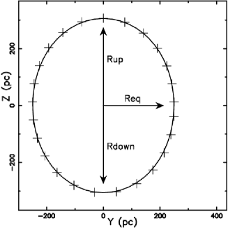
Figure 2: Section of the SB GW 46.4+5 in the Y-Z;X=0 plane when the explosion starts at $\rm z_{\mathrm{OB}}=0\mbox{pc}$. The analytical results are shown as full line and the numerical results as crosses. The code parameters of the solution of Eq. (13) as well of the numerical couple (14) are $\rm h=90$ pc, $\rm t_{7}=0.45~{}$, $\rm t_{7,0}$ = 0.0045, $\rm r_{0}$ = 49.12, $\rm V_{0}=641.7\,\mathrm{km}\,\mathrm{s}^{-1}$, $\rm N_{SN}$ = 93 and $\rm N^{*}$=103000.

The numerical solution as given by the recursive relationship (14) can be found adopting the same input data of the analytical solution, see crosses in Fig. (2); the numerical solution agrees with the analytical solution within 0.65%. We are now ready to present the numerical evolution of the SB associated with GW 46.4+5 when $\rm z_{\mathrm{OB}}=100\mbox{pc}$, see Fig. 3 and Table 2.

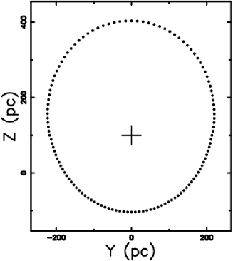
Figure 3: Section of the SB GW 46.4+5 in the Y-Z;X=0 plane when the explosion starts at $\rm z_{\mathrm{OB}}=100\mbox{pc}$. The code parameters for the numerical couple (14) are $\rm h=90$ $\rm pc$, $\rm t_{7}=0.45~{}$, $\rm t_{7,0}$ = 0.00045, $\rm r_{0}$ = 24.43, $\rm V_{0}=3191\mathrm{km}\,\mathrm{s}^{-1}$, $\rm N_{SN}$ = 180 and $\rm N^{*}$=2000000. The explosion site is represented by a cross.

Table 2: Simulated data of the SB associated with GW 46.4+5.5.

$$\rm\rm\begin{array}[]{cc}\hline\cr\vskip 3.0pt plus 1.0pt minus 1.0pt\cr\mbox{Size~{}(pc}^{2})&454\cdot 521\\ \mbox{Averaged expansion~{}velocity~{} (km~{}s$\rm{}^{-1}$})&19.3\\ \mbox{Age~{}(10$\rm{}^{7}$~{}yr})&0.45\\ \mbox{z$\rm{}_{OB}$ (pc)}&100\\ \vskip 3.0pt plus 1.0pt minus 1.0pt\cr\hline\cr\end{array}$$

4.3 Numerical solution and hydro code

The level of confidence in our results can be given by a comparison with numerical hydro-dynamics calculations (see, for example, Mac Low et al. (1989)). The vertical density distribution they adopted, see equation (1) in Mac Low et al. (1989) and equation (5) in Tomisaka & Ikeuchi (1986), has the following dependence on $\rm z$, the distance from the galactic plane in parsec:

$$n_{\mathrm{hydro}}=n_{\mathrm{d}}\left\{\Theta{\mathrm{exp}}[-\frac{V_{p}(z)}{\sigma_{{\mathrm{IC}}}^{2}}]+(1-\Theta){\mathrm{exp}}\left[-\frac{V_{p}(z)}{\sigma_{{\mathrm{{\mathrm{C}}}}}^{2}}\right]\right\},$$ (19)

with the gravitational potential

$$V_{p}(z)=68.6{\mathrm{ln}}\left[1+0.9565~{}{\mathrm{sinh}}^{2}\left(0.758\frac{z}{z_{0}}\right)\right]({\mathrm{kms}}^{-1})^{2}.$$ (20)

Here, $\rm n{\mathrm{{}_{d}}}=1~{}\mbox{particles~{}cm}^{-3}$, $\rm\Theta=0.22$, $\rm\sigma_{IC}=14.4{\mathrm{km~{}s}}^{-1}$, $\rm\sigma_{C}=7.1{\mathrm{km~{}s}}^{-1}$, and $\rm z_{0}=124~{}{\mathrm{pc}}$. Fig. (4) compares the hydro number density as given by Eq. 19 and the theoretical function as given by Eq. (5). The difference in the density profiles from hydrosimulations and from the simple model adopted in this paper are due to the fact that the density at $\rm z=0$ is assumed to be $\rm n_{\mathrm{hydro}}=1~{}\mbox{particles~{}cm}^{-3}$ in the hydrosimulations, see Mac Low et al. (1989). In our model conversely at $\rm z=0$ we have $\rm n=0.566~{}\mbox{particles~{}cm}^{-3}$ as in Lockman (1984).

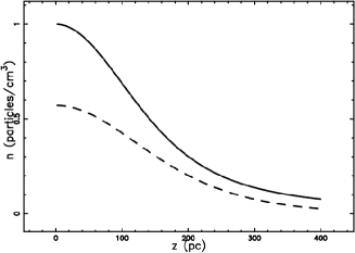
Figure 4: Profiles of density versus scale height $\rm z$: the self-gravitating disk as in Eq. (5) when $\rm h=90$ pc (dashed line) and the hydro number density as given by Eq. 19 (full line).

A typical run of ZEUS (see Mac Low et al. (1989)), a two-dimensional hydrodynamic code, is done for $\rm t_{7}=0.45$ and supernova luminosity of $\rm 1.6\cdot 10^{38}{\mathrm{erg~{}s}}^{-1}$ when $\rm z_{\mathrm{OB}}$=100 pc. In order to make a comparison with our code, we adopt the same time and we search the parameters which produce similar results, see Fig. 5.

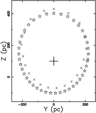
Figure 5: Section of the SB in the X-Z plane when the explosion starts at $\rm z_{\mathrm{OB}}=100\mbox{pc}$ (empty stars). The code parameters are $\rm h=90$ pc, $\rm t_{7}=0.45~{}$, $\rm t_{7,0}$ = 0.00045, $\rm r_{0}$ = 24.43, $\rm V_{0}=3191\,\mathrm{km}\,\mathrm{s}^{-1}$, $\rm N_{SN}$ = 180 and $\rm N^{*}$=2000000. The points represented by the small crosses indicate the inner section from Fig. 3a of MacLow et al. 1989. The explosion site is represented by a big cross.

The percentage of reliability of our code can also be introduced,

$$\epsilon=(1-\frac{|(R_{\mathrm{hydro}}-R_{\mathrm{num}})|}{R_{\mathrm{hydro}}})\cdot 100\,,$$ (21)

where $\rm R_{\mathrm{hydro}}$ is the radius given by the hydro-dynamics, and $\rm R_{\mathrm{num}}$ s the radius obtained from our simulation. Table 3 shows our numerical radii in the upward, downward, and equatorial directions, and the efficiency as given by formula (21).

Table 3: Code reliability.

$$\rm\rm\begin{array}[]{ccccc}\hline\cr\vskip 3.0pt plus 1.0pt minus 1.0pt\cr{}{}{}{}\hfil&R_{\mathrm{up}}(\mathrm{pc})&R_{\mathrm{down}}(\mathrm{pc})&R_{\mathrm{eq}}(\mathrm{pc})\\ \vskip 3.0pt plus 1.0pt minus 1.0pt\cr\hline\cr\vskip 3.0pt plus 1.0pt minus 1.0pt\cr R_{\mathrm{hydro}}(ZEUS)&330&176&198\\ R_{\mathrm{num}}(\mbox{our~{}code})&302&203&217\\ \mbox{efficiency}(\%)&91&84&90\\ \vskip 3.0pt plus 1.0pt minus 1.0pt\cr\hline\cr\end{array}$$

4.4 Galactic rotation

The influence of the Galactic rotation on the results can be be obtained by introducing the law of the Galactic rotation as given by Wouterloot et al. (1990),

$$V_{\mathrm{R}}(R_{0})=220(\frac{R_{0}[\mathrm{pc}]}{8500})^{0.382}\mathrm{km~{}sec}^{-1},$$ (22)

where $\rm R_{0}$ is the radial distance from the centre of the Galaxy in parsecs. The original circular shape of the superbubble at a given value of $\rm z$ transforms to an ellipse by the following transformation, $\rm T_{\mathrm{r}}$,

$$T_{\mathrm{r}}~{}\left\{\begin{array}[]{l}x\prime=x+0.264y~{}t\\ \vskip 6.0pt plus 2.0pt minus 2.0pt\cr y\prime=y\\ \vskip 6.0pt plus 2.0pt minus 2.0pt\cr z\prime=z,\end{array}\right.$$ (23)

where y is in parsecs and $\rm t$ is expressed in units of $\rm 10^{7}~{}{\mathrm{yr}}$ Zaninetti (2004), see Fig. 6.

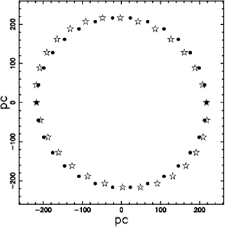
Figure 6: Section of the SB GW 46.4+5 in the Y-X,Z=0 plane when the explosion starts at $\rm z_{\mathrm{OB}}=100\mbox{pc}$. Full points represent the circular section, the empty stars the rotation-distorted section. Parameters as in Fig. 3 and $\rm R_{0}[\mathrm{pc}]$=8500.

In the same way, the effect of the shear velocity as a function of the distance $\rm y$ from the centre of the expansion, $\rm V_{shift}(y)$, can be easily obtained by performing a Taylor expansion of Eq. (22)

$$V_{shift}(y)=84.04\frac{y}{R_{0}}\,Km/s\quad.$$ (24)

This is the the shear velocity as a function of $\rm y$. Fig. 7 shows the rotation-distorted map of position and velocity.

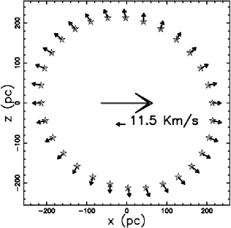
Figure 7: The stars represent the rotation-distorted section when $\rm R_{0}[\mathrm{pc}]$=8500. The arrows show the velocity field of the expansion as modified by the shear velocity. The direction of rotation of the Galaxy (big arrow) and the scale of the velocity are shown.

The effect of rotation seems to be small and in order to see a more relevant correction we should increase the elapsed time, see Fig. 8.

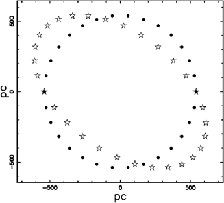
Figure 8: Section of the SB GW 46.4+5 in the Y-X,Z=0 plane when the explosion starts at $\rm z_{\mathrm{OB}}=100\mbox{pc}$. Full points represent the circular section and the empty stars the rotation-distorted section. Parameters as in Fig. 3 except $\rm t_{7}=2~{}$ and $\rm R_{0}[\mathrm{pc}]$=8500.

5 The image

The transfer equation in the presence of emission only, see for example Rybicki & Lightman (1991) or Hjellming, R. M. (1988), is

$$\frac{dI_{\nu}}{ds}=-k_{\nu}\zeta I_{\nu}+j_{\nu}\zeta\quad,$$ (25)

where $\rm I_{\nu}$ is the specific intensity, $\rm s$ is the line of sight, $\rm j_{\nu}$ the emission coefficient, $\rm k_{\nu}$ a mass absorption coefficient, $\rm\zeta$ the mass density at position $\rm s$, and the index $\rm\nu$ denotes the relevant frequency of emission. The solution to Eq. (25) is

$$I_{\nu}(\tau_{\nu})=\frac{j_{\nu}}{k_{\nu}}(1-e^{-\tau_{\nu}(s)})\quad,$$ (26)

where $\rm\tau_{\nu}$ is the optical depth at frequency $\rm\nu$

$$d\tau_{\nu}=k_{\nu}\zeta ds\quad.$$ (27)

We now continue analysing the case of an optically thin layer in which $\rm\tau_{\nu}$ is very small ( or $\rm k_{\nu}$ very small ) and the density $\rm\zeta$ is replaced with our number density $\rm C(s)$ of particles. One case is taken into account: the emissivity is proportional to the number density

$$j_{\nu}\zeta=KC(s)\quad,$$ (28)

where $\rm K$ is a constant. This can be the case for synchrotron emission and a simple model for the acceleration of the electrons can be found in Appendix A. We select as an example the [S II] continuum of the synchrotron superbubble in the irregular galaxy IC10, see Lozinskaya et al. (2008), and the X-ray emission below 2 keV around the OB association LH9 in the H II complex N11 in the Large Magellanic Cloud, see Maddox et al. (2009). The intensity at a given frequency is

$$I(\nu)\propto l\nu^{\beta}\quad,$$ (29)

where $\rm l$ is the length of the radiating region along the line of sight. The source of synchrotron luminosity is assumed here to be the rate of kinetic energy, $\rm L_{m}$,

$$L_{m}=\frac{1}{2}\rho AV^{3}\quad,$$ (30)

where $\rm A$ is the considered area, see formula (A28) in De Young (2002). In the case of formula (16) $\rm A=4\pi R^{2}$, which means

$$L_{m}=\frac{1}{2}\rho 4\pi R^{2}V^{3}\quad,$$ (31)

where $\rm R$ is the instantaneous radius of the SB and $\rm\rho$ is the density in the advancing layer in which the synchrotron emission takes place. The astrophysical version of the the rate of kinetic energy,

$$L_{ma}={1.39\times 10^{29}}\,{\it n_{1}}\,{{\it R_{1}}}^{2}{{\it V_{1}}}^{3}\frac{ergs}{s}\quad,$$ (32)

where $\rm n_{1}$ is the number density expressed in units of $\rm 1~{}\frac{particle}{cm^{3}}$, $\rm R_{1}$ is the radius in parsecs, and $\rm V_{1}$ is the velocity in km/s. The spectral luminosity, $\rm L_{\nu}$, at a given frequency $\rm\nu$ is

$$L_{\nu}=4\pi D^{2}S_{\nu}\quad,$$ (33)

with

$$S_{\nu}=S_{0}(\frac{\nu}{\nu_{0}})^{\beta}\quad,$$ (34)

where $\rm S_{0}$ is the flux observed at the frequency $\rm\nu_{0}$ and $\rm D$ is the distance. The total observed synchrotron luminosity, $\rm L_{tot}$, is

$$L_{tot}=\int_{\nu_{min}}^{\nu_{max}}L_{\nu}d\nu\quad,$$ (35)

where $\rm{\nu_{min}}$ and $\rm{\nu_{max}}$ are the minimum and maximum frequencies observed. The total observed luminosity can be expressed as

$$L_{tot}=\epsilon L_{ma}\quad,$$ (36)

where $\rm\epsilon$ is a constant of conversion from the mechanical luminosity to the total observed luminosity in synchrotron emission.

The fraction of the total luminosity deposited in a band $\rm f_{c}$ is

$$f_{c}=\frac{{{\it\nu_{c,min}}}^{\beta+1}-{{\it\nu_{c,max}}}^{\beta+1}}{{{\it\nu_{min}}}^{\beta+1}-{{\it\nu_{max}}}^{\beta+1}}\quad,$$ (37)

where $\rm\nu_{c,min}$ and $\rm\nu_{c,max}$ are the minimum and maximum frequency of the band. Table 4 shows some values of $\rm f_{c}$ for the most important optical bands.

Table 4: Table of the values of $\rm f_{c}$ when $\rm\nu_{min}=10^{7}Hz$, $\rm\nu_{max}=10^{18}Hz$ and $\rm\beta=-0.7$.

band	$\rm\lambda$ ($\rm\AA$)	FWHM ($\rm\AA$)	$\rm f_{c}$
U	3650	700	6.86 $\rm\times 10^{-3}$
B	4400	1000	7.70 $\rm\times 10^{-3}$
V	5500	900	5.17 $\rm\times 10^{-3}$
$\rm H\alpha$	6563	100	0.56 $\rm\times 10^{-3}$
$\rm[SII]$ continuum	7040	210	0.92 $\rm\times 10^{-3}$

An analytical solution for the radial cut of intensity of emission can be found in the equatorial plane $\rm z_{\mathrm{OB}}$=0. We assume that the number density of relativistic electrons $\rm C$ is constant and in particular rises from 0 at $\rm r=a$ to a maximum value $\rm C_{m}$, remains constant up to $\rm r=b$, and then falls again to 0, see Zaninetti (2009). This geometrical description is shown in Fig. 9.

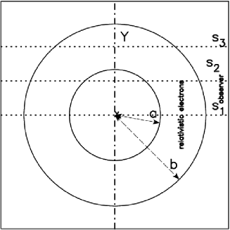
Figure 9: The two circles (sections of spheres) which include the region with constant density are represented through a full line. The observer is situated along the $\rm x$ direction, three lines of sight are indicated, and the relativistic electrons have radius $\rm r$ in the region $\rm a<r<b$.

The length of sight, when the observer is situated at the infinity of the $\rm x$-axis, is the locus parallel to the $\rm x$-axis which crosses the position $\rm y$ in a Cartesian $\rm x-y$ plane and terminates at the external circle of radius $\rm b$. When the number density of the relativistic electrons $\rm C_{m}$ is constant between the two spheres of radii $\rm a$ and $\rm b$, the intensity of radiation is

$$\rm\displaystyle I_{0a}=C_{m}\times 2\times(\sqrt{b^{2}-y^{2}}-\sqrt{a^{2}-y^{2}})\quad;0\leq y<a$$

$$\rm\displaystyle I_{ab}=C_{m}\times 2\times(\sqrt{b^{2}-y^{2}})\quad;a\leq y<b\quad.$$ (38)

The ratio between the theoretical intensity at the maximum ($\rm(y=a)$) and at the minimum ($\rm y=0$) is given by

$$\frac{I(y=a)}{I(y=0)}=\frac{\sqrt{b^{2}-a^{2}}}{b-a}\quad.$$ (39)

A cut in the theoretical intensity of the SB associated with GW 46.4+5.5 is shown in Fig. 10.

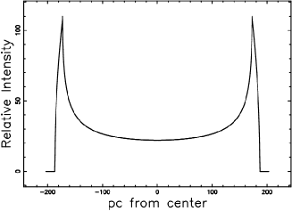
Figure 10: Cut of the mathematical intensity $\rm{\it I}$ of the ring model, Eq. (38), in the equatorial plane (full line) of the SB associated with GW 46.4+5.5 . The $\rm x$- and $\rm y$-axes are in pc, $\rm a=172.5$ pc, $\rm b=186.9$ pc and $\rm\frac{I(y=a)}{I(y=0)}=5$.

Similar analytical results for the intensity of the cuts in the H$\rm\alpha$ of planetary nebulae and in the radio of supernova remnants have been found by Gray et al. (2012), compare their Figure 5 with our Figure 9 and by Opsenica & Arbutina (2011), see their Figure 1. A simulated image of the complex shape of a SB is composed by combining the intensities which characterize different points of the advancing shell. For an optically thin medium, the transfer equation provides the emissivity to be multiplied with the distance on the line of sight, $\rm l$. This length in SB depends on the orientation of the observer but for the sake of clarity the observer is at infinity and sees the SB from the equatorial plane $\rm z_{\mathrm{OB}}$ =0 or from one of the two poles. We now outline the numerical algorithm which allows us to build the complex image of an SB.

• An empty (value=0) memory grid $\rm{\mathcal{M}}(i,j,k)$ which contains $\rm NDIM^{3}$ pixels is considered

• We first generate an internal 3D surface by rotating the section of $\rm 180^{\circ}$ around the polar direction and a second external surface at a fixed distance $\rm\Delta R$ from the first surface. As an example, we fixed $\rm\Delta R$ = $\rm 0.03R_{max}$, where $\rm R_{max}$ is the maximum radius of expansion. The points on the memory grid which lie between the internal and the external surfaces are memorized on $\rm{\mathcal{M}}(i,j,k)$ with a variable integer number according to formula (31) and density $\rm\rho$ proportional to the swept mass.

• Each point of $\rm{\mathcal{M}}(i,j,k)$ has spatial coordinates $\rm x,y,z$ which can be represented by the following $\rm 1\times 3$ matrix, $\rm A$,

  $$A=\left[\begin{array}[]{c}x\\ \vskip 6.0pt plus 2.0pt minus 2.0pt\cr y\\ \vskip 6.0pt plus 2.0pt minus 2.0pt\cr{\it z}\end{array}\right]\quad.$$ (40)

  The orientation of the object is characterized by the Euler angles $\rm(\Phi,\Theta,\Psi)$ and therefore by a total $\rm 3\times 3$ rotation matrix, $\rm E$, see Goldstein et al. (2002). The matrix point is represented by the following $\rm 1\times 3$ matrix, $\rm B$,

  $$B=E\cdot A\quad.$$ (41)

• The intensity map is obtained by summing the points of the rotated images along a particular direction.

• The effect of the insertion of a threshold intensity, $\rm I_{tr}$, given by the observational techniques, is now analysed. The threshold intensity can be parametrized by $\rm I_{max}$, the maximum value of intensity which characterizes the map, see Zaninetti (2012).

An ideal image of the intensity of SB GW 46.4+5 is shown in Fig. 11, and Fig. 12 shows two cuts through the centre of the SB.

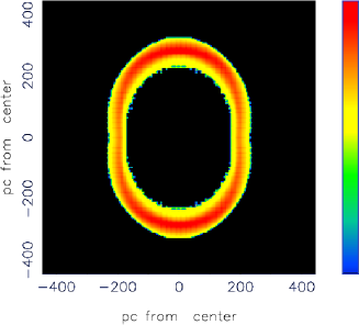
Figure 11: Map of the theoretical intensity of SB GW 46.4+5. Physical parameters as in Fig. 2. The three Euler angles characterizing the orientation are $\rm\Phi$=90 ^∘, $\rm\Theta$=90 ^∘ and $\rm\Psi$=90 ^∘. This combination of Euler angles corresponds to the rotated image with the polar axis along the z-axis. In this map $\rm I_{tr}=I_{max}/2.$

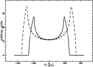
Figure 12: Two cuts of the model intensity across the centre of the SB: equatorial cut (full line) and polar cut (dotted line). Parameters as in Fig.  11 and $\rm I_{tr}=0$.

We can also build the theoretical image as seen from one of the two poles, see Fig. 13.

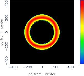
Figure 13: Map of the theoretical intensity of SB GW 46.4+5 as seen from the polar direction at infinity. Physical parameters as in Fig. 2. The three Euler angles characterizing the orientation are $\rm\Phi$=0^∘, $\rm\Theta$=0^∘ and $\rm\Psi$=0^∘. In this map $\rm I_{tr}=I_{max}/2.$

6 Conclusions

Law of motion The temporal evolution of an SB in a medium with constant density is characterized by a spherical symmetry. The presence of a thin self-gravitating disk of gas which is characterized by a Maxwellian distribution in velocity and distribution of density which varies only in the z-direction produces an axial symmetry in the temporal evolution of an SB. The resulting Eq. (13) has an analytical form which can be solved numerically when $\rm z_{\mathrm{OB}}$ =0. The case of $\rm z_{\mathrm{OB}}\neq 0$ can be attached solving two recursive equations, see (14). These complex shapes can also be modeled by the Kompaneets equation when a quadratic hyperbolic-secant is adopted. Both the approximation here used and the Kompaneets equation can model the shape of the SB without invoking the collision of two wind-blown SBs, see Ntormousi et al. (2011). The code developed here runs in less than a minute on a LINUX -$\rm 2.66$GHz processor and can be an alternative to a purely numerical 2D or 3D model.

Synchrotron Emission

Here we assumed that the conversion from the flux of kinetic energy into non thermal luminosity is regulated by a constant. The exact value of this constant can be deduced once the number density, radius, thickness, and velocity of the advancing shell are provided by observational astronomy. The values of the fraction of flux deposited in the various astronomical bands, $\rm f_{c}$, are given in Table 4.

Images

The emissivity in the thin advancing layer is assumed to be proportional to the rate of kinetic energy, see Eq. (30), where the density is assumed to be proportional to the swept material. This assumption explains the strong limb-brightening visible on the astronomical maps of SBs and allows associating the observed worms to the non detectable SBs. As an example, if the threshold of the observable flux at a given wavelength is bigger than the emitted flux at the centre of an SB, we will detect only the external regions, the so called worms, see Fig. 12.

Appendix A How to accelerate electrons

An electron which loses its energy due to synchrotron radiation has a lifetime of

$$\tau_{r}\approx\frac{E}{P_{r}}\approx 500E^{-1}H^{-2}sec\quad,$$ (42)

where $\rm E$ is the energy in ergs, $\rm H$ the magnetic field in Gauss, and $\rm P_{r}$ is the total radiated power (Lang, 1999, Eq. 1.157). The energy is connected to the critical frequency (Lang, 1999, Eq. 1.154), by

$$\nu_{c}=6.266\times 10^{18}HE^{2}~{}\mathrm{Hz}\quad.$$ (43)

The lifetime for synchrotron losses is

$$\tau_{syn}=39660\,{\frac{1}{H\sqrt{H\nu}}}\,\mathrm{yr}\quad.$$ (44)

Following (Fermi, 1949, 1954), the gain in energy in a continuous form for a particle which spirals around a line of force is proportional to its energy, $\rm E$,

$$\frac{dE}{dt}=\frac{E}{\tau_{II}}\quad,$$ (45)

where $\rm\tau_{II}$ is the typical time-scale,

$$\frac{1}{\tau_{II}}=\frac{4}{3}(\frac{u^{2}}{c^{2}})(\frac{c}{L_{II}})\quad,$$ (46)

where $\rm u$ is the velocity of the accelerating cloud belonging the advancing shell of the SB, $\rm c$ is the velocity of light, and $\rm L_{II}$ is the mean free path between clouds (Lang, 1999, Eq. 4.439). The mean free path between the accelerating clouds in the Fermi II mechanism can be found from the following inequality in time:

$$\tau_{II}<\tau_{sync}\quad,$$ (47)

which corresponds to the following inequality for the mean free path between scatterers

$$L<\frac{1.72\,10^{5}\,{u}^{2}}{H\sqrt{H\nu}{c}^{2}}\,\mathrm{pc}\quad.$$ (48)

The mean free path length for an SB at [S II] continuum, which means 7040 $\rm\AA$ or 704 nm or $\rm 4.258\,10^{14}$ Hz, gives

$$L<\frac{2.94\,10^{-6}\,{{\it u_{1}}}^{2}}{{{\it H_{5}}}^{3/2}}\,\mathrm{pc}$$ (49)

where $\rm u_{1}$ is the velocity of the accelerating cloud expressed in km/s, and $\rm H_{5}=$ is the magnetic field expressed in units of $\rm 10^{-5}$ Gauss. When this inequality is verified, the direct conversion of the rate of kinetic energy into radiation can be adopted. Recall that the Fermi II mechanism produces an inverse power law spectrum in the energy of the type $\rm N(E)\propto E^{-\gamma}$ or an inverse power law in the observed frequencies $\rm N(\nu)\propto\nu^{\beta}$ with $\rm\beta=-\frac{\gamma-1}{2}$ (Lang, 1999; Zaninetti, 2011). The strong shock accelerating mechanism named Fermi I was introduced by Bell (1978a) and Bell (1978b). The energy gain relative to a particle that is crossing the shock is:

$$\frac{dE}{dt}=\frac{E}{\tau_{I}}\quad,$$ (50)

where $\rm\tau_{I}$ is the typical time-scale,

$$\frac{1}{\tau_{I}}=\frac{2}{3}(\frac{u}{c})(\frac{c}{L_{I}})\quad,$$ (51)

where $\rm u$ is the velocity of the shock of the SB, $\rm c$ is the velocity of light, and $\rm L_{I}$ is the mean free path between scatterers. This process produces an energy spectrum of electrons of the type:

$$N(E)dE\propto E^{-2}dE\quad,$$ (52)

see Longair (1994). The two mechanisms , Fermi I and Fermi II, produce the same results when

$$\frac{L_{II}}{L_{I}}=2\frac{u}{c}\quad.$$ (53)

References

- Baek et al. (2008) Baek C. H., Kudoh T., Tomisaka K., 2008, ApJ , 682, 434
- Bell (1978a) Bell A. R., 1978a, MNRAS , 182, 147
- Bell (1978b) Bell A. R., 1978b, MNRAS , 182, 443
- Bertin (2000) Bertin G., 2000, Dynamics of Galaxies. Cambridge University Press., Cambridge
- Bisnovatyi-Kogan & Silich (1995) Bisnovatyi-Kogan G. S., Silich S. A., 1995, Rev. Mod. Phys. , 67, 661
- Butt & Bykov (2008) Butt Y. M., Bykov A. M., 2008, ApJ , 677, L21
- Chu (2008) Chu Y.-H., 2008, in F. Bresolin, P. A. Crowther, & J. Puls ed., IAU Symposium Vol. 250 of IAU Symposium, Bubbles and Superbubbles: Observations and Theory. pp 341–354
- De Young (2002) De Young D. S., 2002, The physics of extragalactic radio sources. University of Chicago Press, Chicago
- Dickey & Lockman (1990) Dickey J. M., Lockman F. J., 1990, ARA&A , 28, 215
- Dyson, J. E. and Williams, D. A. (1997) Dyson, J. E. and Williams, D. A. 1997, The physics of the interstellar medium. Institute of Physics Publishing, Bristol
- English et al. (2000) English J., Taylor A. R., Mashchenko S. Y., Irwin J. A., Basu S., Johnstone D., 2000, ApJ , 533, L25
- Fermi (1949) Fermi E., 1949, Physical Review, 75, 1169
- Fermi (1954) Fermi E., 1954, ApJ , 119, 1
- Ferrand & Marcowith (2010) Ferrand G., Marcowith A., 2010, A&A , 510, A101
- Goldstein et al. (2002) Goldstein H., Poole C., Safko J., 2002, Classical mechanics. Addison-Wesley, San Francisco
- Gray et al. (2012) Gray M. D., Matsuura M., Zijlstra A. A., 2012, MNRAS , 422, 955
- Higdon & Lingenfelter (2005) Higdon J. C., Lingenfelter R. E., 2005, ApJ , 628, 738
- Higdon & Lingenfelter (2006) Higdon J. C., Lingenfelter R. E., 2006, Advances in Space Research, 37, 1913
- Hill (1828) Hill C. J., 1828, J. Reine Angew. Math., 3, 101
- Hjellming, R. M. (1988) Hjellming, R. M. 1988, Radio stars IN Galactic and Extragalactic Radio Astronomy . Springer-Verlag, New York
- Jaskot et al. (2011) Jaskot A. E., Strickland D. K., Oey M. S., Chu Y.-H., García-Segura G., 2011, ApJ , 729, 28
- Kim & Koo (2000) Kim K.-T., Koo B.-C., 2000, ApJ , 529, 229
- Kompaneets (1960) Kompaneets A. S., 1960, Soviet Phys. Dokl., 5, 46
- Koo et al. (1992) Koo B.-C., Heiles C., Reach W. T., 1992, ApJ , 390, 108
- Lang (1999) Lang K. R., 1999, Astrophysical formulae. (Third Edition). Springer, New York
- Lewin (1981) Lewin L., 1981, Polylogarithms and associated functions.. North Holland, New York
- Lockman (1984) Lockman F. J., 1984, ApJ , 283, 90
- Longair (1994) Longair M. S., 1994, High energy astrophysics. Cambridge University Press, 2nd ed., Cambridge
- Lozinskaya et al. (2008) Lozinskaya T. A., Moiseev A. V., Podorvanyuk N. Y., Burenkov A. N., 2008, Astronomy Letters, 34, 217
- Mac Low & McCray (1988) Mac Low M.-M., McCray R., 1988, ApJ , 324, 776
- Mac Low et al. (1989) Mac Low M.-M., McCray R., Norman M. L., 1989, ApJ , 337, 141
- Maddox et al. (2009) Maddox L. A., Williams R. M., Dunne B. C., Chu Y.-H., 2009, ApJ , 699, 911
- McCray & Kafatos (1987) McCray R., Kafatos M., 1987, ApJ , 317, 190
- McCray (1987) McCray R. A., 1987, in A. Dalgarno & D. Layzer ed., Spectroscopy of Astrophysical Plasmas Coronal interstellar gas and supernova remnants. Cambridge University Press, Cambridge, pp 255–278
- Melioli et al. (2009) Melioli C., Brighenti F., D’Ercole A., de Gouveia Dal Pino E. M., 2009, MNRAS , 399, 1089
- Ntormousi et al. (2011) Ntormousi E., Burkert A., Fierlinger K., Heitsch F., 2011, ApJ , 731, 13
- Oey et al. (2002) Oey M. S., Groves B., Staveley-Smith L., Smith R. C., 2002, AJ , 123, 255
- Olano (2009) Olano C. A., 2009, A&A , 506, 1215
- Olver et al. (2010) Olver F. W. J. e., Lozier D. W. e., Boisvert R. F. e., Clark C. W. e., 2010, NIST handbook of mathematical functions.. Cambridge University Press. , Cambridge
- Opsenica & Arbutina (2011) Opsenica S., Arbutina B., 2011, Serbian Astronomical Journal, 183, 75
- Padmanabhan (2001) Padmanabhan P., 2001, Theoretical astrophysics. Vol. II: Stars and Stellar Systems. Cambridge University Press, Cambridge, MA
- Padmanabhan (2002) Padmanabhan P., 2002, Theoretical astrophysics. Vol. III: Galaxies and Cosmology. Cambridge University Press, Cambridge, MA
- Press et al. (1992) Press W. H., Teukolsky S. A., Vetterling W. T., Flannery B. P., 1992, Numerical Recipes in FORTRAN. The Art of Scientific Computing. Cambridge University Press, Cambridge
- Rafikov & Kulsrud (2000) Rafikov R. R., Kulsrud R. M., 2000, MNRAS , 314, 839
- Rodríguez-González et al. (2011) Rodríguez-González A., Velázquez P. F., Rosado M., Esquivel A., Reyes-Iturbide J., Toledo-Roy J. C., 2011, ApJ , 733, 34
- Rohlfs (1977) Rohlfs K., ed. 1977, Lectures on density wave theory Vol. 69 of Lecture Notes in Physics, Berlin Springer Verlag
- Rybicki & Lightman (1991) Rybicki G., Lightman A., 1991, Radiative Processes in Astrophysics. Wiley-Interscience, New-York
- Smith (2002) Smith N., 2002, MNRAS , 337, 1252
- Spitzer (1942) Spitzer Jr. L., 1942, ApJ , 95, 329
- Tomisaka (1992) Tomisaka K., 1992, PASJ , 44, 177
- Tomisaka & Ikeuchi (1986) Tomisaka K., Ikeuchi S., 1986, PASJ , 38, 697
- Wouterloot et al. (1990) Wouterloot J. G. A., Brand J., Burton W. B., Kwee K. K., 1990, A&A , 230, 21
- Zaninetti (2004) Zaninetti L., 2004, PASJ , 56, 1067
- Zaninetti (2009) Zaninetti L., 2009, MNRAS , 395, 667
- Zaninetti (2010) Zaninetti L., 2010, Advances in Space Research, 46, 1341
- Zaninetti (2011) Zaninetti L., 2011, Astrophysics and Space Science , 333, 99
- Zaninetti (2012) Zaninetti L., 2012, Astrophysics and Space Science, 337, 581