Off-equilibrium photon production during the chiral phase transition

Abstract

In the early stage of ultrarelativistic heavy-ion collisions chiral symmetry is restored temporarily. During this so-called chiral phase transition, the quark masses change from their constituent to their bare values. This mass shift leads to the spontaneous non-perturbative creation of quark-antiquark pairs, which effectively contributes to the formation of the quark-gluon plasma. We investigate the photon production induced by this creation process. We provide an approach that eliminates possible unphysical contributions from the vacuum polarization and renders the resulting photon spectra integrable in the ultraviolet domain. The off-equilibrium photon numbers are of quadratic order in the perturbative coupling constants while a thermal production is only of quartic order. Quantitatively, we find, however, that for the most physical mass-shift scenarios and for photon momenta larger than 1 GeV the off-equilibrium processes contribute less photons than the thermal processes.

I Introduction

Ultrarelativistic heavy-ion collision experiments allow for studying strongly interacting matter under extreme conditions. Such experiments are currently performed at the Relativistic Heavy Ion Collider (RHIC) at the Brookhaven National Laboratory (BNL) and at the Large Hadron Collider (LHC) at the European Organization for Nuclear Research (CERN). Furthermore, they will be carried out at the future Facility for Antiproton and Ion Research (FAIR) at the Helmholtz Center for Heavy Ion Research (GSI) and at the future Nuclotron-based Ion Collider Facility (NICA) at the Joint Institute for Nuclear Research (JINR). One main objective of these experiments is the creation and exploration of the so-called quark-gluon plasma (QGP), a state of matter of deconfined quarks and gluons. The two basic features of the strong interaction, namely confinement Bali and Schilling (1992) and asymptotic freedom Gross and Wilczek (1973); Politzer (1973) predict that this state is created at high densities and temperatures Shuryak (1978a, b); Yagi et al. (2005); Müller and Nagle (2006); Friman et al. (2011), which occur during ultrarelativistic heavy-ion collisions.

The lifetime of the QGP created during a heavy-ion collision is expected to be of the order of up to $5-10\;\mathrm{fm}/c$ Yagi et al. (2005). After that it transforms into a gas of hadrons. Thus, experiments cannot access the QGP directly, which makes the determination of the properties of this state difficult. Therefore, it is important to find theoretical signatures that provide a distinction between a hadron gas and a QGP. Furthermore, one has to identify experimental observables from which one can draw conclusions on theses theoretical signatures Yagi et al. (2005); Müller and Nagle (2006); Friman et al. (2011). One important category of these observables are direct photons as electromagnetic probes. As they only interact electromagnetically, their mean free path is much larger than the spatial extension of the QGP. Therefore, they leave the QGP almost undisturbed once they have been produced and thus provide direct insight into the early stage of the collision.

One important aspect in this context is that the quark-gluon plasma, as it occurs in a heavy-ion collision, is not a static medium. It first thermalizes over a finite timescale, then expands and cools down before it hadronizes finally. This non-equilibrium dynamics has always been a major motivation for investigations in non-equilibrium quantum field theory Schwinger (1961); Bakshi and Mahanthappa (1963a, b); Keldysh (1964); Craig (1968); Danielewicz (1984a); Chou et al. (1985); Landsman and van Weert (1987); Greiner and Leupold (1998); Berges (2002); Nahrgang et al. (2011, 2012). Besides the role of possible memory effects during the time evolution Danielewicz (1984b); Greiner et al. (1994); Kohler (1995); Xu and Greiner (2000); Juchem et al. (2004a, b); Schenke and Greiner (2006, 2007); Michler et al. (2009), it is of particular interest how the finite lifetime of the quark-gluon plasma itself affects the resulting photon spectra.

The first investigations on this topic were done by Boyanovski et al. Wang and Boyanovsky (2001); Wang et al. (2002). The authors first specified the density matrix at some initial time, $t_{0}$, for a thermalized quark-gluon plasma not containing any photon, i.e.,

$$\hat{\rho}(t_{0})=\frac{\text{e}^{-\beta\hat{H}_{\text{QCD}}}}{\operatorname{\mathrm{Tr}}\text{e}^{-\beta\hat{H}_{\text{QCD}}}}\ ,$$ (1)

with $\beta=1/T$. Afterwards, the authors propagated the system from the initial time, $t_{0}$, to a later time, $t$, under the influence of the electromagnetic interaction and determined the photon number at this point of time. One main result was the prediction of contributions of first-order QED processes, which are forbidden kinematically in thermal equilibrium. Furthermore, the photon spectra resulting from these processes flattened into a power law decay for photon energies $\omega_{\vec{k}}>1.5\;\mathrm{GeV}$ ($\omega_{\vec{k}}=|\vec{k}|$ with $\vec{k}$ denoting the three-momentum of the photon) and thus dominated over higher equilibrium contributions such as gluon Compton scattering and quark pair annihilation with associated gluon production in that domain.

On the other hand, the investigations in Wang and Boyanovsky (2001); Wang et al. (2002) were also accompanied by the problem that the photon spectra decayed too slowly for being integrable in the ultraviolet (UV) domain. In this domain, these spectra behaved as $1/\omega^{3}_{\vec{k}}$ , which means that the total number density and the total energy density of the emitted photons were logarithmically and linearly divergent, respectively. Furthermore, the authors did not include the process where a quark-antiquark pair together with a photon is spontaneously created out of the vacuum. Such a process is conceivable, as the temporal change of the background can provide energy for particle creation.

An inclusion of this process in a subsequent work Boyanovsky and de Vega (2003) revealed the even more serious problem that the contribution from the vacuum polarization, which is included in this process, is divergent for any given photon energy, $\omega_{\vec{k}}$. The authors argued that this contribution is unphysical and can be eliminated (renormalized) by rescaling the photon field operators with the vacuum wavefunction renormalization, $\sqrt{Z}$, but they did not provide a detailed calculation from which this could be inferred. Furthermore, one still encounters the problem with the UV behavior of the remaining contributions.

Later on, the topic was also picked up by Fraga et al. Fraga et al. (2005a, b) where the ansatz used in Wang and Boyanovsky (2001); Wang et al. (2002); Boyanovsky and de Vega (2003) was considered as doubtful, as it came along with the mentioned problems. In particular, the concerns raised in Fraga et al. (2005a, b) were the following:

• In Wang and Boyanovsky (2001); Wang et al. (2002); Boyanovsky and de Vega (2003) the time at which the photons are observed has been kept finite. Either this corresponds to measuring photons that are not free asymptotic states or it corresponds to suddenly turning off the electromagnetic interaction at this point in time. Both cases are questionable.

• A system of quarks and gluons, which undergoes electromagnetic interactions, necessarily contains photons. Hence, taking an initial state without any photons and without the Hamiltonian for electromagnetism corresponds to switching on the electromagnetic interaction at the initial time, which is questionable as well. It was shown in Arleo et al. (2004) that the ansatz used in Wang and Boyanovsky (2001); Wang et al. (2002); Boyanovsky and de Vega (2003) is indeed equivalent to such a scenario.

• The divergent contribution from the vacuum polarization is unphysical and thus needs to be renormalized. Nevertheless, the renormalization procedure presented in Boyanovsky and de Vega (2003) is not coherent since no derivation of the photon yield with rescaled field operators has been presented in Boyanovsky and de Vega (2003).

The authors of Fraga et al. (2005a, b) did, however, not provide an alternative approach for how to handle the mentioned problems in a consistent manner. Solely in Arleo et al. (2004) it was indicated that the question of finite-lifetime effects could be addressed within the 2PI (two-particle irreducible) approach even though the conservation of gauge invariance remains challenging. Later on Boyanovsky et al. insisted on their approach Boyanovsky and de Vega (2005) and objected to the arguments by Fraga et al. (2005a, b) as follows.

• Non-equilibrium quantum field theory is an initial-value problem. This means that the density matrix of the considered system is first specified at some initial time and then propagated to a later time by the time-evolution operator. For that reason, the Hamiltonian is not modified by introducing a time-dependent artificial coupling as it would be the case for a ‘switching on’ and a later ‘switching off’ of the electromagnetic interaction.

• The quark-gluon plasma, as it occurs in a heavy-ion collision, has a lifetime of only a few $\mathrm{fm}/c$. Therefore, taking the time to infinity is unphysical as this limit requires the inclusion of non-perturbative phase-transition effects on the photon production.

• The renormalization technique of Boyanovsky and de Vega (2005) provides a rescaling of the photon field operators such that the photon number operator actually counts asymptotic photon states with amplitude one.

This debate has actually been one of our motivations to study the mentioned problems. In the first attempt, we have modeled the finite lifetime of the (thermalized) quark-gluon plasma during a heavy-ion collision by introducing time-dependent occupation numbers in the photon self-energy Michler et al. (2010). This ansatz allowed us to renormalize the divergent contribution from the vacuum polarization consistently. Furthermore, if the occupation numbers are switched on and off again to mimic the time evolution of a quark-gluon plasma during a heavy-ion collision, it also renders the resulting photon spectra integrable in the ultraviolet domain if one takes into account that both the creation and the hadronization of the quark-gluon plasma take place over a finite interval of time. The photon spectra, however, remain non-integrable in the UV domain if they are considered at a point of time, $t$, where the plasma still exists. Thus, the problem with the UV behavior is not under control for the general case.

It is conceivable that these shortcomings result from a violation of the Ward-Takahashi identities within the model descriptions Wang and Boyanovsky (2001); Wang et al. (2002); Boyanovsky and de Vega (2003); Michler et al. (2010) on photon production from an evolving QGP. Therefore, in the present work, we consider a conceptually different scenario, where the production of quark pairs and photons results from a change in the quark mass. In contrast to Michler et al. (2010), such a scenario has the crucial advantage that it allows for a first-principle description by introducing a Yukawa-like source term in the QED Lagrangian. The source term couples the fermion field to a scalar, time-dependent background field, $\phi(t)$. Thereby, the fermions effectively achieve a time-dependent mass, which is compatible with the Ward-Takahashi identities.

During the chiral phase transition in the very early stage of a heavy-ion collision the quark mass drops from its constituent value, $m_{c}$, to its bare value, $m_{b}$. It has been shown in Greiner (1995, 1996) that this change leads to the spontaneous and non-perturbative production of quark-antiquark pairs, which in turn contributes effectively to the creation of a quark-gluon plasma. We investigate the photon emission arising from this creation process. In this context, the emitted photons do not only serve as a signature for the finite thermalization time of the QGP itself but, in particular, also for the nature of the chiral phase transition. The quarks can obtain energy by the coupling to the time-dependent source field. Therefore, photons can be produced in first-order QED processes, which would be kinematically forbidden in a static thermal equilibrium. We restrict ourselves to these first-order QED processes but maintain the coupling to the source field up to all orders. Similar investigations have been performed in Blaschke et al. (2011) on electron-positron annihilation into a single photon in the presence of a strong laser field, with the pair creation induced by a time-dependent electromagnetic background field Schmidt et al. (1998).

In this context, there is a crucial difference to the approaches in Wang and Boyanovsky (2001); Wang et al. (2002); Boyanovsky and de Vega (2003); Michler et al. (2010): There the photon numbers have been considered at finite times, $t$. In the present work we will show, however, that the photon numbers have to be extracted in the limit $t\to\infty$, i.e. for free asymptotic states, which are the only observable ones because they reach the detectors. For this purpose, we specify our initial state at $t_{0}\rightarrow-\infty$ and introduce an adiabatic switching of the electromagnetic interaction, i.e.,

$$\hat{H}_{\text{EM}}(t)\rightarrow f_{\varepsilon}(t)\hat{H}_{\text{EM}}(t)\ ,\quad\text{with}\quad f_{\varepsilon}(t)=\text{e}^{-\varepsilon|t|}\quad\text{and}\quad\varepsilon>0\ .$$ (2)

The photon numbers are then considered in the limit $t\rightarrow\infty$ and we let $\varepsilon\rightarrow 0$ at the end of our calculation. Hence, we pursue an in/out description as suggested in Fraga et al. (2005a, b). In this paper we shall demonstrate that this procedure eliminates possible unphysical contributions from the vacuum polarization and, furthermore, renders the resulting photon spectra integrable in the UV domain if it is taken into account that the mass change takes place over a finite time interval, $\tau$. In particular, we also show that keeping the exact sequence of limits, i.e., taking first $t\rightarrow\infty$ and then $\varepsilon\rightarrow 0$, is indeed essential and that interchanging them leads to an inadequate definition of the photon number. In particular, we point out that it effectively comes along with a violation of the Ward-Takahashi identities. This again underlines the fact that a definition of physically meaningful photon numbers at finite time is problematic.

This paper is structured as follows. In Sec. II, we present our approach to photon production arising from the chiral mass shift. We calculate the photon yield up to first order in $\alpha_{\text{e}}$ but maintain the coupling to the external background field up to all orders. For this purpose, we construct our interaction picture in such a way that it already incorporates the underlying interaction term of the external Yukawa field with the quarks in the unperturbed Hamiltonian of our system. The photon yield from first-order QED processes is then obtained by a standard perturbative calculation. We shall also prove explicitly that the coupling of the fermion field to the scalar background field does not violate the Ward-Takahashi identities.

Before we turn to our subsequent investigations concerning photon production, we provide in Sec. III an insertion on pair production arising from the chiral mass shift. There we will basically generalize the results of Greiner (1995, 1996) on the quark and antiquark occupation numbers from asymptotic to finite times. One crucial result is that at any finite time, $t$, the total energy density of the fermionic sector features a logarithmic divergence. This is even the case for a mass parametrization, which is arbitrarily often continuously differentiable. On the other hand, the truly observable fermion occupation number, i.e. the one at $t\to+\infty$, is not divergent. These features might indicate that the resulting spectrum of photons radiated by the produced quarks inherits a divergence, since for the photons one sums over the whole history. We will see that this is in general not the case for the observable photon spectrum.

In Sec. IV, we present our numerical results on chiral photon production. There we compare again different mass parameterizations, $m(t)$. For the case of an instantaneous mass shift, the loop integral entering the photon self-energy features a linear divergence, caused by the scaling behavior of the quark-antiquark occupation numbers with respect to the fermion momentum, $\vec{p}$. When regulating this divergence by a numerical cutoff in the loop integral, the resulting photon spectra decay $\propto 1/\omega^{3}_{\vec{k}}$ in the ultraviolet domain and thus feature the same pathology as in Wang and Boyanovsky (2001); Wang et al. (2002). When we turn from an instantaneous mass shift to a mass shift over a finite time interval, $\tau$, which corresponds to a more realistic scenario, the mentioned divergence in the loop integral is cured and, furthermore, the resulting photon spectra become integrable in the ultraviolet domain. So the logarithmic divergence in the fermionic energy density at finite times does not manifest itself in form of a similar pathology in the the total energy density of the photonic sector.

In Sec. V we close with a summary and an outlook to future investigations. Technical details are relegated to six appendices.

II Gauge-invariant model for chiral photon production

Our starting point is the Hamiltonian in the Schrödinger picture, $\hat{H}_{\text{S}}(t)$, governing the time evolution of the system

$$\hat{H}_{\text{S}}(t) = \hat{H}_{0}+\hat{H}_{g}(t)+\hat{H}_{\text{EM}}\ ,$$ (3a)

$$\hat{H}_{0} = \int\text{d}^{3}x\mbox{ }\hat{\bar{\psi}}_{\text{S}}(\vec{x})\left(-\text{i}\vec{\gamma}\cdot\vec{\nabla}+m_{c}\right)\hat{\psi}_{\text{S}}(\vec{x})+\frac{1}{2}\int\text{d}^{3}x\left(\hat{\vec{E}}^{2}_{\text{S}}(\vec{x})+\hat{\vec{B}}^{2}_{\text{S}}(\vec{x})\right)\ ,$$ (3b)

$$\hat{H}_{g}(t) = g\phi(t)\int\text{d}^{3}x\mbox{ }\hat{\bar{\psi}}_{\text{S}}(\vec{x})\hat{\psi}_{\text{S}}(\vec{x})\ ,$$ (3c)

$$\hat{H}_{\text{EM}} = \int\text{d}^{3}x\mbox{ }\hat{j}_{\mu,\text{S}}(\vec{x})\hat{A}^{\mu}_{\text{S}}(\vec{x})\ .$$ (3d)

Here $\hat{H}_{0}$ contains the kinetic part for the fermions and the photons, $\hat{H}_{g}(t)$ the coupling of the fermions to the external source field, $\phi(t)$, and $\hat{H}_{\text{EM}}$ the electromagnetic interaction between the fermions and the photons. The current operator, $\hat{j}_{\mu,\text{S}}(\vec{x})$, is given by

$$\hat{j}_{\mu,\text{S}}(\vec{x})=e\hat{\bar{\psi}}_{\text{S}}(\vec{x})\gamma_{\mu}\hat{\psi}_{\text{S}}(\vec{x})\ ,$$ (4)

with $e$ and $\gamma_{\mu}$ denoting the electromagnetic coupling and the Dirac matrices, respectively. The subscript ‘S’ indicates that the operators are taken in the Schrödinger picture. In this picture, the time evolution of the system is described by the density matrix, $\hat{\rho}_{\text{S}}(t)$, which reads

$$\hat{\rho}_{\text{S}}(t)=\sum_{n}p_{n}(t)\left|n\right\rangle\left\langle n\right|\ .$$ (5)

Here $\left\{\left|n\right\rangle\right\}$ can be any orthonormal and complete set of state vectors, i.e., it has the properties

$$\sum_{n}\left|n\right\rangle\left\langle n\right|=\hat{I}\quad\text{and}\quad\left\langle n|m\right\rangle=\delta_{nm}\ ,$$

and $p_{n}(t)$ denotes the probability that the system is found in the state $\left|n\right\rangle$ at a given time, $t$. The density matrix (5) obeys the equation of motion

$$\text{i}\partial_{t}\hat{\rho}_{\text{S}}(t)=\left[\hat{H}_{\text{S}}(t),\hat{\rho}_{\text{S}}(t)\right]\ .$$ (6)

This equation is formally solved by

$$\hat{\rho}_{\text{S}}(t) = \hat{U}_{\text{S}}(t,t_{0})\hat{\rho}_{\text{S}}(t_{0})\hat{U}^{\dagger}_{\text{S}}(t,t_{0})\ ,$$ (7a)

$$\hat{U}_{\text{S}}(t,t_{0}) = T\left\{\exp\left[-\text{i}\int_{t_{0}}^{t}\text{d}t^{\prime}\hat{H}_{\text{S}}(t^{\prime})\right]\right\}\ .$$ (7b)

Here $t_{0}$ is the initial time and $T$ denotes time ordering. $\hat{U}_{\text{S}}(t,t_{0})$ is the so-called time-evolution operator which solves the equation of motion

$$\text{i}\partial_{t}\hat{U}_{\text{S}}(t,t_{0})=\hat{H}_{\text{S}}(t)\hat{U}_{\text{S}}(t,t_{0})\ .$$ (8)

The expectation value of an observable characterized by the operator $\hat{O}_{\text{S}}$ is given by

$$\left\langle\hat{O}_{\text{S}}\right\rangle = \mbox{Tr}\left\{\hat{\rho}_{\text{S}}(t)\hat{O}_{\text{S}}\right\}$$

$$= \mbox{Tr}\left\{\hat{U}_{\text{S}}(t,t_{0})\hat{\rho}_{\text{S}}(t_{0})\hat{U}^{\dagger}_{\text{S}}(t,t_{0})\hat{O}_{\text{S}}\right\}$$

$$= \mbox{Tr}\left\{\hat{\rho}_{\text{S}}(t_{0})\hat{U}^{\dagger}_{\text{S}}(t,t_{0})\hat{O}_{\text{S}}\hat{U}_{\text{S}}(t,t_{0})\right\}$$

$$= \mbox{Tr}\left\{\hat{\rho}_{\text{S}}(t_{0})\hat{O}_{\text{H}}(t)\right\}\ .$$

In the last step, we have introduced the operator in the Heisenberg picture,

$$\hat{O}_{\text{H}}(t)=\hat{U}^{\dagger}_{\text{S}}(t,t_{0})\hat{O}_{\text{S}}\hat{U}_{\text{S}}(t,t_{0})\ .$$ (9)

Since the scalar background field, $\phi(t)$, is assumed to be classical and only time-dependent, the fermions effectively obtain a time dependent mass,

$$m(t)=m_{c}+g\phi(t)\ .$$ (10)

As we shall demonstrate below (see Eq. (61)) and again in greater detail in appendix B, this is compatible with the Ward-Takahashi identities. It has been shown in Greiner (1995, 1996) that the change of the quark mass from its constituent value, $m_{c}$, to its bare value, $m_{b}$, during the chiral phase transition in the very early stage of a heavy-ion collision leads to the spontaneous pair creation of quarks and antiquarks. We now investigate the photon emission arising from this creation process. We assume that our system does not contain any quarks, antiquarks, or photons initially. The initial density matrix, $\hat{\rho}_{\text{S}}(t_{0})$, is hence given by

$$\hat{\rho}_{\text{S}}(t_{0})=\left|0_{q\bar{q}}\right\rangle\left\langle 0_{q\bar{q}}\right|\otimes\left|0_{\gamma}\right\rangle\left\langle 0_{\gamma}\right|\ .$$ (11)

Here $\left|0_{q\bar{q}}\right\rangle$ and $\left|0_{\gamma}\right\rangle$ denote the vacuum states of the fermionic and the photonic sector, respectively. Since the fermion mass changes in time, it is important to point out that $\left|0_{q\bar{q}}\right\rangle$ is defined with regard to the initial, constituent mass, $m_{c}$. The initial time, $t_{0}$, is chosen from the domain where the quark mass is still at this value, i.e., $t_{0}\leq t^{{}^{\prime}}_{0}$ with $t^{{}^{\prime}}_{0}$ denoting the time at which the change of the quark mass begins. In the case of parameterizations, $m(t)$, for which the time derivative, $\dot{m}(t)$, has a non-compact support, it is sufficient to ensure that $g\phi(t)\ll m_{c}$ for $t\leq t^{{}^{\prime}}_{0}$.

As the electromagnetic coupling is small, we pursue a calculation at the first order in $\alpha_{e}$ but keep all orders in $g$. For this purpose, we construct an interaction picture in a way that it incorporates $\hat{H}_{g}(t)$,

$$\hat{O}_{\text{J}}(t) = \hat{U}^{g,\dagger}_{0}(t,t_{0})\hat{O}_{\text{S}}\hat{U}^{g}_{0}(t,t_{0})\ ,$$ (12a)

$$\hat{U}^{g}_{0}(t,t_{0}) = T\left\{\exp\left[-\text{i}\int_{t_{0}}^{t}\text{d}t^{\prime}\hat{H}^{g}_{0}(t^{\prime})\right]\right\}\ ,$$ (12b)

$$\hat{H}^{g}_{0}(t) = \hat{H}_{0}+\hat{H}_{g}(t)\ .$$ (12c)

Here we have introduced the subscript ‘J’ in order to distinguish our interaction picture from the standard one in which only the kinetic part of the Hamiltonian $\hat{H}^{g}_{0}(t)$ is included in the time-evolution operator. This standard interaction picture, denoted by ‘I’, will also come into play later. It can be shown that in our interaction picture the operators obey the analogous equations of motion as in the standard one

$$\text{i}\partial_{t}\hat{O}_{\text{J}}(t) = \left[\hat{O}_{\text{J}}(t),\hat{H}_{0,\text{J}}(t)\right]\ ,$$ (13)

where $\hat{H}_{0,\text{J}}(t)$ is given by

$$\hat{H}_{0,\text{J}}(t) = \hat{U}^{g,\dagger}_{0}(t,t_{0})\hat{H}^{g}_{0}(t)\hat{U}^{g}_{0}(t,t_{0})\ .$$ (14)

Furthermore, we can construct an interaction-picture time-evolution operator, $\hat{U}_{\text{J}}(t,t_{0})$, as

$$\hat{U}_{\text{J}}(t,t_{0}) = T\left\{\exp\left[-\text{i}\int_{t_{0}}^{t}\text{d}t^{\prime}\hat{H}_{\text{J}}(t^{\prime})\right]\right\}\ ,$$ (15a)

$$\hat{H}_{\text{J}}(t) = \hat{U}^{g,\dagger}_{0}(t,t_{0})\hat{H}_{\text{EM}}\hat{U}^{g}_{0}(t,t_{0})\ .$$ (15b)

In analogy to the standard case, it fulfills the equations of motion,

$$\text{i}\partial_{t}\hat{U}_{\text{J}}(t,t_{0})=\hat{U}_{\text{J}}(t,t_{0})\hat{H}_{\text{J}}(t)\ ,$$ (16)

as well as the identity,

$$\hat{U}_{\text{S}}(t,t_{0})=\hat{U}^{g}_{0}(t,t_{0})\hat{U}_{\text{J}}(t,t_{0})\ .$$ (17)

Accordingly, the Heisenberg-picture operator representation (9) is related to (12a) by

$$\hat{O}_{\text{H}}(t)=\hat{U}^{\dagger}_{\text{J}}(t,t_{0})\hat{O}_{\text{J}}(t)\hat{U}_{\text{J}}(t,t_{0})\ .$$ (18)

Moreover, (12a) can be related to the standard interaction-picture representation as

$$\hat{O}_{\text{J}}(t)=\hat{U}^{\dagger}_{\text{I}}(t,t_{0})\hat{O}_{\text{I}}(t)\hat{U}_{\text{I}}(t,t_{0})\ .$$ (19)

Here we have introduced

$$\hat{U}_{\text{I}}(t,t_{0}) = T\left\{\exp\left[-\text{i}\int_{t_{0}}^{t}\text{d}t^{\prime}\hat{H}^{g}_{\text{I}}(t^{\prime})\right]\right\}\ ,$$ (20a)

$$\hat{H}^{g}_{\text{I}}(t) = g\phi(t)\int\text{d}^{3}x\mbox{ }\hat{\bar{\psi}}_{\text{I}}(x)\hat{\psi}_{\text{I}}(x)\ ,$$ (20b)

$$\hat{O}_{\text{I}}(t) = \hat{U}^{\dagger}_{0}(t,t_{0})\hat{O}_{\text{S}}\hat{U}_{0}(t,t_{0})\ ,$$ (20c)

$$\hat{U}_{0}(t,t_{0}) = \text{e}^{-\text{i}\hat{H}_{0}(t-t_{0})}\ ,$$ (20d)

and taken into account that

$$\hat{U}^{g}_{0}(t,t_{0})=\hat{U}_{0}(t,t_{0})\hat{U}_{\text{I}}(t,t_{0})\ .$$ (21)

Before we can start with our calculations on photon production, we still have to determine the form of the fermion- and photon-field operators within the interaction-picture representation, ‘J’. For this purpose, we take into account that in the standard interaction picture, ‘I’, the photon-field operator is given by

$$\hat{A}^{\mu}_{\text{I}}(x) = \sum_{\lambda}\int\frac{\text{d}^{3}k}{(2\pi)^{3}}\frac{1}{\sqrt{2\omega_{\vec{k}}}}\left[\varepsilon^{\mu}(\vec{k},\lambda)\hat{a}_{\text{I}}(\vec{k},\lambda,t)\text{e}^{\text{i}\vec{k}\cdot\vec{x}}+\varepsilon^{\mu,*}(\vec{k},\lambda)\hat{a}^{\dagger}_{\text{I}}(\vec{k},\lambda,t)\text{e}^{-\text{i}\vec{k}\cdot\vec{x}}\right]\ ,$$ (22a)

$$\hat{a}_{\text{I}}(\vec{k},\lambda,t) = \hat{a}_{\text{S}}(\vec{k},\lambda)\text{e}^{-\text{i}\omega_{\vec{k}}(t-t_{0})}\ ,$$ (22b)

$$\hat{a}^{\dagger}_{\text{I}}(\vec{k},\lambda,t) = \hat{a}^{\dagger}_{\text{S}}(\vec{k},\lambda)\text{e}^{\text{i}\omega_{\vec{k}}(t-t_{0})}\ .$$ (22c)

Here $\omega_{\vec{k}}$ is the free photon energy given by

$$\omega_{\vec{k}}=|\vec{k}|\ .$$ (23)

The creation and annihilation operators, $\hat{a}^{\dagger}_{\text{S}}(\vec{k},\lambda)$ and $\hat{a}_{\text{S}}(\vec{k},\lambda)$, fulfill the commutation relation,

$$\left[\hat{a}_{\text{S}}(\vec{k},\lambda),\hat{a}^{\dagger}_{\text{S}}(\vec{k}^{\prime},\lambda^{\prime})\right]=(2\pi)^{3}\delta_{\lambda\lambda^{\prime}}\delta^{(3)}\left(\vec{k}-\vec{k}^{\prime}\right)\ ,$$ (24)

with all other commutators vanishing. Since $\hat{U}_{\text{I}}(t,t_{0})$ contains only fermion-field operators and hence commutes with both $\hat{a}_{\text{I}}(\vec{k},\lambda,t)$ and $\hat{A}^{\mu}_{\text{I}}(\vec{x},t)$, it immediately follows from (19) that

$$\hat{a}_{\text{J}}(\vec{k},\lambda,t) = \hat{a}_{\text{I}}(\vec{k},\lambda,t)\ ,$$ (25a)

$$\hat{A}^{\mu}_{\text{J}}(\vec{x},t) = \hat{A}^{\mu}_{\text{I}}(\vec{x},t)\ .$$ (25b)

The fermion-field operator, $\hat{\psi}_{\text{J}}(x)$, obeys the equation of motion,

$$\text{i}\partial_{t}\hat{\psi}_{\text{J}}(x) = \left[\hat{\psi}_{\text{J}}(x),\hat{H}_{0,\text{J}}(t)\right]$$ (26)

$$= \left[-\text{i}\gamma_{0}\vec{\gamma}\cdot\vec{\nabla}+\gamma_{0}m(t)\right]\hat{\psi}_{\text{J}}(x)\ ,$$

with $m(t)$ given by (10). In a more compact form, this can be rewritten as

$$\left[\text{i}\gamma^{\mu}\partial_{\mu}-m(t)\right]\hat{\psi}_{\text{J}}(x)=0\ ,$$ (27)

which is just the Dirac equation with a time-dependent, scalar mass. Since both momentum and spin are conserved, it is convenient to expand $\hat{\psi}_{\text{J}}(x)$ in terms of positive and negative energy eigenfunctions with momentum, $\vec{p}$, and spin, $s$,

$$\hat{\psi}_{\text{J}}(x)=\sum_{s}\int\frac{\text{d}^{3}p}{(2\pi)^{3}}\left[\hat{b}_{\vec{p},s}\psi_{\vec{p},s,\uparrow}(x)+\hat{d}^{\dagger}_{-\vec{p},s}\psi_{\vec{p},s,\downarrow}(x)\right]\ .$$ (28)

The creation and annihilation operators are constructed such that they obey the anticommutation relations

$$\left\{\hat{b}^{\dagger}_{\vec{p},s},\hat{b}_{\vec{q},r}\right\} = (2\pi)^{3}\delta_{rs}\delta^{(3)}(\vec{p}-\vec{q})\ ,$$ (29a)

$$\left\{\hat{d}^{\dagger}_{\vec{p},s},\hat{d}_{\vec{q},r}\right\} = (2\pi)^{3}\delta_{rs}\delta^{(3)}(\vec{p}-\vec{q})\ ,$$ (29b)

with all other anticommutators vanishing and that both $\hat{b}_{\vec{p},s}$ and $\hat{d}_{-\vec{p},s}$ annihilate the initial fermionic vacuum state,

$$\hat{b}_{\vec{p},s}\left|0_{q\bar{q}}\right\rangle =\hat{d}_{-\vec{p},s}\left|0_{q\bar{q}}\right\rangle=0\ ,$$ (30a)

$$\left\langle 0_{q\bar{q}}\right|\hat{b}^{\dagger}_{\vec{p},s} =\left\langle 0_{q\bar{q}}\right|\hat{d}^{\dagger}_{-\vec{p},s}=0\ .$$ (30b)

The positive- and negative-energy state wavefunctions $\psi_{\vec{p},s,\uparrow\downarrow}(x)$ fulfill the Dirac equation (27), i.e.,

$$\left[\text{i}\gamma^{\mu}\partial_{\mu}-m(t)\right]\psi_{\vec{p},s,\uparrow\downarrow}(x)=0$$ (31)

with the initial conditions

$$\psi_{\vec{p},s,\uparrow}(x)\rightarrow \psi^{c}_{\vec{p},s,\uparrow}(x)=u_{c}(\vec{p},s)\text{e}^{-\text{i}(E^{c}_{\vec{p}}t-\vec{p}\cdot\vec{x})} \quad\mbox{for }t\leq t^{{}^{\prime}}_{0}\ ,$$ (32a)

$$\psi_{\vec{p},s,\downarrow}(x)\rightarrow \psi^{c}_{\vec{p},s,\downarrow}(x)=v_{c}(\vec{p},s)\text{e}^{\text{i}(E^{c}_{\vec{p}}t+\vec{p}\cdot\vec{x})} \quad\mbox{for }t\leq t^{{}^{\prime}}_{0}\ .$$ (32b)

Choosing the Dirac representation for $\gamma^{\mu}$, i.e.,

$$\gamma^{0}=\begin{pmatrix}I&0\\ 0&-I\end{pmatrix}\ ,\ \gamma^{i}=\begin{pmatrix}0&\sigma^{i}\\ -\sigma^{i}&0\end{pmatrix}\ ,$$

with $\sigma^{i}$ denoting the Pauli matrices, the spinors $u_{c}(\vec{p},s)$ and $v_{c}(\vec{p},s)$ read

$$u_{c}(\vec{p},s) = \begin{pmatrix}\cos\varphi^{c}_{\vec{p}}\mbox{ }\chi_{s}\\ \sin\varphi^{c}_{\vec{p}}\mbox{ }\frac{\vec{\sigma}\cdot\vec{p}}{p}\chi_{s}\end{pmatrix}\ ,$$ (33a)

$$v_{c}(\vec{p},s) = \begin{pmatrix}\sin\varphi^{c}_{\vec{p}}\mbox{ }\chi_{s}\\ -\cos\varphi^{c}_{\vec{p}}\mbox{ }\frac{\vec{\sigma}\cdot\vec{p}}{p}\chi_{s}\end{pmatrix}\ .$$ (33b)

$\cos\varphi^{c}_{\vec{p}}$ and $\sin\varphi^{c}_{\vec{p}}$ are given by

$$\cos\varphi^{c}_{\vec{p}} = \sqrt{\frac{E^{c}_{\vec{p}}+m_{c}}{2E^{c}_{\vec{p}}}}\ ,$$ (34a)

$$\sin\varphi^{c}_{\vec{p}} = \sqrt{\frac{E^{c}_{\vec{p}}-m_{c}}{2E^{c}_{\vec{p}}}}\ .$$ (34b)

$E^{c}_{\vec{p}}$ is the onshell particle energy for given momentum, $\vec{p}$. The superscript ‘c’ denotes that it is defined with respect to the initial constituent-quark mass, $m_{c}$. The Weyl spinors, $\chi_{s}$, can be chosen as any orthonormal set of two-component vectors fulfilling the completeness relation

$$\sum_{s}\chi_{s}\bar{\chi}_{s}=I\ .$$

In order to solve (31), we parametrize $\psi_{\vec{p},s,\uparrow\downarrow}(x)$ by

$$\psi_{\vec{p},s,\uparrow\downarrow}(x)=\begin{pmatrix}\alpha_{\vec{p},\uparrow\downarrow}(t)\chi_{s}\\ \beta_{\vec{p},\uparrow\downarrow}(t)\frac{\vec{\sigma}\cdot\vec{p}}{p}\chi_{s}\end{pmatrix}\text{e}^{\text{i}\vec{p}\cdot\vec{x}}\ ,$$ (35)

which leads to the following equations of motion for $\alpha_{\vec{p},\uparrow\downarrow}(t)$ and $\beta_{\vec{p},\uparrow\downarrow}(t)$

$$\text{i}\partial_{t}\alpha_{\vec{p},\uparrow\downarrow}(t) = p\beta_{\vec{p},\uparrow\downarrow}(t)+m(t)\alpha_{\vec{p},\uparrow\downarrow}(t)\ ,$$ (36a)

$$\text{i}\partial_{t}\beta_{\vec{p},\uparrow\downarrow}(t) = p\alpha_{\vec{p},\uparrow\downarrow}(t)-m(t)\beta_{\vec{p},\uparrow\downarrow}(t)\ .$$ (36b)

The initial conditions read

$$\alpha_{\vec{p},\uparrow}(t)\rightarrow \cos\varphi^{c}_{\vec{p}}\mbox{ }\text{e}^{-\text{i}E^{c}_{\vec{p}}t} \quad\mbox{for }t\leq t^{{}^{\prime}}_{0}\ ,$$ (37a)

$$\alpha_{\vec{p},\downarrow}(t)\rightarrow \sin\varphi^{c}_{\vec{p}}\mbox{ }\text{e}^{+iE^{c}_{\vec{p}}t} \quad\mbox{for }t\leq t^{{}^{\prime}}_{0}\ ,$$ (37b)

$$\beta_{\vec{p},\uparrow}(t)\rightarrow \sin\varphi^{c}_{\vec{p}}\mbox{ }\text{e}^{-\text{i}E^{c}_{\vec{p}}t} \quad\mbox{for }t\leq t^{{}^{\prime}}_{0}\ ,$$ (37c)

$$\beta_{\vec{p},\downarrow}(t)\rightarrow -\cos\varphi^{c}_{\vec{p}}\mbox{ }\text{e}^{+iE^{c}_{\vec{p}}t} \quad\mbox{for }t\leq t^{{}^{\prime}}_{0}\ .$$ (37d)

It can be shown that the wavefunction parameters, $\alpha_{\vec{p},\uparrow\downarrow}(t)$ and $\beta_{\vec{p},\uparrow\downarrow}(t)$, fulfill the normalization condition

$$\left|\alpha_{\vec{p},\uparrow\downarrow}(t)\right|^{2}+\left|\beta_{\vec{p},\uparrow\downarrow}(t)\right|^{2}=1\ ,$$ (38)

as well as the relations

$$\alpha_{\vec{p},\downarrow}(t) = \beta^{*}_{\vec{p},\uparrow}(t)\ ,$$ (39a)

$$\beta_{\vec{p},\downarrow}(t) = -\alpha^{*}_{\vec{p},\uparrow}(t)\ .$$ (39b)

Relations (38) and (39) essentially show that $\psi_{\vec{p},s,\uparrow\downarrow}(x)$ indeed form an orthonormal basis for given momentum, $\vec{p}$, and spin, $s$, as they obviously imply

$$\psi^{\dagger}_{\vec{p},s,\uparrow}(x)\psi_{\vec{p},s,\uparrow}(x)=\psi^{\dagger}_{\vec{p},s,\downarrow}(x)\psi_{\vec{p},s,\downarrow}(x)=1\ ,$$ (40a)

$$\psi^{\dagger}_{\vec{p},s,\uparrow}(x)\psi_{\vec{p},s,\downarrow}(x)=\psi^{\dagger}_{\vec{p},s,\downarrow}(x)\psi_{\vec{p},s,\uparrow}(x)=0\ .$$ (40b)

Now we turn to the description of photon emission induced by the chiral mass shift. Since the quark mass is time-dependent only and our system is initially given by the vacuum state (11), it is spatially homogeneous. For such a system, the photon number at a given time, $t$, reads

$$\begin{split}\frac{\text{d}^{6}n_{\gamma}(t)}{\text{d}^{3}x\text{d}^{3}k}&=\frac{1}{(2\pi)^{3}V}\sum_{\lambda=\perp}\left\langle\hat{n}_{\text{H}}(\vec{k},\lambda,t)\right\rangle\\ &=\frac{1}{(2\pi)^{3}V}\sum_{\lambda=\perp}\left\langle\hat{a}^{\dagger}_{\text{H}}(\vec{k},\lambda,t)\hat{a}_{\text{H}}(\vec{k},\lambda,t)\right\rangle\ .\end{split}$$ (41)

The sum runs over all physical (transverse) polarizations. Before we can continue with the evaluation of (41), we first have to clarify under which circumstances $\hat{a}_{\text{H}}(\vec{k},\lambda,t)$ together with its Hermitian conjugate actually allows for an interpretation as a single-photon operator. For this purpose, we recall the plane-wave decomposition (22a) which together with (25b) implies

$$\hat{A}^{\mu}_{\text{H}}(x) = \hat{U}^{\dagger}_{\text{J}}(t,t_{0})\hat{A}^{\mu}_{\text{J}}(x)\hat{U}_{\text{J}}(t,t_{0})$$ (42)

$$= \sum_{\lambda}\int\frac{\text{d}^{3}k}{(2\pi)^{3}}\frac{1}{\sqrt{2\omega_{\vec{k}}}}\left[\varepsilon^{\mu}(\vec{k},\lambda)\hat{a}_{\text{H}}(\vec{k},\lambda,t)\text{e}^{\text{i}\vec{k}\cdot\vec{x}}+\varepsilon^{\mu,*}(\vec{k},\lambda)\hat{a}^{\dagger}_{\text{H}}(\vec{k},\lambda,t)\text{e}^{-\text{i}\vec{k}\cdot\vec{x}}\right]\ ,$$

and accordingly

$$\hat{a}_{\text{H}}(\vec{k},\lambda,t)=\hat{U}^{\dagger}_{\text{J}}(t,t_{0})\hat{a}_{\text{J}}(\vec{k},\lambda,t)\hat{U}_{\text{J}}(t,t_{0})\ .$$ (43)

The interpretation of $\hat{a}_{\text{J}}(\vec{k},\lambda,t)$ from (25a) as a single-photon operator is evident since (25b) describes a free electromagnetic field. On the other hand, (42) describes an interacting electromagnetic field. Hence, the same interpretation for (43) is not justified in general. It is, however, possible in the limit $t\rightarrow\pm\infty$ for free asymptotic fields. Such fields are obtained by introducing an adiabatic switching of the electromagnetic interaction,

$$\hat{H}_{\text{EM}}(t)\rightarrow f_{\varepsilon}(t)\hat{H}_{\text{EM}}(t)\ ,\quad\text{with}\quad f_{\varepsilon}(t)=\text{e}^{-\varepsilon|t|}\quad\text{and}\quad\varepsilon>0\ .$$ (44)

According to the Gell-Mann and Low theorem Fetter and Walecka (2002), such a switching can also be applied to construct the eigenstates of an interacting theory out of those for a non-interacting theory. Upon the introduction of $f_{\varepsilon}(t)$, the interaction-picture time- evolution operator turns into

$$\hat{U}_{\text{J}}(t,t_{0})\rightarrow\hat{U}^{\varepsilon}_{\text{J}}(t,t_{0})=T\left\{\exp\left[-\text{i}\int_{t_{0}}^{t}\text{d}t^{\prime}f_{\varepsilon}(t^{\prime})\hat{H}_{\text{J}}(t^{\prime})\right]\right\}\ .$$ (45)

In order obtain physically well defined results for the photon numbers, we hence have to specify our initial state at $t_{0}\rightarrow-\infty$ and consider eq. (42) in the limit $t\rightarrow\infty$ for free asymptotic states. Such an approach corresponds to an in/out description as suggested in Fraga et al. (2005a, b). Since the introduction of $f_{\varepsilon}(t)$ per se is an artificial procedure, we have to take $\varepsilon\rightarrow 0$ at the end of our calculation. As a first step, we expand $\hat{a}_{\text{H}}(\vec{k},\lambda,t)$ to first order in the electromagnetic coupling, $e$:

$$\begin{split}\hat{a}_{\text{H}}(\vec{k},\lambda,t)&=\hat{U}^{\varepsilon,\dagger}_{\text{J}}(t,-\infty)\hat{a}_{\text{J}}(\vec{k},\lambda,t)\hat{U}^{\varepsilon}_{\text{J}}(t,-\infty)\\ &\approx\hat{a}_{\text{J}}(\vec{k},\lambda,t)+\text{i}\int_{-\infty}^{t}\text{d}t^{\prime}f_{\varepsilon}(t^{\prime})\left[\hat{H}_{\text{J}}(t^{\prime}),\hat{a}_{\text{J}}(\vec{k},\lambda,t)\right]\\ &=\hat{a}_{\text{I}}(\vec{k},\lambda,t)-\text{i}\frac{\varepsilon^{\mu}(\vec{k},\lambda)}{\sqrt{2\omega_{\vec{k}}}}\int_{-\infty}^{t}\text{d}t^{\prime}\int\text{d}^{3}xf_{\varepsilon}(t^{\prime})\hat{j}_{\mu,\text{J}}(\vec{x},t^{\prime})\text{e}^{\text{i}\left[\omega_{\vec{k}}t^{\prime}-\vec{k}\cdot\vec{x}\right]}\ ,\end{split}$$ (46)

where we have made use of relations (25) and $[\hat{a}_{\text{I}}(\vec{k},\lambda,t),\hat{j}_{\mu,\text{J}}(\vec{x},t^{\prime})]=0$. Upon insertion of (46) into (41), we obtain for the photon yield

$$2\omega_{\vec{k}}\frac{\text{d}^{6}n^{\varepsilon}_{\gamma}(t)}{\text{d}^{3}x\text{d}^{3}k}=\frac{\gamma^{\mu\nu}(k)}{(2\pi)^{3}V}\int\underline{\text{d}^{4}x_{1}}\int\underline{\text{d}^{4}x_{2}}\mbox{ }\text{i}\Pi^{<}_{\nu\mu}(x_{1},x_{2})\text{e}^{\text{i}k(x_{1}-x_{2})}\ ,$$ (47)

with the underline denoting that

$$\int\underline{\text{d}^{4}x}=\int\text{d}^{3}x\int_{-\infty}^{t}\text{d}tf_{\varepsilon}(t)\ .$$

We have introduced the photon polarization tensor

$$\gamma^{\mu\nu}(k)=\sum_{\lambda=\perp}\varepsilon^{\mu,*}(\vec{k},\lambda)\varepsilon^{\nu}(\vec{k},\lambda)=\begin{cases}-\eta^{\mu\nu}-\frac{k^{\mu}k^{\nu}}{\vec{k}^{2}}&\quad\mbox{for}\quad\mu,\nu\in\left\{1,2,3\right\}\\ 0&\quad\mbox{otherwise}\end{cases}\ ,$$ (48)

with $\eta^{\mu\nu}=\text{diag}\left\{1,-1,-1,-1\right\}$ as well as the current-current correlator

$$\text{i}\Pi^{<}_{\nu\mu}(x_{1},x_{2})=\left\langle\hat{j}^{\dagger}_{\mu,\text{J}}(x_{2})\hat{j}_{\nu,\text{J}}(x_{1})\right\rangle\ ,$$ (49)

which describes the photon self-energy to first order in $\alpha_{e}$. The average is taken with respect to the initial density matrix, $\hat{\rho}(t_{0}\rightarrow-\infty)$, which is simply given by the vacuum expression (11). Hence, we have

$$\text{i}\Pi^{<}_{\nu\mu}(x_{1},x_{2})=\left\langle 0_{q\bar{q}}\right|\hat{j}^{\dagger}_{\mu,\text{J}}(x_{2})\hat{j}_{\nu,\text{J}}(x_{1})\left|0_{q\bar{q}}\right\rangle\ .$$ (50)

In the interaction picture representation, ’J’, the current operator (4) reads

$$\hat{j}_{\mu,\text{J}}(x)=e\hat{\bar{\psi}}_{\text{J}}(x)\gamma_{\mu}\hat{\psi}_{\text{J}}(x)\ .$$ (51)

Upon insertion of (51) into (50) and performing a Wick decomposition, we obtain

$$\text{i}\Pi^{<}_{\nu\mu}(x_{1},x_{2})=e^{2}\mbox{Tr}\left\{\gamma_{\mu}S^{<}_{F}(x_{1},x_{2})\gamma_{\nu}S^{>}_{F}(x_{2},x_{1})\right\}\ .$$ (52)

This expression corresponds to the one-loop approximation, which is depicted in Fig. 1.

Figure 1: The photon self-energy, $\text{i}\Pi^{<}_{\mu\nu}(x_{1},x_{2})$, is given by the one-loop approximation with fermion propagators dressed by the background field, $\phi(t)$.

The propagators entering expression (52) are given by

$$S^{>}_{F}(x_{1},x_{2}) = -\text{i}\left\langle\hat{\psi}_{\text{J}}(x_{1})\hat{\bar{\psi}}_{\text{J}}(x_{2})\right\rangle$$ (53a)

$$= -\text{i}\sum_{s}\int\frac{\text{d}^{3}p}{(2\pi)^{3}}\psi_{\vec{p},s,\uparrow}(x_{1})\otimes\bar{\psi}_{\vec{p},s,\uparrow}(x_{2})\ ,$$

$$S^{<}_{F}(x_{1},x_{2}) = \text{i}\left\langle\hat{\bar{\psi}}_{\text{J}}(x_{2})\hat{\psi}_{\text{J}}(x_{1})\right\rangle$$ (53b)

$$= \text{i}\sum_{s}\int\frac{\text{d}^{3}p}{(2\pi)^{3}}\psi_{\vec{p},s,\downarrow}(x_{1})\otimes\bar{\psi}_{\vec{p},s,\downarrow}(x_{2})\ .$$

Since the spatial dependence of $\psi_{\vec{p},s,\uparrow\downarrow}(x)$ is included entirely in the factor $\text{e}^{\text{i}\vec{p}\cdot\vec{x}}$, it is convenient to formally separate it off via

$$\psi_{\vec{p},s,\uparrow\downarrow}(x)=\psi^{{}^{\prime}}_{\vec{p},s,\uparrow\downarrow}(t)\text{e}^{\text{i}\vec{p}\cdot\vec{x}}\ .$$ (54)

Then $\psi^{{}^{\prime}}_{\vec{p},s,\uparrow\downarrow}(t)$ fulfills

$$\left[\text{i}\gamma^{0}\partial_{t}+\gamma^{i}p_{i}-m(t)\right]\psi^{{}^{\prime}}_{\vec{p},s,\uparrow\downarrow}(t)=0\ .$$ (55)

With the help of (54), we can rewrite (53) as

$$S^{>}_{F}(x_{1},x_{2}) = \int\frac{\text{d}^{3}p}{(2\pi)^{3}}S^{>}_{F}(\vec{p},t_{1},t_{2})\text{e}^{\text{i}\vec{p}\cdot(\vec{x}_{1}-\vec{x}_{2})}\ ,$$ (56a)

$$S^{<}_{F}(x_{1},x_{2}) = \int\frac{\text{d}^{3}p}{(2\pi)^{3}}S^{<}_{F}(\vec{p},t_{1},t_{2})\text{e}^{\text{i}\vec{p}\cdot(\vec{x}_{1}-\vec{x}_{2})}\ ,$$ (56b)

with the propagators in mixed time-momentum representation given by

$$S^{>}_{F}(\vec{p},t_{1},t_{2}) = -\text{i}\sum_{s}\psi^{{}^{\prime}}_{\vec{p},s,\uparrow}(t_{1})\bar{\psi}^{{}^{\prime}}_{\vec{p},s,\uparrow}(t_{2})\ ,$$ (57a)

$$S^{<}_{F}(\vec{p},t_{1},t_{2}) = \text{i}\sum_{s}\psi^{{}^{\prime}}_{\vec{p},s,\downarrow}(t_{1})\bar{\psi}^{{}^{\prime}}_{\vec{p},s,\downarrow}(t_{2})\ .$$ (57b)

By virtue of eq. (57) we can express the photon self-energy in mixed time-momentum representation by

$$\text{i}\Pi^{<}_{\mu\nu}(x_{1},x_{2}) = \int\frac{\text{d}^{3}p}{(2\pi)^{3}}\mbox{ }\text{i}\Pi^{<}_{\mu\nu}(\vec{p},t_{1},t_{2})\text{e}^{\text{i}\vec{p}\cdot(\vec{x}_{1}-\vec{x}_{2})}\ ,$$ (58a)

$$\text{i}\Pi^{<}_{\mu\nu}(\vec{p},t_{1},t_{2}) = e^{2}\int\frac{\text{d}^{3}q}{(2\pi)^{3}}\mbox{Tr}\left\{\gamma_{\mu}S^{<}(\vec{p}+\vec{q},t_{1},t_{2})\gamma_{\nu}S^{>}(\vec{q},t_{2},t_{1})\right\}\ .$$ (58b)

Finally, this enables us to rewrite the expression for the photon yield (47) as

$$2\omega_{\vec{k}}\frac{\text{d}^{6}n^{\varepsilon}_{\gamma}(t)}{\text{d}^{3}x\text{d}^{3}k}=\frac{1}{(2\pi)^{3}}\int_{-\infty}^{t}\text{d}t_{1}\int_{-\infty}^{t}\text{d}t_{2}\mbox{ }f_{\varepsilon}(t_{1})f_{\varepsilon}(t_{2})\text{i}\Pi^{<}_{T}(\vec{k},t_{1},t_{2})\text{e}^{\text{i}\omega_{\vec{k}}(t_{1}-t_{2})}\ ,$$ (59)

where we have introduced

$$\text{i}\Pi^{<}_{T}(\vec{k},t_{1},t_{2})=\gamma^{\mu\nu}(k)\text{i}\Pi^{<}_{\nu\mu}(\vec{k},t_{1},t_{2})\ .$$

We show in Appendix A that (59) can be written as the (space-time integrated) absolute square of a first-order QED transition amplitude and is thus positive (semi-) definite. Therefore, it cannot adopt unphysical negative values.

As in Michler et al. (2010), the photon self-energy entering (59) is given by the one-loop approximation (58b). The crucial difference, however, is that the underlying scenario has been addressed within a first-principle description. In particular, the propagators entering (58b) are determined by the equations of motion,

$$\left(\text{i}\gamma^{0}\partial_{t_{1}}+\gamma^{i}p_{i}-m(t_{1})\right)S^{\lessgtr}_{F}(\vec{p},t_{1},t_{2}) = 0\ ,$$ (60a)

$$\left(\text{i}\gamma^{0}\partial_{t_{2}}-\gamma^{i}p_{i}+m(t_{2})\right)S^{\lessgtr}_{F}(\vec{p},t_{1},t_{2}) = 0\ .$$ (60b)

From (60) it follows that our description fulfills the Ward-Takahashi identities for the photon self-energy,

$$\partial_{t_{1}}\text{i}\Pi^{<}_{0\mu}(\vec{k},t_{1},t_{2})-\text{i}k^{j}\text{i}\Pi^{<}_{j\mu}(\vec{k},t_{1},t_{2})=0\ ,$$ (61)

and is hence consistent with $U(1)$ gauge invariance. A more explicit verification of (61) with (58b) expressed in terms of the wavefunction parameters (35) is given in Appendix B. Moreover, the observable photon yield is extracted from (59) for free asymptotic states by successively taking the limits $t\rightarrow\infty$ and then $\varepsilon\rightarrow 0$ after the time integrations have been performed, i.e.,

$$2\omega_{\vec{k}}\frac{\text{d}^{6}n_{\gamma}}{\text{d}^{3}x\text{d}^{3}k}=\lim_{\varepsilon\rightarrow 0}\frac{1}{(2\pi)^{3}}\int_{-\infty}^{\infty}\text{d}t_{1}\int_{-\infty}^{\infty}\text{d}t_{2}f_{\varepsilon}(t_{1})f_{\varepsilon}(t_{2})\text{i}\Pi^{<}_{T}(\vec{k},t_{1},t_{2})\text{e}^{\text{i}\omega_{\vec{k}}(t_{1}-t_{2})}\ .$$ (62)

Taking into account that (48) has a purely spacelike structure, it follows from (B) that $\text{i}\Pi^{<}_{T}(\vec{k},t_{1},t_{2})$ reads in terms of wavefunction parameters

$$\begin{split}\text{i}\Pi^{<}_{T}(\vec{k},t_{1},t_{2})=4e^{2}\int\frac{\text{d}^{3}p}{(2\pi)^{3}}&\left[\alpha^{*}_{\vec{p},\uparrow}(t_{1})\beta_{\vec{p}+\vec{k},\downarrow}(t_{1})\beta^{*}_{\vec{p}+\vec{k},\downarrow}(t_{2})\alpha_{\vec{p},\uparrow}(t_{2})\right.\\ &+\beta^{*}_{\vec{p},\uparrow}(t_{1})\alpha_{\vec{p}+\vec{k},\downarrow}(t_{1})\alpha^{*}_{\vec{p}+\vec{k},\downarrow}(t_{2})\beta_{\vec{p},\uparrow}(t_{2})\\ -\frac{x(px+\omega_{\vec{k}})}{|\vec{p}+\vec{k}|}&\left(\alpha^{*}_{\vec{p},\uparrow}(t_{1})\beta_{\vec{p}+\vec{k},\downarrow}(t_{1})\alpha^{*}_{\vec{p}+\vec{k},\downarrow}(t_{2})\beta_{\vec{p},\uparrow}(t_{2})\right.\\ &\left.+\left.\beta^{*}_{\vec{p},\uparrow}(t_{1})\alpha_{\vec{p}+\vec{k},\downarrow}(t_{1})\beta^{*}_{\vec{p}+\vec{k},\downarrow}(t_{2})\alpha_{\vec{p},\uparrow}(t_{2})\right)\right]\ ,\end{split}$$ (63)

with $p$ and $x$ denoting the absolute value of the fermion momentum, $\vec{p}$, and the cosine of the angle between $\vec{p}$ and $\vec{k}$, respectively. It follows from (37) that (63) reduces to the vacuum polarization if both time arguments, $t_{1}$ and $t_{2}$, are taken from the domain where the fermion mass is still at its initial value, $m_{c}$,

$$\text{i}\Pi^{<}_{T,0}(\vec{k},t_{1},t_{2}) = \text{i}\Pi^{<}_{T,0}(\vec{k},t_{1}-t_{2})$$ (64)

$$= 2e^{2}\int\frac{\text{d}^{3}p}{(2\pi)^{3}}\left\{1+\frac{px(px+\omega_{\vec{k}})+m^{2}_{c}}{E^{c}_{\vec{p}}E^{c}_{\vec{p}+\vec{k}}}\right\}\text{e}^{\text{i}\left(E^{c}_{\vec{p}+\vec{k}}+E^{c}_{\vec{p}}\right)(t_{1}-t_{2})}\ .$$

Due to the chiral mass shift, (63) will acquire an additional non-stationary contribution,

$$\text{i}\Pi^{<}_{T}(\vec{k},t_{1},t_{2})=\text{i}\Pi^{<}_{T,0}(\vec{k},t_{1}-t_{2})+\text{i}\Delta\Pi^{<}_{T}(\vec{k},t_{1},t_{2})\ ,$$ (65)

depending on both time arguments separately. In appendix A we show that the contribution from the vacuum polarization (64) vanishes when taking the successive limits $t\rightarrow\infty$ and $\varepsilon\rightarrow 0$ so that only contributions from mass-shift effects characterized by $\text{i}\Delta\Pi^{<}_{T}(\vec{k},t_{1},t_{2})$ remain. Thereby, we also point out that keeping this order of limits is indeed crucial to eliminate the vacuum contribution and that the latter shows up again if the limits are interchanged. Moreover, we demonstrate in appendix C that adhering to the correct order of limits is also essential to obtain physically reasonable results from the mass-shift effects. Together with (63), expression (62) describes photon production induced by the chiral mass shift at first order in $\alpha_{e}$ but to all orders in $g$.

III Pair production from dynamical mass shifts

Before we turn to the numerical investigations on photon production arising from the chiral mass shift, we first provide an insertion on quark-pair production. It has been shown in Greiner (1995, 1996) that the asymptotic quark/antiquark occupation numbers are highly sensitive to the order of differentiability of the considered mass parametrization, $m(t)$. We are now going to extend these investigations to the time dependence of the quark and antiquark occupation numbers for different mass functions, $m(t)$. We consider pair production arising from the chiral mass shift only. The starting point for our considerations is hence the fermionic part of the Hamiltonian in the interaction picture, J,

$$\hat{H}_{\text{J}}(t) =\int\text{d}^{3}x\;\hat{\bar{\psi}}_{\text{J}}(x)\left[-\text{i}\vec{\gamma}\cdot\vec{\nabla}+m(t)\right]\hat{\psi}_{\text{J}}(x)\ .$$ (66)

To simplify the notation, the subscript ‘J’ is dropped from now on. With the help of (28) and (35) we can rewrite (66) as

$$\hat{H}(t)=\sum_{s}\int\frac{\text{d}^{3}p}{(2\pi)^{3}}\left\{\Omega(t)\left[\hat{b}^{\dagger}_{\vec{p},s}\hat{b}_{\vec{p},s}-\hat{d}_{-\vec{p},r}\hat{d}^{\dagger}_{-\vec{p},s}\right]+\Lambda(t)\hat{b}^{\dagger}_{\vec{p},s}\hat{d}^{\dagger}_{-\vec{p},s}+\Lambda^{*}(t)\hat{d}_{-\vec{p},s}\hat{b}_{\vec{p},s}\right\}\ ,$$ (67)

where we have introduced

$$\begin{split}\Omega(t)&=\bar{\psi}_{\vec{p},s,\uparrow}(x)\left[-\text{i}\vec{\gamma}\cdot\vec{\nabla}+m(t)\right]\psi_{\vec{p},s,\uparrow}(x)\\ &=-\bar{\psi}_{\vec{p},s,\downarrow}(x)\left[-\text{i}\vec{\gamma}\cdot\vec{\nabla}+m(t)\right]\psi_{\vec{p},s,\downarrow}(x)\\ &=p\left[\alpha^{*}_{\vec{p},\uparrow,}(t)\beta_{\vec{p},\uparrow}(t)+\beta^{*}_{\vec{p},\uparrow}(t)\alpha_{\vec{p},\uparrow}(t)\right]+m(t)\left[\left|\alpha_{\vec{p},\uparrow}(t)\right|^{2}-\left|\beta_{\vec{p},\uparrow,}(t)\right|^{2}\right]\ ,\end{split}$$ (68a)

$$\begin{split}\Lambda(t)&=\bar{\psi}_{\vec{p},s,\uparrow}(x)\left[-\text{i}\vec{\gamma}\cdot\vec{\nabla}+m(t)\right]\psi_{\vec{p},s,\downarrow}(x)\\ &=p\left[\alpha^{*}_{\vec{p},\uparrow}(t)\beta_{\vec{p},\downarrow}(t)+\beta^{*}_{\vec{p},\uparrow}(t)\alpha_{\vec{p},\downarrow}(t)\right]+m(t)\left[\alpha^{*}_{\vec{p},\uparrow}(t)\alpha_{\vec{p},\downarrow}(t)-\beta^{*}_{\vec{p},\uparrow,}(t)\beta_{\vec{p},\downarrow}(t)\right]\ .\end{split}$$ (68b)

The second equality in (68a) follows immediately from (39). Introducing

$$\hat{A}(t)=\begin{pmatrix}\Omega(t)&\Lambda(t)\\ \Lambda^{*}(t)&-\Omega(t)\end{pmatrix}\text{,}$$ (69)

we can rewrite (67) in an even more compact form,

$$\hat{H}(t)=\sum_{s}\int\frac{\text{d}^{3}p}{(2\pi)^{3}}\begin{pmatrix}\hat{b}_{\vec{p},s}\\ \hat{d}^{\dagger}_{-\vec{p},s}\end{pmatrix}^{\dagger}\hat{A}(t)\begin{pmatrix}\hat{b}_{\vec{p},s}\\ \hat{d}^{\dagger}_{-\vec{p},s}\end{pmatrix}\ .$$ (70)

Now the particle number density is extracted from (70) by diagonalizing this expression with respect to $\hat{b}_{\vec{p},s}$ and $\hat{d}_{-\vec{p},s}$ via a Bogolyubov transformation Fetter and Walecka (2002),

$$\begin{pmatrix}\hat{\tilde{b}}_{\vec{p},s}(t)\\ \hat{\tilde{d}}^{\dagger}_{-\vec{p},s}(t)\end{pmatrix}=\begin{pmatrix}\xi_{\vec{p},s}(t)&\eta_{\vec{p},s}(t)\\ -\eta^{*}_{\vec{p},s}(t)&\xi^{*}_{\vec{p},s}(t)\end{pmatrix}\begin{pmatrix}\hat{b}_{\vec{p},s}\\ \hat{d}^{\dagger}_{-\vec{p},s}\end{pmatrix}\equiv\hat{C}(t)\begin{pmatrix}\hat{b}_{\vec{p},s}\\ \hat{d}^{\dagger}_{-\vec{p},s}\end{pmatrix}\ .$$ (71)

In order to maintain the anticommutation relations (29) under (71), the Bogolyubov coefficients have to satisfy the relation

$$\left|\xi_{\vec{p},s}(t)\right|^{2}+\left|\eta_{\vec{p},s}(t)\right|^{2}=1\ .$$ (72)

Furthermore, they have to fulfill the initial conditions,

$$\xi_{\vec{p},s}(t_{0}) = 1\ ,$$ (73a)

$$\eta_{\vec{p},s}(t_{0}) = 0\ .$$ (73b)

The Bogolyubov particle number density for given momentum, $\vec{p}$, and spin, $s$, is then defined as Fetter and Walecka (2002)

$$\begin{split}\frac{\text{d}^{6}n_{q\bar{q}}(t)}{\text{d}^{3}x\text{d}^{3}p}&=\frac{1}{(2\pi)^{3}V}\sum_{s}\left\langle\hat{\tilde{b}}^{\dagger}_{\vec{p},s}(t)\hat{\tilde{b}}_{\vec{p},s}(t)\right\rangle\\ &=\frac{1}{(2\pi)^{3}V}\sum_{s}\left\langle\hat{\tilde{d}}^{\dagger}_{-\vec{p},s}(t)\hat{\tilde{d}}_{-\vec{p},s}(t)\right\rangle\\ &=\frac{1}{(2\pi)^{3}}\sum_{s}\left|\eta_{\vec{p},s}(t)\right|^{2}.\end{split}$$ (74)

By virtue of (71), we can obviously rewrite (67) as

$$\begin{split}\hat{H}(t)&=\sum_{s}\int\frac{\text{d}^{3}p}{(2\pi)^{3}}\begin{pmatrix}\hat{\tilde{b}}_{\vec{p},s}(t)\\ \hat{\tilde{d}}^{\dagger}_{-\vec{p},s}(t)\end{pmatrix}^{\dagger}\hat{C}(t)\hat{A}(t)\hat{C}^{\dagger}(t)\begin{pmatrix}\hat{\tilde{b}}_{\vec{p},s}(t)\\ \hat{\tilde{d}}^{\dagger}_{-\vec{p},s}(t)\end{pmatrix}\\ &=\sum_{s}\int\frac{\text{d}^{3}p}{(2\pi)^{3}}\begin{pmatrix}\hat{\tilde{b}}_{\vec{p},s}(t)\\ \hat{\tilde{d}}^{\dagger}_{-\vec{p},s}(t)\end{pmatrix}^{\dagger}\hat{A}_{B}(t)\begin{pmatrix}\hat{\tilde{b}}_{\vec{p},s}(t)\\ \hat{\tilde{d}}^{\dagger}_{-\vec{p},s}(t)\end{pmatrix}\ .\end{split}$$ (75)

The adjoint matrix $\hat{C}^{\dagger}(t)$ denotes the inverse transformation of (71) and reads

$$\hat{C}^{\dagger}(t)=\begin{pmatrix}\xi^{*}_{\vec{p},s}(t)&-\eta_{\vec{p},s}(t)\\ \eta^{*}_{\vec{p},s}(t)&\xi_{\vec{p},s}(t)\end{pmatrix}\ .$$ (76)

For $\hat{A}_{B}(t)$ to be diagonal, $\xi_{\vec{p},s}(t)$ and $\eta_{\vec{p},s}(t)$ have to be determined such that

$$v_{+}(t)=\begin{pmatrix}\xi^{*}_{\vec{p},s}(t)\\ \eta^{*}_{\vec{p},s}(t)\end{pmatrix}\quad\mbox{,}\quad v_{-}(t)=\begin{pmatrix}-\eta_{\vec{p},s}(t)\\ \xi_{\vec{p},s}(t)\end{pmatrix}\ ,$$ (77)

are the (orthonormal) eigenvectors of $\hat{A}(t)$ for the respective eigenvalues, $\lambda_{\pm}(t)$. These are obtained as

$$\begin{split}&\quad\text{det}\left[\hat{A}(t)-\lambda_{\pm}(t)\hat{I}\right]=0\\ \Leftrightarrow&\quad\lambda_{\pm}(t)=\pm\sqrt{\Omega^{2}(t)+|\Lambda(t)|^{2}}\ .\end{split}$$ (78)

With the help of (38) and (39), they are further evaluated to

$$\quad\lambda_{\pm}(t)=E_{\vec{p}}(t)\ .$$ (79)

Here we have introduced the dispersion relation

$$E_{\vec{p}}(t)=\sqrt{p^{2}+m^{2}(t)}\ .$$ (80)

In terms of the transformed operators (71), the Hamiltonian (67) then reads

$$\hat{H}(t) = \sum_{s}\int\frac{\text{d}^{3}p}{(2\pi)^{3}}E_{\vec{p}}(t)\left[\hat{\tilde{b}}^{\dagger}_{\vec{p},s}(t)\hat{\tilde{b}}_{\vec{p},s}(t)-\hat{\tilde{d}}_{-\vec{p},s}(t)\hat{\tilde{d}}^{\dagger}_{-\vec{p},s}(t)\right]$$ (81)

$$\rightarrow \sum_{s}\int\frac{\text{d}^{3}p}{(2\pi)^{3}}E_{\vec{p}}(t)\left[\hat{\tilde{b}}^{\dagger}_{\vec{p},s}(t)\hat{\tilde{b}}_{\vec{p},s}(t)+\hat{\tilde{d}}^{\dagger}_{-\vec{p},s}(t)\hat{\tilde{d}}_{-\vec{p},s}(t)\right]\ .$$

In the second step, $\hat{H}(t)$ has been normal ordered with respect to (71) in order to avoid an infinitely negative vacuum energy. It follows immediately from (81) and (71) that the energy density is given by

$$\frac{\text{d}^{3}E_{q\bar{q}}(t)}{\text{d}^{3}x} = \frac{1}{V}\left\langle 0_{q\bar{q}}\right|\hat{H}(t)\left|0_{q\bar{q}}\right\rangle$$ (82)

$$= 2\sum_{s}\int\frac{\text{d}^{3}p}{(2\pi)^{3}}E_{\vec{p}}(t)\left|\eta_{\vec{p},s}(t)\right|^{2}\ .$$

We see that it corresponds to (74) integrated over the momentum modes, $\vec{p}$, which justifies the definition of (74) as the particle-number density at a given time, $t$. The additional factor of $2$ in (82) arises from the fact that this expression describes the energy density carried by quarks and antiquarks together whereas (74) corresponds to the number of quarks which is equal to the number of antiquarks. Together with

$$\left[\hat{A}(t)-\lambda_{\pm}(t)\hat{I}\right]v_{\pm}(t)=\pm E_{\vec{p}}(t)v_{\pm}(t)\ ,$$ (83)

we obtain the following linear system of equations for $\xi_{\vec{p},s}(t)$ and $\eta_{\vec{p},s}(t)$,

$$\Omega(t)\xi_{\vec{p},s}(t)+\Lambda^{*}(t)\eta_{\vec{p},s}(t) = E_{\vec{p}}(t)\xi_{\vec{p},s}(t)\ ,$$ (84a)

$$\Lambda(t)\xi_{\vec{p},s}(t)-\Omega(t)\eta_{\vec{p},s}(t) = E_{\vec{p}}(t)\eta_{\vec{p},s}(t)\ .$$ (84b)

In appendix D it is shown that this system is solved by

$$\xi_{\vec{p},s}(t) = \text{e}^{\text{i}E_{\vec{p}}(t)t}\left[\sqrt{\frac{E_{\vec{p}}(t)+m(t)}{2E_{\vec{p}}(t)}}\alpha_{\vec{p},\uparrow}(t)+\sqrt{\frac{E_{\vec{p}}(t)-m(t)}{2E_{\vec{p}}(t)}}\beta_{\vec{p},\uparrow}(t)\right]\ ,$$ (85a)

$$\eta_{\vec{p},s}(t) = \text{e}^{\text{i}E_{\vec{p}}(t)t}\left[\sqrt{\frac{E_{\vec{p}}(t)+m(t)}{2E_{\vec{p}}(t)}}\alpha_{\vec{p},\downarrow}(t)+\sqrt{\frac{E_{\vec{p}}(t)-m(t)}{2E_{\vec{p}}(t)}}\beta_{\vec{p},\downarrow}(t)\right]\ .$$ (85b)

The phase factor, $\text{e}^{\text{i}E_{\vec{p}}(t)t}$, has been introduced to satisfy the initial condition (73a). Furthermore, it allows us to rewrite $\hat{\psi}(x)$ in terms of positive- and negative-energy wavefunctions of the respective momentary mass, $m(t)$, i.e.,

$$\hat{\psi}(x)=\sum_{s}\int\frac{\text{d}^{3}p}{(2\pi)^{3}}\left[\hat{\tilde{b}}_{\vec{p},s}(t)\tilde{\psi}_{\vec{p},s,\uparrow}(x)+\hat{\tilde{d}}^{\dagger}_{-\vec{p},s}(t)\tilde{\psi}_{\vec{p},s\downarrow}(x)\right]\ ,$$ (86)

with $\tilde{\psi}_{\vec{p},s\uparrow\downarrow}(x)$ given by

$$\tilde{\psi}_{\vec{p},s\uparrow}(x) = \begin{pmatrix}\cos\varphi_{\vec{p}}(t)\mbox{ }\chi_{s}\\ \sin\varphi_{\vec{p}}(t)\mbox{ }\frac{\vec{\sigma}\cdot\vec{p}}{p}\chi_{s}\end{pmatrix}\text{e}^{-\text{i}E_{\vec{p}}(t)t}\text{e}^{\text{i}\vec{p}\cdot\vec{x}}\ ,$$ (87a)

$$\tilde{\psi}_{\vec{p},s\downarrow}(x) = \begin{pmatrix}\sin\varphi_{\vec{p}}(t)\mbox{ }\chi_{s}\\ -\cos\varphi_{\vec{p}}(t)\mbox{ }\frac{\vec{\sigma}\cdot\vec{p}}{p}\chi_{s}\end{pmatrix}\text{e}^{+iE_{\vec{p}}(t)t}\text{e}^{\text{i}\vec{p}\cdot\vec{x}}\ .$$ (87b)

In analogy to (34), we have introduced

$$\cos\varphi_{\vec{p}}(t) = \sqrt{\frac{E_{\vec{p}}(t)+m(t)}{2E_{\vec{p}}(t)}}\ ,$$ (88a)

$$\sin\varphi_{\vec{p}}(t) = \sqrt{\frac{E_{\vec{p}}(t)-m(t)}{2E_{\vec{p}}(t)}}\ .$$ (88b)

The Bogolyubov transformation (74) hence corresponds to a reexpansion of the fermion-field operators in terms of the instantaneous eigenstates of the Hamilton-density operator

$$\hat{h}_{D}(t)=-\text{i}\gamma_{0}\vec{\gamma}\cdot\vec{\nabla}+\gamma_{0}m(t)\ ,$$ (89)

which is demonstrated in greater detail in appendix D. The same procedure has been applied in Filatov et al. (2008). The crucial difference to our approach is that the authors us an expansion in the form of (86) to derive the equations of motion for the field operators (71) and eventually a kinetic equation for the Bogolyubov particle number density (74) from the Dirac equation with a time-dependent mass. To the contrary, we extract the Bogolyubov parameters and hence the particle number density by translating (71) into relations between $\psi_{\vec{p},s,\uparrow\downarrow}(x)$ and $\tilde{\psi}_{\vec{p},s,\uparrow\downarrow}(x)$ and projecting the Bogolyubov parameters out of the latter (also see Eqs. (206)-(208) in appendix D).

With the help of (39), both $\xi_{\vec{p},s}(t)$ and $\eta_{\vec{p},s}(t)$ can be expressed alternatively in terms of (complex conjugated) negative- and positive-energy wavefunction parameters, respectively. The Bogolyubov particle number density (74) thus reads

$$\frac{\text{d}^{6}n_{q\bar{q}}(t)}{\text{d}^{3}x\text{d}^{3}p}=\frac{1}{(2\pi)^{3}}\left\{1+\frac{2p\mathrm{Re}\left[\alpha^{*}_{\vec{p},\downarrow}(t)\beta_{\vec{p},\downarrow}(t)\right]+m(t)\left[\left|\alpha_{\vec{p},\downarrow}(t)\right|^{2}-\left|\beta_{\vec{p},\downarrow}(t)\right|^{2}\right]}{E_{\vec{p}}(t)}\right\}\ .$$ (90)

We see that it can be expressed entirely in terms of the negative-energy wavefunction parameters, $\alpha_{\vec{p},\downarrow}(t)$ and $\beta_{\vec{p},\downarrow}(t)$. This is a result one would also expect intuitively since $\psi_{\vec{p},s,\downarrow}(x)$ describes initially a negative-energy state but then also acquires a positive-energy component from the mass shift measured by (90). This expression is, indeed, just the absolute square of the projection of $\psi_{\vec{p},s,\downarrow}(x)$ on $\tilde{\psi}_{\vec{p},s,\uparrow}(x)$ summed over the spin index, $s$. For completeness we mention that (90) can also be obtained by projecting the respective propagator (53b) on the positive-energy wavefunction of the respective current mass, $m(t)$,

$$\frac{\text{d}^{6}n_{q\bar{q}}(t)}{\text{d}^{3}x\text{d}^{3}p} = -\frac{\text{i}}{(2\pi)^{3}V}\left.\sum_{s}\int\text{d}^{3}x_{1}\int\text{d}^{3}x_{2}\tilde{\psi}^{\dagger}_{\vec{p},s,\uparrow}(x_{1})S^{<}_{F}(x_{1},x_{2})\gamma_{0}\psi_{\vec{p},s,\uparrow}(x_{2})\right|_{t_{1}=t_{2}=t}\ ,$$ (91)

which has been used in Greiner (1995, 1996) in the asymptotic limit $t\rightarrow\infty$. Thus (90) generalizes the result therein to finite times, $t$.

For our investigations on the time dependence of (90), we model the change of the fermion mass from its initial constituent value, $m_{c}$, to its final bare value, $m_{b}$, by three different mass parameterizations,

$$m_{1}(t) = \frac{m_{c}+m_{b}}{2}-\frac{m_{c}-m_{b}}{2}\mbox{ }\mbox{sign}(t)\ ,$$ (92a)

$$m_{2}(t) = \frac{m_{c}+m_{b}}{2}-\frac{m_{c}-m_{b}}{2}\mbox{ }\mbox{sign}(t)\left(1-\text{e}^{-2|t|/\tau}\right)\ ,$$ (92b)

$$m_{3}(t) = \frac{m_{c}+m_{b}}{2}-\frac{m_{c}-m_{b}}{2}\mbox{ }\mbox{tanh}\left(\frac{2t}{\tau}\right)\ ,$$ (92c)

with $\mbox{sign}(t)$ given by

$$\mbox{sign}(t)=\begin{cases}1&t>0\\ -1&t<0\\ 0&t=0\end{cases}\ .$$

The mass parameterizations (92a)-(92c) are depicted in Fig. 2. Analogously to Greiner (1995, 1996), we have chosen $m_{c}=0.35\;\mathrm{GeV}$ and $m_{b}=0.01\;\mathrm{GeV}$ and assumed a transition time of $\tau=1.0\;\mathrm{fm}/c$.

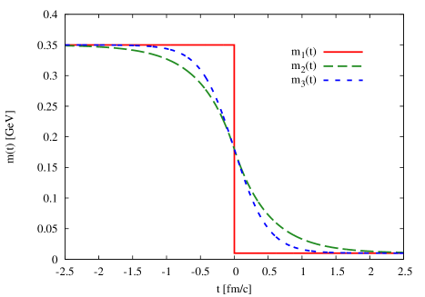
Figure 2: During the chiral phase transition, the quark/antiquark mass changes from its constituent value, $m_{c}$, to its bare value, $m_{b}$.

It has been shown in Greiner (1995, 1996) that the asymptotic occupation numbers are very sensitive to the order of differentiability of the considered mass parametrization, $m(t)$. For the case of an instantaneous mass shift described by (92a), the equation of motion (31) for the positive- and negative-energy wave function is solved analytically with the ansatz

$$\psi_{\vec{p},s,\uparrow}(x) = \begin{cases}\psi^{c}_{\vec{p},s,\uparrow}(x)&\mbox{for}\quad t<0\ ,\\ \alpha_{\vec{p},s}\psi^{b}_{\vec{p},s,\uparrow}(x)+\beta_{\vec{p},s}\psi^{b}_{\vec{p},s,\downarrow}(x)&\mbox{for}\quad t\geq 0\ ,\end{cases}$$ (93a)

$$\psi_{\vec{p},s,\downarrow}(x) = \begin{cases}\psi^{c}_{\vec{p},s,\downarrow}(x)&\mbox{for}\quad t<0\ ,\\ \gamma_{\vec{p},s}\psi^{b}_{\vec{p},s,\downarrow}(x)+\delta_{\vec{p},s}\psi^{b}_{\vec{p},s,\uparrow}(x)&\mbox{for}\quad t\geq 0\ .\end{cases}$$ (93b)

For $t<0$, $\psi_{\vec{p},s,\uparrow}(x)$ and $\psi_{\vec{p},s,\downarrow}(x)$ describe positive- and negative-energy states of mass $m_{c}$, respectively, whereas they turn into superpositions of positive- and negative-energy states of mass $m_{b}$ for $t\geq 0$. From the continuity condition

$$\psi_{\vec{p},s,\uparrow\downarrow}(\vec{x},0^{-})=\psi_{\vec{p},s,\uparrow\downarrow}(\vec{x},0^{+})\ ,$$ (94)

we obtain

$$\alpha_{\vec{p},s}= \gamma_{\vec{p},s} =\cos\varphi^{b}_{\vec{p}}\cos\varphi^{c}_{\vec{p}}+\sin\varphi^{b}_{\vec{p}}\sin\varphi^{c}_{\vec{p}}\ ,$$ (95a)

$$\beta_{\vec{p},s}= -\delta_{\vec{p},s} =\sin\varphi^{b}_{\vec{p}}\cos\varphi^{c}_{\vec{p}}-\cos\varphi^{b}_{\vec{p}}\sin\varphi^{c}_{\vec{p}}\ .$$ (95b)

As the coefficients $\alpha_{\vec{p},s}$ and $\beta_{\vec{p},s}$ do not explicitly depend on the spin, $s$, this index will be omitted from now on. The occupation numbers thus read

$$\begin{split}\frac{\text{d}^{6}n_{q\bar{q}}(t)}{\text{d}^{3}x\text{d}^{3}p}&=\frac{2\beta^{2}_{\vec{p}}}{(2\pi)^{3}}\\ &=\frac{1}{(2\pi)^{3}}\left[1-\frac{p^{2}+m_{b}m_{c}}{E^{b}_{\vec{p}}E^{c}_{\vec{p}}}\right]\end{split}$$ (96)

for $t>0$, whereas they vanish for $t<0$. For $p\gg m_{b},m_{c}$, the expression (96) can be approximated as

$$\frac{\text{d}^{6}n_{q\bar{q}}(t)}{\text{d}^{3}x\text{d}^{3}p}\simeq\frac{(m_{c}-m_{b})^{2}}{(2\pi)^{3}2p^{2}}+\mathcal{O}(1/p^{4})\ ,$$ (97)

which means that the total particle number density and the total energy density of the fermionic sector are linearly and quadratically divergent, respectively.

This artifact can be removed if the mass shift is assumed to take place over a finite time interval, $\tau$. In this case, the occupation numbers are obtained by solving (36) numerically for the negative-energy wavefunction parameters, $\alpha_{\vec{p}¸\downarrow,}(t)$ and $\beta_{\vec{p}¸\downarrow}(t)$, which are then inserted into (90). Fig. 3 compares the asymptotic particle spectra for the different mass parameterizations, $m_{i}(t)$.

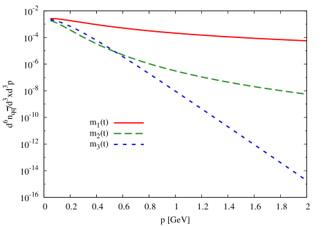
Figure 3: Asymptotic particle spectra for the different mass parameterizations given in Eqs. (92). The decay behavior is highly sensitive to the order of differentiability of $m(t)$. Both for $m_{2}(t)$ and $m_{3}(t)$, we have chosen $\tau=1.0$ fm/c.

Analogously to Greiner (1995, 1996), we find that if we turn from $m_{1}(t)$ to $m_{2}(t)$, which is continuously differentiable once, the occupation numbers decay $\propto 1/p^{6}$ and are hence suppressed relative to the case with the instantaneous transition. Moreover, if we turn from $m_{2}(t)$ to $m_{3}(t)$, which is continuously differentiable infinitely many times, the occupation numbers are further suppressed to an exponential decay. In the limit $\tau\rightarrow 0$, both $m_{2}(t)$ and $m_{3}(t)$ reproduce expression (96), which is depicted in Fig. 4.

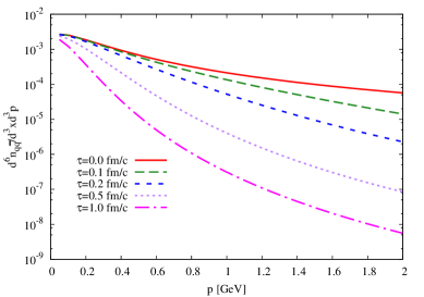
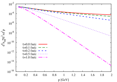
Figure 4: Asymptotic particle spectra for $m_{2}(t)$ (left panel) and $m_{3}(t)$ (right panel) for different transition times, $\tau$. In each case, the suppression at large $p$ with respect to an instantaneous mass shift is the stronger the more slowly ($\tau$ increasing) the mass shift is assumed to take place. As expected, both parameterizations reproduce expression (96) in the limit $\tau\rightarrow 0$.

We shall briefly explain how the sensitivity of the asymptotic occupation numbers on the mass parametrization, $m_{i}(t)$, comes about. For this purpose, we consider the Bogolyubov parameters in terms of negative-energy wavefunction parameters,

$$\xi^{*}_{\vec{p},s}(t) = \sqrt{\frac{E_{\vec{p}}(t)-m(t)}{2E_{\vec{p}}(t)}}\alpha^{*}_{\vec{p},\downarrow}(t)-\sqrt{\frac{E_{\vec{p}}(t)+m(t)}{2E_{\vec{p}}(t)}}\beta^{*}_{\vec{p},\downarrow}(t)\ ,$$ (98a)

$$\eta_{\vec{p},s}(t) = \sqrt{\frac{E_{\vec{p}}(t)+m(t)}{2E_{\vec{p}}(t)}}\alpha_{\vec{p},\downarrow}(t)+\sqrt{\frac{E_{\vec{p}}(t)-m(t)}{2E_{\vec{p}}(t)}}\beta_{\vec{p},\downarrow}(t)\ ,$$ (98b)

with (98a) following from (85a) and (39). We do not take into account the phase factor, $\text{e}^{\text{i}E_{\vec{p}}(t)t}$, as it drops out when taking the absolute square of (98b) to obtain the Bogolyubov particle number density (74). It follows from (36) that $\xi^{*}_{\vec{p},s}(t)$ and $\eta_{\vec{p},s}(t)$ then obey the equations of motion,

$$\text{i}\partial_{t}\xi^{*}_{\vec{p},s}(t) = -\text{i}\frac{p\dot{m}(t)}{2E^{2}_{\vec{p}}(t)}\eta_{\vec{p},s}(t)-E_{\vec{p}}(t)\xi^{*}_{\vec{p},s}(t)\ ,$$ (99a)

$$\text{i}\partial_{t}\eta_{\vec{p},s}(t) = \text{i}\frac{p\dot{m}(t)}{2E^{2}_{\vec{p}}(t)}\xi^{*}_{\vec{p},s}(t)+E_{\vec{p}}(t)\eta_{\vec{p},s}(t)\ .$$ (99b)

In the limit $p\gg m(t)$, these equations of motion are approximately solved by

$$\begin{split}\xi^{*}_{\vec{p},s}(t)&=\text{e}^{\text{i}pt}\ ,\\ \eta_{\vec{p},s}(t)&=\frac{\text{e}^{-\text{i}pt}}{2p}\int_{t_{0}}^{t}\text{d}t^{\prime}\dot{m}(t^{\prime})\text{e}^{2\text{i}pt^{\prime}}\ .\end{split}$$ (100)

Hence, the Bogolyubov particle number density in that domain reads

$$\frac{\text{d}^{6}n_{q\bar{q}}(t)}{\text{d}^{3}x\text{d}^{3}p}\simeq\frac{(m_{c}-m_{b})^{2}}{(2\pi)^{3}2p^{2}}\left|\int_{-\infty}^{t}\text{d}t^{\prime}\chi(t^{\prime})\text{e}^{2\text{i}pt^{\prime}}\right|^{2}\ ,$$ (101)

where we have formally introduced $\chi(t)$ by means of the relation $\dot{m}(t)=\chi(t)(m_{c}-m_{b})$ and taken $t_{0}\rightarrow-\infty$ since $\dot{m}(t)\rightarrow 0$ for $t\rightarrow\pm\infty$. In particular, in the asymptotic limit, $t\rightarrow\infty$, we have for the quark/antiquark occupation numbers,

$$\left.\frac{\text{d}^{6}n_{q\bar{q}}(t)}{\text{d}^{3}x\text{d}^{3}p}\right|_{t\rightarrow\infty}\simeq\frac{(m_{c}-m_{b})^{2}}{(2\pi)^{3}2p^{2}}\left|\int_{-\infty}^{\infty}\text{d}t^{\prime}\chi(t^{\prime})\text{e}^{2\text{i}pt^{\prime}}\right|^{2}\ .$$ (102)

So for a mass shift over a finite time interval, $\tau$, (97) is effectively modulated with the absolute square of the Fourier transform of $\chi(t)$ from $t$ to $2p$. So the particle numbers for $p\gg m_{b},m_{c}$ are suppressed by an additional factor of $1/p^{2}$ each time the order of differentiability of $m(t)$ is increased by one. In particular, for $m(t)=m_{2}(t)$ we have

$$\left.\frac{\text{d}^{6}n_{q\bar{q}}(t)}{\text{d}^{3}x\text{d}^{3}p}\right|_{t\rightarrow\infty}\simeq\frac{(m_{c}-m_{b})^{2}}{(2\pi)^{3}2p^{2}}\frac{1}{(1+p^{2}\tau^{2})^{2}}\ .$$ (103)

As a next step, we extend the investigations in Greiner (1995, 1996) to the time dependence of the occupation numbers. Fig. 5 shows the time evolution of (90) for different momentum modes.

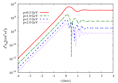
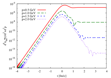
Figure 5: Time dependence of occupation numbers for $m_{2}(t)$ (left panel) and $m_{3}(t)$ (right panel) for $\tau=1.0$ fm/c. For large values of $p$, they exhibit an ’overshoot’ over their asymptotic value around $t=0$, which is particularly distinctive for $m_{3}(t)$.

Here we see that for hard momentum modes, the occupation numbers exhibit a strong ‘overshoot’ over their asymptotic values by several orders of magnitude in the region of strong mass gradients. This means that the particle spectra exhibit their decay behavior characteristic for the order of differentiability of $m(t)$ only in the limit $t\rightarrow\infty$, which is depicted in Fig. 6.

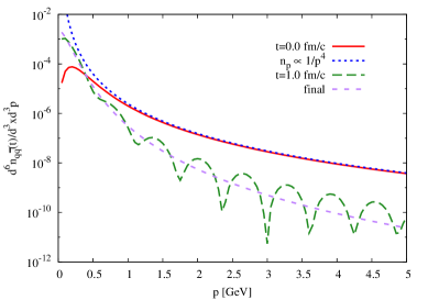
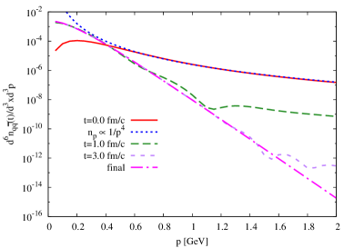
Figure 6: Particle spectra for $m_{2}(t)$ (left panel) and $m_{3}(t)$ (right panel) at different times, $t$, for a transition time of $\tau=1.0$ fm/c. For both parameterizations, the characteristic decay behavior only emerges for $t\rightarrow\infty$, whereas one encounters a decay behavior $\propto 1/p^{4}$ for large $p$ around $t=0$.

At finite times, however, the particle spectra decay as $1/p^{4}$ both for $m_{2}(t)$ and for $m_{3}(t)$ for $p\gg m_{b},m_{c}$. This can be understood by taking into account that at intermediate times the time integral in (101) runs from $-\infty$ to $t$, so that one effectively carries out a Fourier transform over a discontinuous function. Hence, expression (90) picks up an additional factor of $1/p^{2}$ compared to the case of an instantaneous mass shift. This implies that at finite times, $t$, the total particle number density is finite whereas the total energy density features a logarithmic divergence. This is depicted in Fig. 7 showing its time evolution with the loop integral entering (82) being regulated by a cutoff at different values of $p=\Lambda_{C}$.

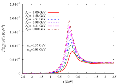
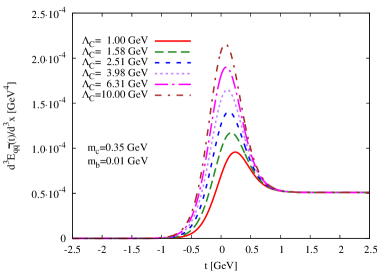
Figure 7: Time evolution of the total energy density for $m(t)=m_{2}(t)$ (left panel) and $m(t)=m_{3}(t)$ (right panel) for $\tau=1.0$ fm/c. It features a logarithmic divergence in the regions of strong mass gradients, which disappears again as soon as the quark/antiquark mass has reached its final bare value, $m_{b}$.

The considered values of $\Lambda_{C}$ follow an exponentially increasing sequence given by

$$\Lambda_{C}(i)=\Lambda_{1}\text{e}^{0.2\ln{\frac{\Lambda_{2}}{\Lambda_{1}}}i}\ ,$$

with $\Lambda_{1}=1$ GeV, $\Lambda_{2}=10$ GeV, and $i$ going from $0$ to $5$. This choice is such that in the region of strong mass gradients, the total energy density always increases by a constant amount for consecutive $\Lambda_{C}(i)$, which reflects the logarithmic divergence of energy density (82). This divergence, however, only shows up in regions of strong mass gradients and disappears again as soon as the fermion mass has reached its final value. Among other things, this can also be inferred from Fig. 7.

For $m(t)=m_{2}(t)$ and $t>0$, the particle spectrum does not decay strictly monotonously for $p\gg m_{b},m_{c}$, but instead exhibits an oscillatory behavior. This can be understood by taking into account that

$$\left|\int_{-\infty}^{t}\text{d}t^{\prime}\chi(t^{\prime})e^{2\text{i}pt^{\prime}}\right|^{2}= \frac{e^{-2t/\tau}}{4(1+p^{2}\tau^{2})}+\frac{1-e^{-2t/\tau}\left(\cos{2pt}-p\tau\sin{2pt}\right)}{(1+p^{2}\tau^{2})^{2}}$$ (104)

for $t\geq 0$ from which the oscillatory behavior of (101) in $p$ at positive times becomes apparent. For $t\rightarrow\infty$, the oscillating terms disappear so that the asymptotic particle spectrum shows a strictly monotonous decay again.

For the sake of completeness, we also consider the case where the fermion mass first undergoes a change from its constituent value, $m_{c}$, to its bare value, $m_{b}$, and then again back to its constituent value, $m_{c}$, after a certain period of time, $\tau_{L}$, to simulate the temporary restoration of chiral symmetry during a heavy-ion collision. Again we consider different mass parameterizations,

$$\tilde{m}_{1}(t)=\frac{m_{c}+m_{b}}{2}-\frac{m_{c}-m_{b}}{2} \text{sign}\left(\frac{\tau_{L}^{2}}{4}-t^{2}\right)\ ,$$ (105a)

$$\tilde{m}_{2}(t)=\frac{m_{c}+m_{b}}{2}-\frac{m_{c}-m_{b}}{2} \mbox{sign}\left(t+\frac{\tau_{L}}{2}\right)\left(1-\text{e}^{-|2t+\tau_{L}|/\tau}\right)$$

$$\times \mbox{sign}\left(\frac{\tau_{L}}{2}-t\right)\left(1-\text{e}^{-|2t-\tau_{L}|/\tau}\right)\ ,$$ (105b)

$$\tilde{m}_{3}(t)=\frac{m_{c}+m_{b}}{2}-\frac{m_{c}-m_{b}}{2} \mbox{tanh}\left(\frac{2t+\tau_{L}}{\tau}\right)\mbox{tanh}\left(\frac{\tau_{L}-2t}{\tau}\right)\ .$$ (105c)

Here $\tau_{L}$ denotes the lifetime of the quark-gluon plasma during which the chiral symmetry is restored. For our numerical investigations, we choose $\tau_{L}=4$ fm/c for which (105a)-(105c) are depicted in Fig. 8.

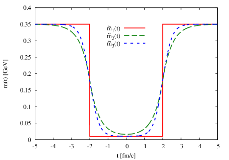
Figure 8: The mass is first changed from $m_{c}$ to $m_{b}$ and then back to $m_{c}$ again to simulate the temporary restoration of chiral symmetry.

For the case of $\tilde{m}_{1}(t)$, where both mass shifts are assumed to take place instantaneously, the Dirac equation (31) is solved with an ansatz similar to (93):

$$\psi_{\vec{p},s,\uparrow}(x) = \begin{cases}\psi^{c}_{\vec{p},s,\uparrow}(x)&\mbox{for}\quad t<-\tau_{L}/2\ ,\\ \alpha_{\vec{p}}\psi^{b}_{\vec{p},s,\uparrow}(x)+\beta_{\vec{p}}\psi^{b}_{\vec{p},s,\downarrow}(x)&\mbox{for}\quad-\tau_{L}/2\leq t\leq\tau_{L}/2\ ,\\ \tilde{\alpha}_{\vec{p}}\psi^{c}_{\vec{p},s,\uparrow}(x)+\tilde{\beta}_{\vec{p}}\psi^{c}_{\vec{p},s,\downarrow}(x)&\mbox{for}\quad t>\tau_{L}/2\ ,\end{cases}$$ (106a)

$$\psi_{\vec{p},s,\downarrow}(x) = \begin{cases}\psi^{c}_{\vec{p},s,\downarrow}(x)&\mbox{for}\quad t<-\tau_{L}/2\ ,\\ \gamma_{\vec{p}}\psi^{b}_{\vec{p},s,\downarrow}(x)+\delta_{\vec{p}}\psi^{b}_{\vec{p},s,\uparrow}(x)&\mbox{for}\quad-\tau_{L}/2\leq t\leq\tau_{L}/2\ ,\\ \tilde{\gamma}_{\vec{p}}\psi^{c}_{\vec{p},s,\downarrow}(x)+\tilde{\delta}_{\vec{p}}\psi^{c}_{\vec{p},s,\uparrow}(x)&\mbox{for}\quad t>\tau_{L}/2\ .\end{cases}$$ (106b)

The successive application of the continuity conditions $\psi_{\vec{p},s,\uparrow\downarrow}(\vec{x},-\tau/2^{-})=\psi_{\vec{p},s,\uparrow\downarrow}(\vec{x},-\tau/2^{+})$ and $\psi_{\vec{p},s,\uparrow\downarrow}(\vec{x},\tau/2^{-})=\psi_{\vec{p},s,\uparrow\downarrow}(\vec{x},\tau/2^{+})$ leads to

$$\alpha_{\vec{p}} = \gamma^{*}_{\vec{p}}$$ (107a)

$$= \text{e}^{\text{i}(E^{c}_{\vec{p}}-E^{b}_{\vec{p}})\tau_{L}/2}\left(\cos\varphi^{b}_{\vec{p}}\cos\varphi^{c}_{\vec{p}}+\sin\varphi^{b}_{\vec{p}}\sin\varphi^{c}_{\vec{p}}\right)\ ,$$

$$\beta_{\vec{p}} = -\delta^{*}_{\vec{p}}$$ (107b)

$$= \text{e}^{\text{i}(E^{c}_{\vec{p}}+E^{b}_{\vec{p}})\tau_{L}/2}\left(\sin\varphi^{b}_{\vec{p}}\cos\varphi^{c}_{\vec{p}}-\cos\varphi^{b}_{\vec{p}}\sin\varphi^{c}_{\vec{p}}\right)\ ,$$

$$\tilde{\alpha}_{\vec{p}} = \tilde{\gamma}_{\vec{p}}^{*}$$ (107c)

$$= \alpha^{2}_{\vec{p}}+\beta^{2}_{\vec{p}}\ ,$$

$$\tilde{\beta}_{\vec{p}} = -\tilde{\delta}_{\vec{p}}^{*}$$ (107d)

$$= 2\text{i}\mbox{Im}\left\{\alpha^{*}_{\vec{p}}\beta_{\vec{p}}\right\}\ .$$

Hence, for $-\tau_{L}/2\leq t\leq\tau_{L}/2$, the occupations numbers are given by (96) whereas for $t>\tau_{L}/2$ we have

$$\frac{\text{d}^{6}n_{q\bar{q}}(t)}{\text{d}^{3}x\text{d}^{3}p} = \frac{2}{(2\pi)^{3}}\left|\tilde{\beta}_{\vec{p}}\right|^{2}$$ (108)

$$= \frac{2}{(2\pi)^{3}}\left[1-\left(\frac{p^{2}+m_{b}m_{c}}{E^{b}_{\vec{p}}E^{c}_{\vec{p}}}\right)^{2}\right]\sin^{2}(E^{b}_{\vec{p}}\tau_{L})$$

$$\simeq 2\frac{(m_{c}-m_{b})^{2}}{(2\pi)^{3}p^{2}}\sin^{2}(p\tau_{L})\quad\mbox{for}\quad p\gg m_{b},m_{c}.$$

Consequently, for given momentum, $\vec{p}$, the final occupation number is highly sensitive to $\tau_{L}$ and becomes maximal if the condition

$$E^{b}_{\vec{p}}\tau_{L}=\frac{2n+1}{2}\pi\quad\text{with}\quad n\in\mathbb{N}_{0}\ ,$$

is satisfied. Comparing the asymptotic particle number density for different mass parameterizations $\tilde{m}(t)$, we observe the same sensitivity on the respective order of differentiability for large $p$ as we did in the first scenario. This is depicted in Fig. 9 and follows immediately from expression (101).

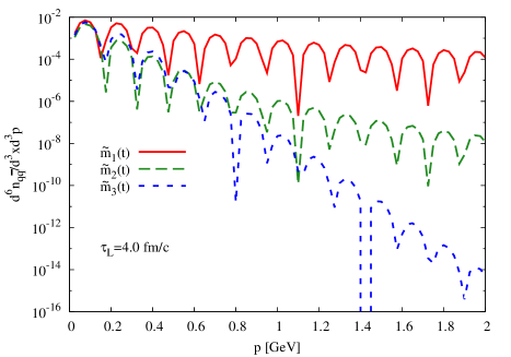
Figure 9: Asymptotic particle spectra for the different mass parameterizations in Eqs. (105). Analogously to the first scenario where the mass is not restored to its initial value, the decay behavior is highly sensitive to the order of differentiability of $\tilde{m}(t)$. Both for $\tilde{m}_{2}(t)$ and for $\tilde{m}_{3}(t)$ we have chosen $\tau=1.0\;\mathrm{fm}/c$.

Similarly to the first case, both (105b) and (105c) reproduce the particle spectrum of (105a) in the limit $\tau\rightarrow 0$, which is shown in figure 10.

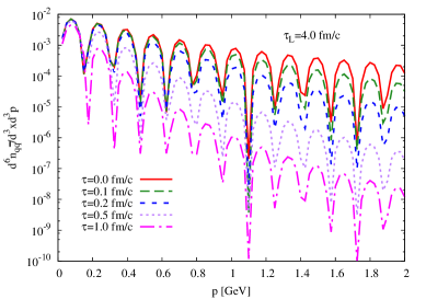
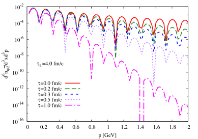
Figure 10: Asymptotic particle spectra for $\tilde{m}_{2}(t)$ (left panel) and $\tilde{m}_{3}(t)$ (right panel) for different values of $\tau$. Analogously to the first scenario, the suppression at large $p$ compared to the instantaneous case is the stronger the more slowly ($\tau$ increasing) both mass changes are assumed to take place. As it must be, expression (108) is reproduced in the limit $\tau\rightarrow 0$ for both parameterizations.

Fig. 11 shows the time evolution of the particle number density for $\tilde{m}_{3}(t)$ with $\tau=1\;\mathrm{fm}/c$ and $\tau_{L}=8\;\mathrm{fm}/c$. As it should be, the time dependence in the second scenario is the same as in the first one until we start changing the fermion mass back to its initial constituent value, $m_{c}$. Hence, the occupation numbers first saturate at the same value as they did within the first scenario. As soon as a second mass gradient shows up, they are again changing by several orders of magnitude before they saturate at their final asymptotic value, which is usually different from the first one.

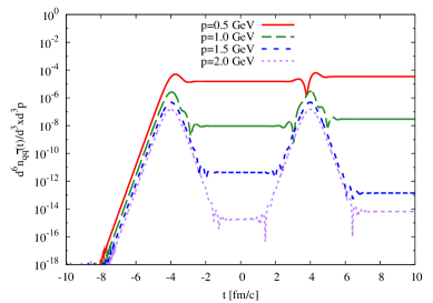
Figure 11: Time evolution of the particle number density for $\tilde{m}_{3}(t)$ with $\tau=1.0\;\mathrm{fm}/c$ and $\tau_{L}=8.0\;\mathrm{fm}/c$. They are again changing by several orders of magnitude when the mass is being restored to its initial constituent value, $m_{c}$.

Such a behavior follows immediately from expression (101). At times when the fermion mass is at its bare value, $m_{b}$, the integral entering it effectively represents a full Fourier transform over an at least continuous function while we again encounter a Fourier transform over a discontinuous function again when the fermion mass is being changed back to its constituent value, $m_{c}$.

For completeness, we still have to investigate in more detail how the occupation numbers are modified if the quark mass is changed back to its initial value, $m_{c}$. For this purpose, we take into account that our mass parametrization (92) and (105) can be written in the general form

$$m(t) = \frac{m_{c}+m_{b}}{2}-\frac{m_{c}-m_{b}}{2}f(t)\ ,$$ (109a)

$$\tilde{m}(t) = \frac{m_{c}+m_{b}}{2}-\frac{m_{c}-m_{b}}{2}f\left(t+\frac{\tau_{L}}{2}\right)f\left(\frac{\tau_{L}}{2}-t\right)\ ,$$ (109b)

with $f(t)$ increasing monotonously from $-1$ to $1$ and fulfilling the condition $f(-t)=-f(t)$ (odd under time inversion). Hence, we have

$$\tilde{\chi}(t)=f\left(\frac{\tau_{L}}{2}-t\right)\chi\left(\frac{\tau_{L}}{2}+t\right)-\chi\left(\frac{\tau_{L}}{2}-t\right)f\left(\frac{\tau_{L}}{2}+t\right)\ .$$ (110)

The Fourier transform of (110) from $t$ to $2p$ is given by

$$\int_{-\infty}^{\infty}\text{d}t^{\prime}\tilde{\chi}(t^{\prime})\text{e}^{2\text{i}pt^{\prime}}=2\text{i}\operatorname{Im}\left\{\text{e}^{-\text{i}p\tau_{L}}\int_{-\infty}^{\infty}\text{d}t^{\prime}f\left(\tau_{L}-t^{\prime}\right)\chi(t^{\prime})\text{e}^{2\text{i}pt^{\prime}}\right\}\ .$$ (111)

Thus, unlike the case where the fermion mass is changed instantaneously, the occupation numbers for $p\gg m_{b},m_{c}$ in the second scenario are generally different from those in the first scenario multiplied by a factor of $4\sin^{2}(p\tau_{L})$. Nevertheless, if $\tau_{L}$ is significantly larger than $\tau$, we have $f(\tau_{L}-t)\approx 1$ for those times, $t$, where $\chi(t)$ is significantly different from zero. We can hence approximate

$$\int_{-\infty}^{\infty}\text{d}t^{\prime}\tilde{\chi}(t^{\prime})\text{e}^{2\text{i}pt^{\prime}}\approx-2\text{i}\sin p_{L}\tau\int_{-\infty}^{\infty}\text{d}t^{\prime}\chi(t^{\prime})\text{e}^{2\text{i}pt^{\prime}},$$ (112)

where we have also taken into account that $\chi(-t)=\chi(t)$. The latter follows immediately from $f(-t)=-f(t)$. Hence, for $\tau\ll\tau_{L}$, the asymptotic occupation numbers for hard quark-antiquark pairs are given by

$$\left.\frac{\text{d}^{6}n_{q\bar{q}}(t)}{\text{d}^{3}x\text{d}^{3}p}\right|_{t\rightarrow\infty}=2\frac{(m_{b}-m_{c})^{2}}{(2\pi)^{3}p^{2}}\left|\int_{-\infty}^{\infty}\text{d}t^{\prime}\chi(t^{\prime})\text{e}^{2\text{i}pt^{\prime}}\right|^{2}\sin^{2}(p\tau_{L})\ ,$$ (113)

which just corresponds to (101) modified by a factor of $4\sin^{2}(p\tau_{L})$. This is illustrated in Fig. 12 for the asymptotic particle spectrum of $\tilde{m}_{2}(t)$, where the dotted line represents the spectrum for $m_{2}(t)$ multiplied by $4\sin^{2}(p\tau_{L})$.

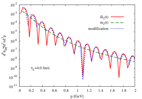
Figure 12: Comparison of asymptotic particle spectra for $\tilde{m}_{2}(t)$ and $m_{2}(t)$ for $\tau=1.0$ fm/c. For large values of $p$, the asymptotic occupation numbers of $\tilde{m}_{2}(t)$ essentially differ from those of $m_{2}(t)$ by a modification factor of $4\sin^{2}{p\tau_{L}}$.

To summarize, we have found that the occupation numbers in the asymptotic limit show a strong dependence on the ‘smoothness’ of the considered mass parametrization, $m(t)$. For the case of an instantaneous mass shift, they scale $\propto(m_{c}-m_{b})^{2}/p^{2}$ for $p\gg m_{c},m_{b}$ which means that the total number density is linearly divergent. This artifact is removed if the mass shift takes place over a finite time interval, $\tau$. In particular, the quark/antiquark occupation numbers at $p\gg m_{c},m_{b}$ and $p\gg 1/\tau$ scale $\propto(m_{c}-m_{b})^{2}/p^{6}\tau^{4}$ for $m_{2}(t)$ (continuously differentiable once) and are suppressed even further to an exponential decay for $m_{3}(t)$ (continuously differentiable infinitely many times).

Our investigations have shown that the pathological scaling behavior for an instantaneous mass shift essentially results from high-momentum Fourier components. These components are suppressed for mass shifts over a finite time interval such that the scaling behavior of the quark/antiquark occupation numbers becomes physically reasonable. A very similar effect occurs when considering back-to-back particle-antiparticle correlations in high energy nuclear collisions for mass parameterizations with different order of differentiability Vourdas and Weiner (1988); Razumov and Weiner (1995); Asakawa and Csorgo (1996); Asakawa et al. (1999); Dudek and Padula (2010); Knoll (2011) .

Furthermore, if the quark mass is changed back from its bare value, $m_{b}$, to its constituent value, $m_{c}$, the lifetime of the chirally restored phase enters the asymptotic occupations numbers at large $p\gg m_{b},m_{c}$ in the form of a factor of $4\sin^{2}(p\tau_{L})$ if $\tau\ll\tau_{L}$. From the semiclassical point of view, the oscillations in the particle spectra emerging from this factor correspond to a multiple scattering of the quarks/antiquarks at both mass gradients.

At intermediate times, however, the quark/antiquark occupation numbers decay $\propto 1/p^{4}$ for large $p$ in regions of strong mass gradients. This, in turn, leads to a transient logarithmic divergence in the total energy density of the quarks and antiquarks. At first sight such a divergence might be disturbing. We stress, however, that only the asymptotic energy density, i.e. for $t\to+\infty$, constitutes an observable in the sense of S-matrix theory, as the interpretation of (74) as quark/antiquark occupation numbers is only justified for asymptotic times where $\dot{m}(t)=0$. The reason is that the dispersion relation (80) then actually characterizes free and thus detectable particles wheres it only describes quasiparticles for $\dot{m}(t)\neq 0$ Filatov et al. (2008). Moreover, the asymptotic value does not show any divergence as long as the mass shift is smooth enough, which is a physically reasonable condition. Yet, there is one more twist in this argument when we proceed to the photon production. Photons are produced (and, in principle, leave the system) at any instant of time. Thus one might suspect that the tremendously large intermediate fermion numbers leave their imprint on the number of emitted photons. It is conceivable that the asymptotic number of photons, which is an accumulation over the whole time history, becomes large or even diverges just because there have been very many fermionic emitters at intermediate times. We will see in the following that this is not the case. It is important to understand that the disappearance of the large fermion numbers is not a damping effect, but a quantum mechanical interference effect. Collisions between the fermions, which would provide a loss rate, i.e. damping, are not included in our approach. On the other hand, the full quantum effects are retained, which can lead to interference patterns that are unintuitive from a classical point of view. This applies in particular to quantities which are not observable anyhow like, for instance, the number of fermions at finite times. In the same way the asymptotic photon number can turn out to be reasonably small in spite of the fact that the emitted photons seem to pile up during the whole history of the process.

IV Photon production

We now turn to our investigations on photon production. As it has been shown in the previous section, the asymptotic quark/antiquark occupation numbers exhibit a strong sensitivity to the order of differentiability of the time dependence of the mass, $m(t)$. In particular, they are rendered integrable in the ultraviolet domain, if the mass shift is assumed to take place over a finite time interval, $\tau$. We now investigate whether the resulting photon spectra exhibit a similar sensitivity and if the model of chiral photon production is accordingly suitable to describe finite-lifetime effects on the photon emission from a quark-gluon plasma. As one lesson from section III we recall that only the asymptotic particle numbers constitute observables Filatov et al. (2008), while quantities defined by the analogous expressions with interpolating fields have no definite interpretation as particle numbers. Thus, in the following we concentrate on the asymptotic photon numbers (62).

IV.1 Instantaneous mass shift

First, we consider photon production for an instantaneous mass shift at $t=0$ as this special case still allows for an almost complete analytical treatment. In particular, the individual contributions to the photon yield allow for an interpretation as first-order QED processes and their interference among each other.

On the other hand, we show that the assumption of an instantaneous mass shift comes along with essentially three unphysical artifacts. In section IV.1.1, we calculate the individual contributions to the photon yield (62). Thereby, we will demonstrate that the overall loop integral entering (62) features a linear divergence caused by the decay behavior of the quark/antiquark occupation numbers (96) for $p\gg m_{b},m_{c}$. We regulate this divergence by cutting off the loop integral at $p=\Lambda_{C}$.

We will see in section IV.1.2 that then the resulting asymptotic photon spectra decay as $1/\omega^{3}_{\vec{k}}$, with $\omega_{\vec{k}}$ denoting the photon energy (23), in the ultraviolet domain for given value of $\Lambda_{C}$. The total number density and the total energy density of the emitted photons are hence logarithmically and linearly divergent, respectively.

Finally, as we mention at the end of section IV.1.2 and discuss in greater detail in appendix F, another problem appears in the limit $m_{b}\rightarrow 0$. In that limit, the loop integral over the contributions describing quark and antiquark bremsstrahlung and quark-antiquark-pair annihilation into a photon feature a collinear and an anticollinear singularity, respectively.

IV.1.1 Evaluation of contributions to the photon yield

To evaluate the contributions to the photon yield for an instantaneous mass shift, we first undo the contraction

$$\text{i}\Pi^{<}_{T}(\vec{k},t_{1},t_{2})=\gamma^{\mu\nu}(k)\Pi^{<}_{\nu\mu}(\vec{k},t_{1},t_{2})\ ,$$

and express the photon self-energy in terms of positive and negative energy wavefunctions, i.e.,

$$\text{i}\Pi^{<}_{\mu\nu}(\vec{k},t_{1},t_{2})= e^{2}\sum_{r,s}\int\frac{\text{d}^{3}p}{(2\pi)^{3}}\left[\bar{\psi}^{{}^{\prime}}_{\vec{p},r,\uparrow}(t_{1})\gamma_{\mu}\psi^{{}^{\prime}}_{\vec{p}+\vec{k},s,\downarrow}(t_{1})\right]\cdot\left[\bar{\psi}^{{}^{\prime}}_{\vec{p}+\vec{k},s,\downarrow}(t_{2})\gamma_{\nu}\psi^{{}^{\prime}}_{\vec{p},r,\uparrow}(t_{2})\right]$$

$$= e^{2}\sum_{r,s}\int\frac{\text{d}^{3}p}{(2\pi)^{3}}\left[\bar{\psi}^{{}^{\prime}}_{\vec{p},r,\uparrow}(t_{1})\gamma_{\mu}\psi^{{}^{\prime}}_{\vec{p}+\vec{k},s,\downarrow}(t_{1})\right]\cdot\left[\bar{\psi}^{{}^{\prime}}_{\vec{p},r,\uparrow}(t_{2})\gamma_{\nu}\psi^{{}^{\prime}}_{\vec{p}+\vec{k},s,\downarrow}(t_{2})\right]^{*}\ .$$ (114)

Upon insertion of (IV.1.1) into (62) and interchanging both time integrations with the loop integral, we can rewrite (62) as

$$2\omega_{\vec{k}}\frac{\text{d}^{6}n_{\gamma}}{\text{d}^{3}x\text{d}^{3}k}=\lim_{\varepsilon\rightarrow 0}\frac{\gamma^{\mu\nu}(k)}{(2\pi)^{3}}\sum_{r,s}\int\frac{\text{d}^{3}p}{(2\pi)^{3}}I^{\varepsilon,*}_{\mu}(\vec{p},\vec{k},r,s)I^{\varepsilon}_{\nu}(\vec{p},\vec{k},r,s)\ .$$ (115)

Here we have introduced

$$I^{\varepsilon}_{\mu}(\vec{p},\vec{k},r,s)=e\int_{-\infty}^{\infty}\underline{\text{d}t}\mbox{ }\bar{\psi}^{{}^{\prime}}_{\vec{p},r,\uparrow}(t)\gamma_{\mu}\psi^{{}^{\prime}}_{\vec{p}+\vec{k},s,\downarrow}(t)\text{e}^{\text{i}\omega_{\vec{k}}t}\ ,$$ (116)

with the underline denoting that the time integral is regulated by the convergence factor $f_{\varepsilon}(t)=\text{e}^{-\varepsilon|t|}$. Moreover, with the help of (93) and (95a), we obtain

$$\begin{split}I^{\varepsilon}_{\mu}(\vec{p},\vec{k},r,s)=e&\left[\bar{u}_{c}(\vec{p},r)\gamma_{\mu}v_{c}(\vec{p}+\vec{k},s)\frac{1}{\varepsilon+\text{i}\omega^{c}_{1}(\vec{p},\vec{k})}\right.\\ &+\alpha_{\vec{p}}\alpha_{\vec{p}+\vec{k}}\bar{u}_{b}(\vec{p},r)\gamma_{\mu}v_{b}(\vec{p}+\vec{k},s)\frac{1}{\varepsilon-\text{i}\omega^{b}_{1}(\vec{p},\vec{k})}\\ &-\alpha_{\vec{p}}\beta_{\vec{p}+\vec{k}}\bar{u}_{b}(\vec{p},r)\gamma_{\mu}u_{b}(\vec{p}+\vec{k},s)\frac{1}{\varepsilon+\text{i}\omega^{b}_{2}(\vec{p},\vec{k})}\\ &+\beta_{\vec{p}}\alpha_{\vec{p}+\vec{k}}\bar{v}_{b}(\vec{p},r)\gamma_{\mu}v_{b}(\vec{p}+\vec{k},s)\frac{1}{\varepsilon-\text{i}\omega^{b}_{3}(\vec{p},\vec{k})}\\ &\left.-\beta_{\vec{p}}\beta_{\vec{p}+\vec{k}}\bar{v}_{b}(\vec{p},r)\gamma_{\mu}u_{b}(\vec{p}+\vec{k},s)\frac{1}{\varepsilon+\text{i}\omega^{b}_{4}(\vec{p},\vec{k})}\right]\ .\end{split}$$ (117)

To keep the notation short, we have introduced the frequencies

$$\omega^{b,c}_{1}(\vec{p},\vec{k}) = E^{b,c}_{\vec{p}+\vec{k}}+E^{b,c}_{\vec{p}}+\omega_{\vec{k}}\ ,$$ (118a)

$$\omega^{b,c}_{2}(\vec{p},\vec{k}) = E^{b,c}_{\vec{p}+\vec{k}}-E^{b,c}_{\vec{p}}-\omega_{\vec{k}}\ ,$$ (118b)

$$\omega^{b,c}_{3}(\vec{p},\vec{k}) = E^{b,c}_{\vec{p}+\vec{k}}-E^{b,c}_{\vec{p}}+\omega_{\vec{k}}\ ,$$ (118c)

$$\omega^{b,c}_{4}(\vec{p},\vec{k}) = E^{b,c}_{\vec{p}+\vec{k}}+E^{b,c}_{\vec{p}}-\omega_{\vec{k}}\ .$$ (118d)

Since (118a)-(118d) are either positive or negative definite for both $m_{c}$ and $m_{b}$ taking the limit $\varepsilon\rightarrow 0$ leads to

$$\begin{split}\lim_{\varepsilon\rightarrow 0}I^{\varepsilon}_{\mu}(\vec{p},\vec{k},r,s)=I_{\mu}(\vec{p},\vec{k},r,s)=-\text{i}e&\left[\bar{u}_{c}(\vec{p},r)\gamma_{\mu}v_{c}(\vec{p}+\vec{k},s)\frac{1}{\omega^{c}_{1}(\vec{p},\vec{k})}\right.\\ &-\alpha_{\vec{p}}\alpha_{\vec{p}+\vec{k}}\bar{u}_{b}(\vec{p},r)\gamma_{\mu}v_{b}(\vec{p}+\vec{k},s)\frac{1}{\omega^{b}_{1}(\vec{p},\vec{k})}\\ &-\alpha_{\vec{p}}\beta_{\vec{p}+\vec{k}}\bar{u}_{b}(\vec{p},r)\gamma_{\mu}u_{b}(\vec{p}+\vec{k},s)\frac{1}{\omega^{b}_{2}(\vec{p},\vec{k})}\\ &-\beta_{\vec{p}}\alpha_{\vec{p}+\vec{k}}\bar{v}_{b}(\vec{p},r)\gamma_{\mu}v_{b}(\vec{p}+\vec{k},s)\frac{1}{\omega^{b}_{3}(\vec{p},\vec{k})}\\ &\left.-\beta_{\vec{p}}\beta_{\vec{p}+\vec{k}}\bar{v}_{b}(\vec{p},r)\gamma_{\mu}u_{b}(\vec{p}+\vec{k},s)\frac{1}{\omega^{b}_{4}(\vec{p},\vec{k})}\right]\ .\end{split}$$ (119)

With the help of

$$u_{c}(\vec{p},s) = \alpha_{\vec{p}}u_{b}(\vec{p},s)+\beta_{\vec{p}}v_{b}(\vec{p},s)\ ,$$ (120a)

$$v_{c}(\vec{p},s) = \alpha_{\vec{p}}v_{b}(\vec{p},s)-\beta_{\vec{p}}u_{b}(\vec{p},s)\ ,$$ (120b)

we can rewrite (119) in the following more compact form:

$$\begin{split}I_{\mu}(\vec{p},\vec{k},r,s)=\text{i}e&\left[\alpha_{\vec{p}}\alpha_{\vec{p}+\vec{k}}\bar{u}_{b}(\vec{p},r)\gamma_{\mu}v_{b}(\vec{p}+\vec{k},s)\left(\frac{1}{\omega^{b}_{1}(\vec{p},\vec{k})}-\frac{1}{\omega^{c}_{1}(\vec{p},\vec{k})}\right)\right.\\ &+\alpha_{\vec{p}}\beta_{\vec{p}+\vec{k}}\bar{u}_{b}(\vec{p},r)\gamma_{\mu}u_{b}(\vec{p}+\vec{k},s)\left(\frac{1}{\omega^{b}_{2}(\vec{p},\vec{k})}+\frac{1}{\omega^{c}_{1}(\vec{p},\vec{k})}\right)\\ &+\beta_{\vec{p}}\alpha_{\vec{p}+\vec{k}}\bar{v}_{b}(\vec{p},r)\gamma_{\mu}v_{b}(\vec{p}+\vec{k},s)\left(\frac{1}{\omega^{b}_{3}(\vec{p},\vec{k})}-\frac{1}{\omega^{c}_{1}(\vec{p},\vec{k})}\right)\\ &\left.+\beta_{\vec{p}}\alpha_{\vec{p}+\vec{k}}\bar{v}_{b}(\vec{p},r)\gamma_{\mu}u_{b}(\vec{p}+\vec{k},s)\left(\frac{1}{\omega^{b}_{4}(\vec{p},\vec{k})}+\frac{1}{\omega^{c}_{1}(\vec{p},\vec{k})}\right)\right]\ .\end{split}$$ (121)

Since we have $\alpha_{\vec{p}}\rightarrow 1$ and $\beta_{p}\rightarrow 0$ for $m_{b}\rightarrow m_{c}$, expression (121) vanishes in this case and we will have no photon production, as it should be. Taking a closer look at the spinor structure of the particular contributions to (121) allows us to interpret them as first-order QED-transition amplitudes. It is hence convenient to split up (121) as

$$I_{\mu}(\vec{p},\vec{k},r,s) = \sum_{i=1}^{4}I^{i}_{\mu}(\vec{p},\vec{k},r,s)\ ,$$ (122a)

$$I^{1}_{\mu}(\vec{p},\vec{k},r,s) = \text{i}e\alpha_{\vec{p}}\alpha_{\vec{p}+\vec{k}}\bar{u}_{b}(\vec{p},r)\gamma_{\mu}v_{b}(\vec{p}+\vec{k},s)\left(\frac{1}{\omega^{b}_{1}(\vec{p},\vec{k})}-\frac{1}{\omega^{c}_{1}(\vec{p},\vec{k})}\right)\ ,$$ (122b)

$$I^{2}_{\mu}(\vec{p},\vec{k},r,s) = \text{i}e\alpha_{\vec{p}}\beta_{\vec{p}+\vec{k}}\bar{u}_{b}(\vec{p},r)\gamma_{\mu}u_{b}(\vec{p}+\vec{k},s)\left(\frac{1}{\omega^{b}_{2}(\vec{p},\vec{k})}+\frac{1}{\omega^{c}_{1}(\vec{p},\vec{k})}\right)\ ,$$ (122c)

$$I^{3}_{\mu}(\vec{p},\vec{k},r,s) = \text{i}e\beta_{\vec{p}}\alpha_{\vec{p}+\vec{k}}\bar{v}_{b}(\vec{p},r)\gamma_{\mu}v_{b}(\vec{p}+\vec{k},s)\left(\frac{1}{\omega^{b}_{3}(\vec{p},\vec{k})}-\frac{1}{\omega^{c}_{1}(\vec{p},\vec{k})}\right)\ ,$$ (122d)

$$I^{4}_{\mu}(\vec{p},\vec{k},r,s) = \text{i}e\beta_{\vec{p}}\beta_{\vec{p}+\vec{k}}\bar{v}_{b}(\vec{p},r)\gamma_{\mu}u_{b}(\vec{p}+\vec{k},s)\left(\frac{1}{\omega^{b}_{4}(\vec{p},\vec{k})}+\frac{1}{\omega^{c}_{1}(\vec{p},\vec{k})}\right)\ ,$$ (122e)

with the individual contributions describing the spontaneous creation of a quark-antiquark pair together with a photon ($i=1$), quark bremsstrahlung ($i=2$), antiquark bremsstrahlung ($i=3$) and quark-antiquark pair annihilation into a photon ($i=4$). With the help of (122), we can rewrite (115) as

$$\begin{split}2\omega_{\vec{k}}\frac{\text{d}^{6}n_{\gamma}}{\text{d}^{3}x\text{d}^{3}k}=\frac{\gamma^{\mu\nu}(k)}{(2\pi)^{3}}\sum_{r,s}\int\frac{\text{d}^{3}p}{(2\pi)^{3}}&\left\{\sum_{i}I^{i,*}_{\mu}(\vec{p},\vec{k},r,s)I^{i}_{\nu}(\vec{p},\vec{k},r,s)\right.\\ &+\left.2\mathrm{Re}\left[\sum_{i<j}I^{i,*}_{\mu}(\vec{p},\vec{k},r,s)I^{j}_{\nu}(\vec{p},\vec{k},r,s)\right]\right\}\ .\end{split}$$ (123)

The first term in (123) describes the direct contributions from first-order QED processes whereas the second one describes the interference among them. For further considerations, we introduce the shorthand notation

$$I_{ij}(\vec{p},\vec{k},t)=\gamma^{\mu\nu}(k)\operatorname{Re}\left\{\sum_{r,s}I^{i,*}_{\mu}(\vec{p},\vec{k},r,s)I^{j}_{\nu}(\vec{p},\vec{k},r,s)\right\}\ ,$$ (124)

in which (123) reads

$$2\omega_{\vec{k}}\frac{\text{d}^{6}n_{\gamma}}{\text{d}^{3}x\text{d}^{3}k}=\frac{1}{(2\pi)^{3}}\int\frac{\text{d}^{3}p}{(2\pi)^{3}}\left\{\sum_{i=1}^{4}I_{ii}(\vec{p},\vec{k})+2\sum_{i<j}I_{ij}(\vec{p},\vec{k})\right\}\ .$$ (125)

The evaluation of the individual contributions to (123) is a lengthy but straightforward procedure and demonstrated exemplarily in appendix D. The direct contributions from first-order QED processes read

$$I_{11}(\vec{p},\vec{k}) = 2e^{2}\alpha^{2}_{\vec{p}+\vec{k}}\alpha^{2}_{\vec{p}}\left(1+\frac{px(px+\omega_{\vec{k}})+m^{2}_{b}}{E^{b}_{\vec{p}+\vec{k}}E^{b}_{\vec{p}}}\right)\left(\frac{1}{\omega^{b}_{1}(\vec{p},\vec{k})}-\frac{1}{\omega^{c}_{1}(\vec{p},\vec{k})}\right)^{2}\ ,$$ (126a)

$$\tilde{I}_{22}(\vec{p},\vec{k}) = 4e^{2}\beta^{2}_{\vec{p}+\vec{k}}\alpha^{2}_{\vec{p}}\left(1-\frac{px(px+\omega_{\vec{k}})+m^{2}_{b}}{E^{b}_{\vec{p}+\vec{k}}E^{b}_{\vec{p}}}\right)\left(\frac{1}{\omega^{b}_{2}(\vec{p},\vec{k})}+\frac{1}{\omega^{c}_{1}(\vec{p},\vec{k})}\right)^{2}\ ,$$ (126b)

$$I_{44}(\vec{p},\vec{k}) = 2e^{2}\beta^{2}_{\vec{p}+\vec{k}}\beta^{2}_{\vec{p}}\left(1+\frac{px(px+\omega_{\vec{k}})+m^{2}_{b}}{E^{b}_{\vec{p}+\vec{k}}E^{b}_{\vec{p}}}\right)\left(\frac{1}{\omega^{b}_{4}(\vec{p},\vec{k})}+\frac{1}{\omega^{c}_{1}(\vec{p},\vec{k})}\right)^{2}\ .$$ (126c)

As in section II, $x$ denotes the cosine of the polar angle between $\vec{p}$ and $\vec{k}$. Moreover, for the interference contributions we obtain

$$\tilde{I}_{12}(\vec{p},\vec{k})= -4e^{2}\alpha_{\vec{p}+\vec{k}}\beta_{\vec{p}+\vec{k}}\alpha^{2}_{\vec{p}}\frac{m_{b}|\vec{p}+\vec{k}|}{E^{b}_{p}E^{b}_{\vec{p}+\vec{k}}}\left(1-\frac{px(px+\omega_{\vec{k}})}{|\vec{p}+\vec{k}|^{2}}\right)$$

$$\cdot\left(\frac{1}{\omega^{b}_{1}(\vec{p},\vec{k})}-\frac{1}{\omega^{c}_{1}(\vec{p},\vec{k})}\right)\left(\frac{1}{\omega^{b}_{2}(\vec{p},\vec{k})}+\frac{1}{\omega^{c}_{1}(\vec{p},\vec{k})}\right)\ ,$$ (127a)

$$I_{14}(\vec{p},\vec{k})= -2e^{2}\alpha_{\vec{p}+\vec{k}}\beta_{\vec{p}+\vec{k}}\alpha_{\vec{p}}\beta_{\vec{p}}\frac{p|\vec{p}+\vec{k}|}{E^{b}_{p}E^{b}_{\vec{p}+\vec{k}}}\left(1+\frac{x(px+\omega_{\vec{k}})(E^{b}_{\vec{p}+\vec{k}}E^{b}_{p}+m^{2}_{b})}{p|\vec{p}+\vec{k}|^{2}}\right)$$

$$\cdot\left(\frac{1}{\omega^{b}_{1}(\vec{p},\vec{k})}-\frac{1}{\omega^{1}_{c}(\vec{p},\vec{k})}\right)\left(\frac{1}{\omega^{b}_{4}(\vec{p},\vec{k})}+\frac{1}{\omega^{1}_{c}(\vec{p},\vec{k})}\right)\ ,$$ (127b)

$$I_{23}(\vec{p},\vec{k})= -2e^{2}\alpha_{\vec{p}+\vec{k}}\beta_{\vec{p}+\vec{k}}\alpha_{\vec{p}}\beta_{\vec{p}}\frac{p|\vec{p}+\vec{k}|}{E^{b}_{p}E^{b}_{\vec{p}+\vec{k}}}\left(1-\frac{x(px+\omega_{\vec{k}})(E^{b}_{\vec{p}+\vec{k}}E^{b}_{p}-m^{2}_{b})}{p|\vec{p}+\vec{k}|^{2}}\right)$$

$$\cdot\left(\frac{1}{\omega^{b}_{2}(\vec{p},\vec{k})}+\frac{1}{\omega^{c}_{1}(\vec{p},\vec{k})}\right)\left(\frac{1}{\omega^{b}_{3}(\vec{p},\vec{k})}-\frac{1}{\omega^{c}_{1}(\vec{p},\vec{k})}\right)\ ,$$ (127c)

$$\tilde{I}_{24}(\vec{p},\vec{k})= -4e^{2}\alpha_{\vec{p}+\vec{k}}\beta_{\vec{p}+\vec{k}}\beta^{2}_{\vec{p}}\frac{m_{b}|\vec{p}+\vec{k}|}{E^{b}_{p}E^{b}_{\vec{p}+\vec{k}}}\left(1-\frac{px(px+\omega_{\vec{k}})}{|\vec{p}+\vec{k}|^{2}}\right)$$

$$\cdot\left(\frac{1}{\omega^{b}_{3}(\vec{p},\vec{k})}-\frac{1}{\omega^{c}_{1}(\vec{p},\vec{k})}\right)\left(\frac{1}{\omega^{b}_{4}(\vec{p},\vec{k})}+\frac{1}{\omega^{c}_{1}(\vec{p},\vec{k})}\right)\ .$$ (127d)

We have taken into account that the still to be carried out loop integrals over $\text{d}^{3}p$ yield the same contribution for $I_{22}(\vec{p},\vec{k},t)$ and $I_{33}(\vec{p},\vec{k},t)$, for $I_{12}(\vec{p},\vec{k},t)$ and $I_{13}(\vec{p},\vec{k},t)$ and for $I_{24}(\vec{p},\vec{k},t)$ and $I_{34}(\vec{p},\vec{k},t)$. Hence, in each case, these contributions can be taken together to one single contribution, i.e.,

$$\tilde{I}_{22}(\vec{p},\vec{k},t) \mathrel{\widehat{=}}I_{22}(\vec{p},\vec{k},t)+I_{33}(\vec{p},\vec{k},t)\mathrel{\widehat{=}}2I_{22}(\vec{p},\vec{k},t)\ ,$$ (128a)

$$\tilde{I}_{12}(\vec{p},\vec{k},t) \mathrel{\widehat{=}}I_{12}(\vec{p},\vec{k},t)+I_{13}(\vec{p},\vec{k},t)\mathrel{\widehat{=}}2I_{12}(\vec{p},\vec{k},t)\ ,$$ (128b)

$$\tilde{I}_{24}(\vec{p},\vec{k},t) \mathrel{\widehat{=}}I_{24}(\vec{p},\vec{k},t)+I_{34}(\vec{p},\vec{k},t)\mathrel{\widehat{=}}2I_{24}(\vec{p},\vec{k},t)\ .$$ (128c)

The $\mathrel{\widehat{=}}$-sign denotes that the equalities hold with respect to the integration over $\text{d}^{3}p$. As the next step, we investigate the asymptotic behavior of the different $I_{ij}(\vec{p},\vec{k})$ for $p\rightarrow\infty$ to determine whether the integration over the loop momentum is finite,

$$I_{11}(\vec{p},\vec{k})= e^{2}(1+x^{2})\frac{(m^{2}_{b}-m^{2}_{c})^{2}}{8p^{6}}+\mathcal{O}\left(\frac{1}{p^{7}}\right)\ ,$$ (129a)

$$\tilde{I}_{22}(\vec{p},\vec{k})= \frac{e^{2}(m_{b}-m_{c})^{2}(1-x^{2})(1+x)^{2}}{\omega^{2}_{\vec{k}}\left[p^{2}(1-x^{2})+m^{2}_{b}\right]}\left(1+\frac{m_{b}+m_{c}+2\omega_{\vec{k}}}{p}\right)$$

$$-\frac{e^{2}(m_{b}-m_{c})^{2}(1-x^{2})(1+x)}{p\omega_{\vec{k}}\left[p^{2}(1-x^{2})+m^{2}_{b}\right]}+\mathcal{O}\left(\frac{1}{p^{4}}\right)\ ,$$ (129b)

$$I_{44}(\vec{p},\vec{k})= e^{2}(1+x^{2})\frac{(m_{c}-m_{b})^{4}}{8p^{6}}+\mathcal{O}\left(\frac{1}{p^{7}}\right)\ ,$$ (129c)

$$\tilde{I}_{12}(\vec{p},\vec{k})= -\frac{e^{2}(m_{b}-m_{c})(m_{b}^{2}-m_{c}^{2})m_{b}(1-x^{2})(1+x)}{2\omega_{\vec{k}}p^{3}\left[p^{2}(1-x^{2})+m^{2}_{b}\right]}+\mathcal{O}\left(\frac{1}{p^{6}}\right)\ ,$$ (129d)

$$I_{14}(\vec{p},\vec{k})= -e^{2}(1+x^{2})\frac{(m^{2}_{b}-m^{2}_{c})(m_{b}-m_{c})^{2}}{8p^{6}}+\mathcal{O}\left(\frac{1}{p^{7}}\right)\ ,$$ (129e)

$$I_{23}(\vec{p},\vec{k})= \frac{e^{2}(m_{b}-m_{c})^{2}(1-x^{2})}{2\omega_{\vec{k}}^{2}\left[p^{2}(1-x^{2})+m^{2}_{b}\right]}\left(1+\frac{m_{b}+m_{c}+\omega_{\vec{k}}(1+2x)}{2p}\right)+\mathcal{O}\left(\frac{1}{p^{4}}\right)\ ,$$ (129f)

$$\tilde{I}_{24}(\vec{p},\vec{k})= \frac{e^{2}(m_{c}-m_{b})^{3}(1-x^{2})(1-x)}{2\omega_{\vec{k}}p^{3}\left[p^{2}(1-x^{2})+m^{2}_{b}\right]}+\mathcal{O}\left(\frac{1}{p^{6}}\right)\ .$$ (129g)

As the integration measure, $\text{d}^{3}p$, still contributes another factor of $p^{2}$ to the integrand, the latter has to be of the order of $1/p^{4}$ for the loop integral to be finite. We see, however, that the contributions describing quark ($i=2$) or antiquark ($i=3$) bremsstrahlung and the interference between these two processes feature terms decaying as $1/p^{2}$ and $1/p^{3}$ in each case and that these terms do not cancel each other. Thus, the overall integrand behaves as $1/p^{2}$ for large $p$, which means that the loop integral is linearly divergent.

In order to handle this divergence, we note that $\tilde{I}_{22}(\vec{p},\vec{k})$ and $I_{23}(\vec{p},\vec{k})$, from which this divergence arises, scale with the Bogolyubov particle number $\propto 1/p^{2}$ for large $p$. This behavior is an artifact from the instantaneous mass shift Greiner (1995, 1996) (cf. section  III) and can be regulated if the mass shift is assumed to take place over a finite time interval, $\tau$. This will be confirmed below in section  IV.2. Hence, from the conceptual point of view, the linear divergence in the loop integral does not require a renormalization and is here regulated by cutting the loop integral at $p=\Lambda_{C}$.

IV.1.2 Asymptotic photon spectra

Fig. 13 shows the resulting photon spectra for different values of $\Lambda_{C}$. As in Greiner (1995, 1996), we have chosen $m_{c}=0.35\;\mathrm{GeV}$ and $m_{b}=0.01\;\mathrm{GeV}$. One can see that the photon spectrum drops as $1/\omega^{3}_{\vec{k}}$ in the ultraviolet domain such that the total number density and the total energy density of the emitted photons are logarithmically and linearly divergent, respectively, for given $\Lambda_{C}$. We will investigate below if this is also an artifact of the instantaneous mass shift.

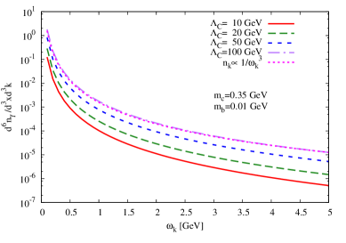
Figure 13: Photon spectra for an instantaneous mass shift for different values of $\Lambda_{C}$. In each case, they decay as $1/\omega^{3}_{\vec{k}}$ in the ultraviolet domain.

Furthermore, we investigate the dependence of the photon yield on the values of the constituent mass, $m_{c}$, and the bare mass, $m_{b}$, which is depicted in Fig. 14.

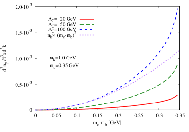
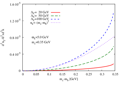
Figure 14: Dependence of the photon yield on the magnitude of the instantaneous mass shift for $\omega_{\vec{k}}=1.0\;\mathrm{GeV}$ (left panel) and $\omega_{\vec{k}}=5.0\;\mathrm{GeV}$ (right panel). For small mass shifts, the yield scales $\propto(m_{c}-m_{b})^{2}$, which is particularly visible for large values of $\Lambda_{C}$.

For small mass shifts, the photon yield scales with $(m_{c}-m_{b})^{2}$, which is particularly visible for large $\Lambda_{C}$. This can be understood by taking into account that the dominant contributions to (123) are given by (126b) and (127c), which for large $p$ both scale with occupation numbers $\propto(m_{c}-m_{b})^{2}/p^{2}$. For large mass shifts, i.e., for $m_{b}\rightarrow 0$ at fixed $m_{c}$, the photon yield starts to deviate from this quadratic scaling. In that limit, the photon yield diverges due to a collinear and an anti-collinear singularity in the loop integral. This issue will also be discussed in greater detail in appendix F. From the phenomenological point of view, however, it is not a serious problem since the quark masses stay finite even in the chirally restored phase.

IV.1.3 Summary of results

So far our investigations on chiral photon production have shown that the scenario of an instantaneous mass shift essentially comes along with three unphysical artifacts.

Firstly, the loop integral entering (62) features a linear divergence. In particular, this divergence arises from the contributions describing quark and antiquark bremsstrahlung and the interference between these two processes. It is caused by the quark and antiquark occupation numbers scaling $\propto(m_{c}-m_{b})^{2}/2p^{2}$ for $p\gg m_{b},m_{c}$. The latter is an artifact of the instantaneous change of the quark mass, and the mentioned divergence has been regulated by a cutoff at $p=\Lambda_{C}$.

Furthermore, we have seen that then the asymptotic photon spectra decay as $1/\omega^{3}_{\vec{k}}$ for any fixed value of $\Lambda_{C}$, which means that the total number density and the total energy density of the produced photons are logarithmically and linearly divergent, respectively.

Finally, the asymptotic photon yield diverges for $m_{b}\rightarrow 0$. We have demonstrated that this divergence is due to a collinear and an anticollinear singularity in the loop integral over the contributions (126b) and (126c) describing quark and antiquark bremsstrahlung and quark-antiquark annihilation into a photon, respectively. This is, however, a less serious problem than the two previous ones as it can be circumvented by leaving the bare mass, $m_{b}$, finite. The latter is justified from the phenomenological point of view since the quarks masses stay finite even in the chirally restored phase.

Hence, as the next step, we have to determine if and to which extent these problems are regulated if the chiral mass shift is assumed to take place over a finite time interval, $\tau$, which corresponds to a physically more realistic scenario.

IV.2 Mass shift over a finite time interval

IV.2.1 Calculation of photon numbers

For the general case of a mass shift over a finite time interval, $\tau$, both the time evolution of the fermionic wavefunctions, $\psi_{\vec{p},s,\uparrow\downarrow}(x)$, and the time integrals entering (59) require a numerical treatment. Hence, we have to find a way to extract the physical photon numbers from (59), i.e., the contributions which persist after taking the successive limits $t\rightarrow\infty$ and $\varepsilon\rightarrow 0$. For this purpose, we consider the photon self-energy in terms of positive- and negative-energy wavefunctions again,

$$\begin{split}\text{i}\Pi^{<}_{\mu\nu}(\vec{k},t_{1},t_{2})&=e^{2}\sum_{r,s}\int\frac{\text{d}^{3}p}{(2\pi)^{3}}\left[\bar{\psi}^{{}^{\prime}}_{\vec{p},r,\uparrow}(t_{1})\gamma_{\mu}\psi^{{}^{\prime}}_{\vec{p}+\vec{k},s,\downarrow}(t_{1})\right]\cdot\left[\bar{\psi}^{{}^{\prime}}_{\vec{p}+\vec{k},s,\downarrow}(t_{2})\gamma_{\nu}\psi^{{}^{\prime}}_{\vec{p},r,\uparrow}(t_{2})\right]\\ &=\sum_{r,s}\int\frac{d^{3}p}{(2\pi)^{3}}j_{\mu}(\vec{p},\vec{k},t_{1})j^{*}_{\nu}(\vec{p},\vec{k},t_{2})\ ,\end{split}$$ (130)

where we have introduced the effective current

$$j_{\mu}(\vec{p},\vec{k},r,s,t)=e\bar{\psi}^{{}^{\prime}}_{\vec{p},r,\uparrow}(t)\gamma_{\mu}\psi^{{}^{\prime}}_{\vec{p}+\vec{k},s,\downarrow}(t)\ .$$ (131)

Next, we rewrite

$$j_{\mu}(\vec{p},\vec{k},r,s,t) =e\left[\bar{\psi}^{{}^{\prime}}_{\vec{p},r,\uparrow}(t)\gamma_{\mu}\psi^{{}^{\prime}}_{\vec{p}+\vec{k},s,\downarrow}(t)-\bar{\psi}^{c,^{\prime}}_{\vec{p},r,\uparrow}(t)\gamma_{\mu}\psi^{c,^{\prime}}_{\vec{p}+\vec{k},s,\downarrow}(t)\right]+e\bar{\psi}^{c,^{\prime}}_{\vec{p},r,\uparrow}(t)\gamma_{\mu}\psi^{c,^{\prime}}_{\vec{p}+\vec{k},s,\downarrow}(t)$$

$$=j^{\text{MST}}_{\mu}(\vec{p},\vec{k},r,s,t)+j^{0}_{\mu}(\vec{p},\vec{k},r,s,t)\ ,$$ (132)

In analogy to $\psi^{{}^{\prime}}_{\vec{p},r,\uparrow\downarrow}(t)$, the expressions $\psi^{c,^{\prime}}_{\vec{p},r,\uparrow\downarrow}(t)$ are defined according to the relation

$$\psi^{c}_{\vec{p},r,\uparrow\downarrow}(x)=\psi^{c,^{\prime}}_{\vec{p},r,\uparrow\downarrow}(t)\text{e}^{\text{i}\vec{p}\cdot\vec{x}}\ .$$

Moreover, we have introduced

$$j^{\text{MST}}_{\mu}(\vec{p},\vec{k},r,s,t) = e\left[\bar{\psi}^{{}^{\prime}}_{\vec{p},r,\uparrow}(t)\gamma_{\mu}\psi^{{}^{\prime}}_{\vec{p}+\vec{k},s,\downarrow}(t)-\bar{\psi}^{c,^{\prime}}_{\vec{p},r,\uparrow}(t)\gamma_{\mu}\psi^{c,^{\prime}}_{\vec{p}+\vec{k},s,\downarrow}(t)\right]\ ,$$ (133a)

$$j^{0}_{\mu}(\vec{p},\vec{k},r,s,t) = e\bar{\psi}^{c,^{\prime}}_{\vec{p},r,\uparrow}(t)\gamma_{\mu}\psi^{c,^{\prime}}_{\vec{p}+\vec{k},s,\downarrow}(t)\ ,$$ (133b)

in the second step. Eq. (133a) vanishes if the quark mass is kept at its initial constituent value, $m_{c}$, for all times, $t$, but (133b) does not. As a consequence, these expressions can be considered as mass-shift (MST) and vacuum contribution to (131). With the help of (133), we can decompose the photon self-energy according to

$$\text{i}\Pi^{<}_{\mu\nu}(\vec{k},t_{1},t_{2})=\text{i}\Pi^{<,0}_{\mu\nu}(\vec{k},t_{1},t_{2})+\text{i}\Pi^{<,\text{MST}}_{\mu\nu}(\vec{k},t_{1},t_{2})+\text{i}\Pi^{<,\text{INT}}_{\mu\nu}(\vec{k},t_{1},t_{2})\ ,$$ (134)

with the individual contributions given by

$$\text{i}\Pi^{<,0}_{\mu\nu}(\vec{k},t_{1},t_{2})=\sum_{r,s}\int\frac{\text{d}^{3}p}{(2\pi)^{3}} j^{0}_{\mu}(\vec{p},\vec{k},r,s,t_{1})j^{0,*}_{\nu}(\vec{p},\vec{k},r,s,t_{2})\ ,$$ (135a)

$$\text{i}\Pi^{<,\text{MST}}_{\mu\nu}(\vec{k},t_{1},t_{2})=\sum_{r,s}\int\frac{\text{d}^{3}p}{(2\pi)^{3}} j^{\text{MST}}_{\mu}(\vec{p},\vec{k},r,s,t_{1})j^{\text{MST},*}_{\nu}(\vec{p},\vec{k},r,s,t_{2})\ ,$$ (135b)

$$\text{i}\Pi^{<,\text{INT}}_{\mu\nu}(\vec{k},t_{1},t_{2})=\sum_{r,s}\int\frac{\text{d}^{3}p}{(2\pi)^{3}} \left[j^{\text{MST}}_{\mu}(\vec{p},\vec{k},r,s,t_{1})j^{0,*}_{\nu}(\vec{p},\vec{k},r,s,t_{2})\right.$$

$$\left.+j^{0}_{\mu}(\vec{p},\vec{k},r,s,t_{1})j^{\text{MST},*}_{\nu}(\vec{p},\vec{k},r,s,t_{2})\right]\ .$$ (135c)

Expressions (135a) and (135b) describe the contributions from the vacuum polarization (VAC) and the mass shift (MST) to the overall photon self-energy, respectively, whereas (135c) characterizes their interference among each other (INT) . Hence, it is convenient to split up (59) accordingly

$$2\omega_{\vec{k}}\frac{\text{d}^{6}n^{\varepsilon}_{\gamma}(t)}{\text{d}^{3}x\text{d}^{3}k}=\left.2\omega_{\vec{k}}\frac{\text{d}^{6}n^{\varepsilon}_{\gamma}(t)}{\text{d}^{3}x\text{d}^{3}k}\right|_{\text{VAC}}+\left.2\omega_{\vec{k}}\frac{\text{d}^{6}n^{\varepsilon}_{\gamma}(t)}{\text{d}^{3}x\text{d}^{3}k}\right|_{\text{MST}}+\left.2\omega_{\vec{k}}\frac{\text{d}^{6}n^{\varepsilon}_{\gamma}(t)}{\text{d}^{3}x\text{d}^{3}k}\right|_{\text{INT}}\ .\\$$ (136)

The individual contributions read

$$\left.2\omega_{\vec{k}}\frac{\text{d}^{6}n^{\varepsilon}_{\gamma}(t)}{\text{d}^{3}x\text{d}^{3}k}\right|_{\text{VAC}} = \frac{\gamma^{\mu\nu}(k)}{(2\pi)^{3}}\int_{-\infty}^{t}dt_{1}\int_{-\infty}^{t}dt_{2}\mbox{ }\text{i}\Pi^{<,0}_{\nu\mu}(\vec{k},t_{1},t_{2})\text{e}^{\text{i}\omega_{\vec{k}}(t_{1}-t_{2})}\ ,$$ (137a)

$$\left.2\omega_{\vec{k}}\frac{\text{d}^{6}n^{\varepsilon}_{\gamma}(t)}{\text{d}^{3}x\text{d}^{3}k}\right|_{\text{MST}} = \frac{\gamma^{\mu\nu}(k)}{(2\pi)^{3}}\int_{-\infty}^{t}dt_{1}\int_{-\infty}^{t}dt_{2}\mbox{ }\text{i}\Pi^{<,\text{MST}}_{\nu\mu}(\vec{k},t_{1},t_{2})\text{e}^{\text{i}\omega_{\vec{k}}(t_{1}-t_{2})}\ ,$$ (137b)

$$\left.2\omega_{\vec{k}}\frac{\text{d}^{6}n^{\varepsilon}_{\gamma}(t)}{\text{d}^{3}x\text{d}^{3}k}\right|_{\text{INT}} = \frac{\gamma^{\mu\nu}(k)}{(2\pi)^{3}}\int_{-\infty}^{t}dt_{1}\int_{-\infty}^{t}dt_{2}\mbox{ }\text{i}\Pi^{<,\text{INT}}_{\nu\mu}(\vec{k},t_{1},t_{2})\text{e}^{\text{i}\omega_{\vec{k}}(t_{1}-t_{2})}\ .$$ (137c)

In appendix A it is shown that the contribution from the vacuum polarization (135a) vanishes under the successive limits $t\rightarrow\infty$ and then $\varepsilon\rightarrow 0$. We now demonstrate that the contribution from the interference term (135c) is also eliminated by this procedure so that only the mass-shift contribution (137b) remains and thus describes the physical photon number. For this purpose, we first rewrite the asymptotic contributions from (135b) and (135c) at finite $\varepsilon$ by interchanging the time integrals with the loop integral over $\text{d}^{3}p$. This leads to

$$\left.2\omega_{\vec{k}}\frac{\text{d}^{6}n^{\varepsilon}_{\gamma}}{\text{d}^{3}x\text{d}^{3}k}\right|_{\text{MST}}=\frac{\gamma^{\mu\nu}(k)}{(2\pi)^{3}}\sum_{r,s}\int\frac{\text{d}^{3}p}{(2\pi)^{3}} I^{\varepsilon,*}_{\mu}(\vec{p},\vec{k},r,s)I^{\varepsilon}_{\nu}(\vec{p},\vec{k},r,s)\ ,$$ (138a)

$$\left.2\omega_{\vec{k}}\frac{\text{d}^{6}n^{\varepsilon}_{\gamma}}{\text{d}^{3}x\text{d}^{3}k}\right|_{\text{INT}}=\frac{\gamma^{\mu\nu}(k)}{(2\pi)^{3}}\sum_{r,s}\int\frac{\text{d}^{3}p}{(2\pi)^{3}} \left[I^{\varepsilon,*}_{\mu}(\vec{p},\vec{k},r,s)J^{\varepsilon}_{\nu}(\vec{p},\vec{k},r,s)\right.$$

$$+\left.J^{\varepsilon,*}_{\mu}(\vec{p},\vec{k},r,s)I^{\varepsilon}_{\nu}(\vec{p},\vec{k},r,s)\right]\ .$$ (138b)

In order to keep the notation short, we have introduced

$$I^{\varepsilon}_{\mu}(\vec{p},\vec{k},r,s) = \int_{-\infty}^{\infty}\text{d}tf_{\varepsilon}(t)j^{\text{MST}}_{\mu}(\vec{p},\vec{k},r,s,t)\text{e}^{\text{i}\omega_{\vec{k}}t}\ ,$$ (139a)

$$J^{\varepsilon}_{\mu}(\vec{p},\vec{k},r,s) = \int_{-\infty}^{\infty}\text{d}tf_{\varepsilon}(t)j^{0}_{\mu}(\vec{p},\vec{k},r,s,t)\text{e}^{\text{i}\omega_{\vec{k}}t}\ ,$$ (139b)

The time integral in (139b) evaluates to

$$J^{\varepsilon}_{\mu}(\vec{p},\vec{k},r,s)=e\bar{u}_{c}(\vec{p},s)\gamma_{\mu}v_{c}(\vec{p}+\vec{k},s)\frac{2\varepsilon}{\varepsilon^{2}+\omega^{c,2}_{1}(\vec{p},\vec{k})}\ ,$$ (140)

with $\omega^{c}_{1}(\vec{p},\vec{k})$ given by (118a). To handle the time integral entering (139a), we first split

$$I^{\varepsilon}_{\mu}(\vec{p},\vec{k},r,s)=\int_{-\infty}^{T}\text{d}tf_{\varepsilon}(t)j^{\text{MST}}_{\mu}(\vec{p},\vec{k},r,s,t)\text{e}^{\text{i}\omega_{\vec{k}}t}+\int_{T}^{\infty}\text{d}tf_{\varepsilon}(t)j^{\text{MST}}_{\mu}(\vec{p},\vec{k},r,s,t)\text{e}^{\text{i}\omega_{\vec{k}}t}\ ,$$ (141)

where $T\gg\tau$. Next we take into account that for $t\geq T$, the fermionic wavefunctions have essentially turned into superpositions of positive- and negative-energy states with respect to the final bare mass, $m_{b}$, i.e.,

$$\psi^{{}^{\prime}}_{\vec{p},s,\uparrow}(t) = \tilde{\alpha}_{\vec{p}}\psi^{b,^{\prime}}_{\vec{p},s,\uparrow}(t)+\tilde{\beta}_{\vec{p}}\psi^{b,^{\prime}}_{\vec{p},s,\downarrow}(t)\ ,$$ (142a)

$$\psi^{{}^{\prime}}_{\vec{p},s,\downarrow}(t) = \tilde{\gamma}_{\vec{p}}\psi^{b,^{\prime}}_{\vec{p},s,\downarrow}(t)+\tilde{\delta}_{\vec{p}}\psi^{b,^{\prime}}_{\vec{p},s,\uparrow}(t)\ ,$$ (142b)

with the coefficients not depending on time. We have introduced the $\tilde{\cdot}$ notation in order to highlight that the expansion coefficients are generally different from those for an instantaneous mass shift given by (95a). With the help of (142), expression (141) is further evaluated to

$$\begin{split}I^{\varepsilon}_{\mu}(\vec{p},\vec{k},r,s)=&\int_{-\infty}^{T}\text{d}tf_{\varepsilon}(t)j^{\text{MST}}_{\mu}(\vec{p},\vec{k},r,s,t)\text{e}^{\text{i}\omega_{\vec{k}}t}\\ +&e\left\{\tilde{\alpha}^{*}_{\vec{p}}\tilde{\gamma}_{\vec{p}+\vec{k}}\bar{u}_{b}(\vec{p},r)\gamma_{\mu}v_{b}(\vec{p}+\vec{k},s)\frac{\text{e}^{-\left[\varepsilon-\text{i}\omega^{b}_{1}(\vec{p},\vec{k})\right]T}}{\varepsilon-\text{i}\omega^{b}_{1}(\vec{p},\vec{k})}\right.\\ &+\tilde{\alpha}^{*}_{\vec{p}}\tilde{\delta}_{\vec{p}+\vec{k}}\bar{u}_{b}(\vec{p},r)\gamma_{\mu}u_{b}(\vec{p}+\vec{k},s)\frac{\text{e}^{-\left[\varepsilon+\text{i}\omega^{b}_{2}(\vec{p},\vec{k})\right]T}}{\varepsilon+\text{i}\omega^{b}_{2}(\vec{p},\vec{k})}\\ &+\tilde{\beta}^{*}_{\vec{p}}\tilde{\gamma}_{\vec{p}+\vec{k}}\bar{v}_{b}(\vec{p},r)\gamma_{\mu}v_{b}(\vec{p}+\vec{k},s)\frac{\text{e}^{-\left[\varepsilon-\text{i}\omega^{b}_{3}(\vec{p},\vec{k})\right]T}}{\varepsilon-\text{i}\omega^{b}_{3}(\vec{p},\vec{k})}\\ &+\tilde{\beta}^{*}_{\vec{p}}\tilde{\delta}_{\vec{p}+\vec{k}}\bar{v}_{b}(\vec{p},r)\gamma_{\mu}u_{b}(\vec{p}+\vec{k},s)\frac{\text{e}^{-\left[\varepsilon+\text{i}\omega^{b}_{4}(\vec{p},\vec{k})\right]T}}{\varepsilon+\text{i}\omega^{b}_{4}(\vec{p},\vec{k})}\\ &-\left.\bar{u}_{c}(\vec{p},r)\gamma_{\mu}v_{c}(\vec{p}+\vec{k},s)\frac{\text{e}^{-\left[\varepsilon-\text{i}\omega^{c}_{1}(\vec{p},\vec{k})\right]T}}{\varepsilon-\text{i}\omega^{c}_{1}(\vec{p},\vec{k})}\right\}\ .\end{split}$$ (143)

Since the frequencies (118a)-(118d) are either positive or negative definite, taking the limit $\varepsilon\rightarrow 0$ leads to

$$\begin{split}I^{\varepsilon}_{\mu}(\vec{p},\vec{k},r,s)\rightarrow I_{\mu}(\vec{p},\vec{k},r,s)=&\int_{-\infty}^{T}\text{d}t\mbox{ }j^{\text{MST}}_{\mu}(\vec{p},\vec{k},r,s,t)\text{e}^{\text{i}\omega_{\vec{k}}t}\\ +&\text{i}e\left[\tilde{\alpha}^{*}_{\vec{p}}\tilde{\gamma}_{\vec{p}+\vec{k}}\bar{u}_{b}(\vec{p},r)\gamma_{\mu}v_{b}(\vec{p}+\vec{k},s)\frac{\text{e}^{\text{i}\omega^{b}_{1}(\vec{p},\vec{k})}}{\omega^{b}_{1}(\vec{p},\vec{k})}\right.\\ &-\tilde{\alpha}^{*}_{\vec{p}}\tilde{\delta}_{\vec{p}+\vec{k}}\bar{u}_{b}(\vec{p},r)\gamma_{\mu}u_{b}(\vec{p}+\vec{k},s)\frac{\text{e}^{-\text{i}\omega^{b}_{2}(\vec{p},\vec{k})}}{\omega^{b}_{2}(\vec{p},\vec{k})}\\ &+\tilde{\beta}^{*}_{\vec{p}}\tilde{\gamma}_{\vec{p}+\vec{k}}\bar{v}_{b}(\vec{p},r)\gamma_{\mu}v_{b}(\vec{p}+\vec{k},s)\frac{\text{e}^{\text{i}\omega^{b}_{3}(\vec{p},\vec{k})}}{\omega^{b}_{3}(\vec{p},\vec{k})}\\ &-\tilde{\beta}^{*}_{\vec{p}}\tilde{\delta}_{\vec{p}+\vec{k}}\bar{v}_{b}(\vec{p},r)\gamma_{\mu}u_{b}(\vec{p}+\vec{k},s)\frac{\text{e}^{-\text{i}\omega^{b}_{4}(\vec{p},\vec{k})}}{\omega^{b}_{4}(\vec{p},\vec{k})}\\ &-\left.\bar{u}_{c}(\vec{p},r)\gamma_{\mu}v_{c}(\vec{p}+\vec{k},s)\frac{\text{e}^{\text{i}\omega^{c}_{1}(\vec{p},\vec{k})}}{\omega^{c}_{1}(\vec{p},\vec{k})}\right]\ .\end{split}$$ (144)

We are allowed to interchange the limiting process with the remaining time integral since $j^{\text{MST}}_{\mu}(\vec{p},\vec{k},r,s,t)\text{e}^{\text{i}\omega_{\vec{k}}t}$ vanishes for $t\rightarrow-\infty$ and is thus integrable by itself on the time interval $(-\infty;T]$. As we also have from (140)

$$J^{\varepsilon}_{\mu}(\vec{p},\vec{k},r,s)=e\bar{u}_{c}(\vec{p},r)\gamma_{\mu}v_{c}(\vec{p}+\vec{k},s)\frac{2\varepsilon}{\omega^{c,2}_{1}(\vec{p},\vec{k})}+\mathcal{O}(\varepsilon^{2})\ ,\ \mbox{for}\ \varepsilon\rightarrow 0\ ,$$ (145)

the interference contribution vanishes in that limit. Furthermore, the mass-shift contribution, which as a consequence of the above describes the actual photon number, turns into

$$2\omega_{\vec{k}}\frac{\text{d}^{6}n_{\gamma}}{\text{d}^{3}x\text{d}^{3}k}=\frac{\gamma^{\mu\nu}(k)}{(2\pi)^{3}}\sum_{r,s}\int\frac{\text{d}^{3}p}{(2\pi)^{3}}I^{*}_{\mu}(\vec{p},\vec{k},r,s)I_{\nu}(\vec{p},\vec{k},r,s)\ .$$ (146)

It follows from (146) and (144) that solving the equations of motion (36) numerically on the time interval $[-T;T]$ essentially provides all the information required to evaluate $I_{\mu}(\vec{p},\vec{k},r,s)$ and the asymptotic photon numbers (146). We have $j^{\text{MST}}_{\mu}(\vec{p},\vec{k},r,s,t)\approx 0$ for $t\leq-T$ since $T\gg\tau$. We thus can approximate

$$\int_{-\infty}^{T}\text{d}t\mbox{ }j^{\text{MST}}_{\mu}(\vec{p},\vec{k},r,s,t)\text{e}^{\text{i}\omega_{\vec{k}}t}\approx\int_{-T}^{T}\text{d}t\mbox{ }j^{\text{MST}}_{\mu}(\vec{p},\vec{k},r,s,t)\text{e}^{\text{i}\omega_{\vec{k}}t}\ .$$

Hence, the numerical solution of (36) on $[-T;T]$ allows us to evaluate the time integral entering (146) with sufficiently high accuracy. Based on this solution, the asymptotic expansion coefficients can be projected out from (142) at $t=T$.

So far, we have restricted ourselves to the scenario where the quark mass is only changed from its constituent value, $m_{c}$, to its bare value, $m_{b}$. When considering the second scenario, where the quark mass is first changed from $m_{c}$ to $m_{b}$ and then back to $m_{c}$, the asymptotic photon number is, however, determined mostly in the same way. The only difference is that $T$ then has to be chosen such that $T\gg\tau+\frac{\tau_{L}}{2}$ with $\tau_{L}$ denoting the lifetime of the chirally restored phase. Moreover, one has to take into account that the fermionic wavefunctions have turned into superpositions of positive- and negative-energy states of mass $m_{c}$ instead of mass $m_{b}$ for $t\geq T$, i.e.,

$$\psi^{{}^{\prime}}_{\vec{p},s,\uparrow}(t) = \tilde{\alpha}_{\vec{p}}\psi^{c,^{\prime}}_{\vec{p},s,\uparrow}(t)+\tilde{\beta}_{\vec{p}}\psi^{c,^{\prime}}_{\vec{p},s,\downarrow}(t)\ ,$$ (147a)

$$\psi^{{}^{\prime}}_{\vec{p},s,\downarrow}(t) = \tilde{\gamma}_{\vec{p}}\psi^{c,^{\prime}}_{\vec{p},s,\downarrow}(t)+\tilde{\delta}_{\vec{p}}\psi^{c,^{\prime}}_{\vec{p},s,\uparrow}(t)\ .$$ (147b)

Accordingly, expression (144) is replaced by

$$\begin{split}I_{\mu}(\vec{p},\vec{k},r,s)=&\int_{-\infty}^{T}\text{d}t\mbox{ }j^{\text{MST}}_{\mu}(\vec{p},\vec{k},r,s,t)\text{e}^{\text{i}\omega_{\vec{k}}t}\\ +&\text{i}e\left[\left(\tilde{\alpha}^{*}_{\vec{p}}\tilde{\gamma}_{\vec{p}+\vec{k}}-1\right)\bar{u}_{c}(\vec{p},r)\gamma_{\mu}v_{c}(\vec{p}+\vec{k},s)\frac{\text{e}^{\text{i}\omega^{c}_{1}(\vec{p},\vec{k})}}{\omega^{c}_{1}(\vec{p},\vec{k})}\right.\\ &-\tilde{\alpha}^{*}_{\vec{p}}\tilde{\delta}_{\vec{p}+\vec{k}}\bar{u}_{c}(\vec{p},r)\gamma_{\mu}u_{c}(\vec{p}+\vec{k},s)\frac{\text{e}^{-\text{i}\omega^{c}_{2}(\vec{p},\vec{k})}}{\omega^{c}_{2}(\vec{p},\vec{k})}\\ &+\tilde{\beta}^{*}_{\vec{p}}\tilde{\gamma}_{\vec{p}+\vec{k}}\bar{v}_{c}(\vec{p},r)\gamma_{\mu}v_{c}(\vec{p}+\vec{k},s)\frac{\text{e}^{\text{i}\omega^{c}_{3}(\vec{p},\vec{k})}}{\omega^{c}_{3}(\vec{p},\vec{k})}\\ &\left.-\tilde{\beta}^{*}_{\vec{p}}\tilde{\delta}_{\vec{p}+\vec{k}}\bar{v}_{c}(\vec{p},r)\gamma_{\mu}u_{c}(\vec{p}+\vec{k},s)\frac{\text{e}^{-\text{i}\omega^{c}_{4}(\vec{p},\vec{k})}}{\omega^{c}_{4}(\vec{p},\vec{k})}\right]\ .\end{split}$$ (148)

For completeness, we mention that with the help of

$$\gamma^{\mu\nu}(k)=\sum_{\lambda}\varepsilon^{\mu,*}(\vec{k},\lambda)\varepsilon^{\nu}(\vec{k},\lambda)\ ,$$

expression (146) can be brought into the following alternative absolute-square representation

$$2\omega_{\vec{k}}\frac{\text{d}^{6}n_{\gamma}}{\text{d}^{3}x\text{d}^{3}k}=\frac{1}{(2\pi)^{3}}\sum_{\lambda,r,s}\int\frac{\text{d}^{3}p}{(2\pi)^{3}}\left|\varepsilon^{\mu}(\vec{k},\lambda)I_{\mu}(\vec{p},\vec{k},r,s)\right|^{2}\ .$$ (149)

Thus, the photon number is positive (semi-) definite and cannot acquire unphysical negative values. Furthermore, it vanishes if no mass shift takes place at all since we then have $j^{\text{MST}}_{\mu}(\vec{p},\vec{k},r,s,t)\equiv 0$.

IV.2.2 Numerical investigations and results

First of all, we have to determine whether the linear divergence in the loop integral entering expression (62) for the photon yield is cured if the mass shift is assumed to take place over a finite time interval, $\tau$. For this purpose, we consider the cutoff dependence of the asymptotic photon number for different photon energies, $\omega_{\vec{k}}$, and different mass parameterizations, $m_{i}(t)$, which is depicted in Fig. 15. As mass parameters, we have again chosen $m_{c}=0.35\;\mathrm{GeV}$ and $m_{b}=0.01\;\mathrm{GeV}$.

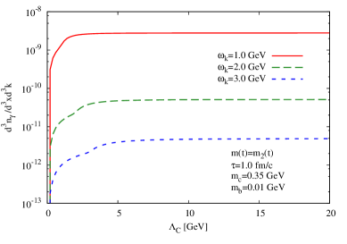
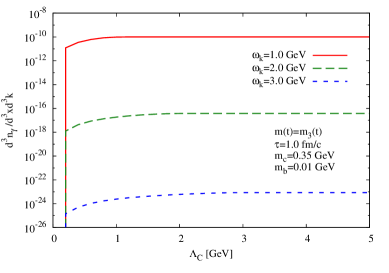
Figure 15: Cutoff dependence of asymptotic photon numbers for $m_{2}(t)$ (left panel) and $m_{3}(t)$ (right panel). In both cases, we have chosen $\tau=1.0\;\mathrm{fm}/c$. The parameterizations $m_{i}(t)$ are shown in Fig. 2 and defined in (92). The loop integral is rendered finite and its saturation behavior crucially depends on the order of differentiability of the considered mass parametrization.

We see that the linear divergence, which has shown up in the loop integral for an instantaneous mass shift, is absent for both parameterizations $m_{2}(t)$ and $m_{3}(t)$. In particular, the order of differentiability of the considered mass parametrization, $m_{i}(t)$, is crucial for the saturation behavior of the loop integral. For $m_{2}(t)$ being continuously differentiable once, the loop integral saturates at $\Lambda_{C}\simeq 10\;\mathrm{GeV}$ whereas it exhibits a much faster saturation already at $\Lambda_{C}\simeq 2.0-3.0\;\mathrm{GeV}$ for $m_{3}(t)$ being continuously differentiable infinitely many times. Since the latter parametrization describes the most physical scenario, chiral photon production can be considered as a low-momentum phenomenon.

As the loop integral is finite for a mass shift over a finite time interval, $\tau$, we can now turn to the UV behavior of the resulting photon spectra. Fig. 16 compares the resulting photon spectra for the different mass parameterizations. For $m_{2}(t)$ and $m_{3}(t)$, a transition time of $\tau=1.0\;\mathrm{fm}/c$ has been assumed.

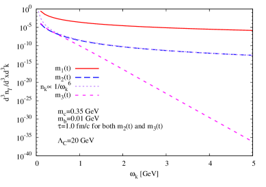
Figure 16: Asymptotic photon spectra for the different mass parameterizations given by Eqs. (92). If one turns from an instantaneous mass shift ($m_{1}(t)$) to a mass shift over a finite time interval ($m_{2,3}(t)$), the photon spectra are rendered integrable in the ultraviolet domain. Furthermore, their decay behavior there is highly sensitive to the order of differentiability of the considered mass parametrization, $m_{i}(t)$.

Analogously to the particle spectra investigated in section III, we see that the asymptotic photon spectra exhibit a strong sensitivity to the order of differentiability, i.e., the ‘smoothness’ of the considered mass parametrization, $m_{i}(t)$. In particular, the decay behavior in the ultraviolet domain is suppressed from $\propto 1/\omega^{3}_{\vec{k}}$ to $\propto 1/\omega^{6}_{\vec{k}}$ if we turn from $m_{1}(t)$ (discontinuous parametrization) to $m_{2}(t)$ (parametrization being continuously differentiable once). The logarithmic and linear UV divergences in the total photon-number density and the total energy density, respectively, are thus cured. Furthermore, if we consider the photon spectra for $m_{3}(t)$, which is continuously differentiable infinitely many times and hence describes the most physical scenario, the photon numbers in the UV domain are suppressed even further to an exponential decay.

As one can infer from Fig. 17, the decay behavior of the photon spectra is highly sensitive to the considered transition time, $\tau$, for both $m_{2}(t)$ and $m_{3}(t)$. In each case, the suppression of the photon numbers compared to the instantaneous case is the stronger the more slowly the mass shift is assumed to take place. As expected, both parameterizations reproduce the photon spectra for an instantaneous mass shift in the limit $\tau\rightarrow 0$.

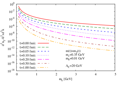
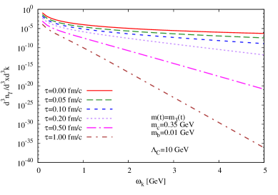
Figure 17: Asymptotic photon spectra for different transition times, $\tau$, for $m_{2}(t)$ (left panel) and $m_{3}(t)$ (right panel). The suppression of the photon numbers with respect to the instantaneous case is the stronger the more slowly ($\tau$ increasing) the mass shift is assumed to take place.

It should be mentioned that because of finite machine precision, it was first difficult to resolve the photon numbers numerically for $m_{3}(t)$ and $\tau=1.0$ fm/c in the domain $\omega_{\vec{k}}\geq 2.5$ GeV. For that reason, the photon numbers in that domain have been extrapolated from those for $1.5\leq\omega_{\vec{k}}\leq 2.5$ GeV by performing a linear regression of the logarithms of the photon numbers.

We shall briefly point out why we have to go to comparatively small transition times of $\tau\simeq 0.02\;\mathrm{fm}/c$ for the photon numbers to be again of the same order of magnitude as for an instantaneous mass shift. The main reason is the different convergence behavior of the loop integral for different mass parameterizations. For the case of an instantaneous mass shift it features a linear divergence, which means that all momentum modes with $p\gg m_{c},m_{b}$ and $p\gg\omega_{\vec{k}}$ contribute more or less equally to (62). For the case of a mass shift over a finite time interval, $\tau$, however, the loop integral is UV finite so that the contributions from the different momentum modes are suppressed with increasing $p$. This implies that the suppression of (62) for given $\tau$ with respect to the instantaneous case, $m_{1}(t)$, is the stronger the larger the value of $\Lambda_{C}$ is chosen. Therefore, the larger $\Lambda_{C}$ is chosen the smaller $\tau$ has to be taken in order to approximately reproduce the photon yield for $m_{1}(t)$. This can also be inferred from Fig. 18 displaying the cutoff dependence of the photon yield for $\omega_{\vec{k}}=1.0\;\mathrm{GeV}$ and different transition times, $\tau$.

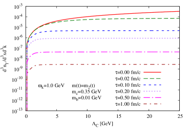
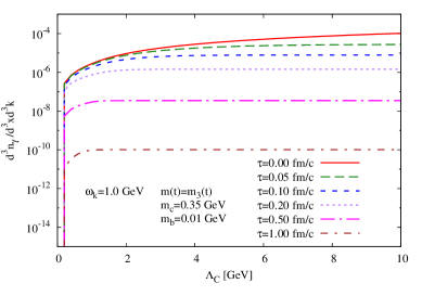
Figure 18: Cutoff dependence of the photon yield for $m_{2}(t)$ (left panel) and $m_{3}(t)$ (right panel) at different values of $\tau$. For given finite $\tau$ the suppression compared to the instantaneous case is the stronger the larger $\Lambda_{C}$ is chosen.

For completeness, we also investigate the dependence of the resulting photon spectra on the magnitude of the mass shift, which is depicted in Fig. 19.

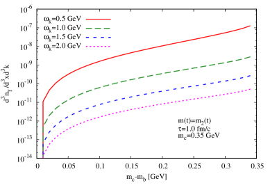
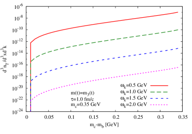
Figure 19: Dependence of the photon numbers on the considered bare mass, $m_{b}$, for $m_{2}(t)$ (left panel) and $m_{3}(t)$ (right panel). As in the instantaneous case, the photon numbers increase with the magnitude of the mass shift and the behavior in the limit $m_{b}\rightarrow 0$ indicates a divergence therein.

Similarly to the instantaneous case, the photon yield arising from the chiral mass shift increases with the magnitude of the latter. The change in curvature which appears for $m_{b}\rightarrow 0$ indicates a possible divergence in this limit which, in analogy to the instantaneous case, could arise from a collinear and/or anticollinear singularity in the loop integral entering (62). This still requires further investigation.

As for the asymptotic quark/antiquark occupation numbers, we also consider the scenario where the fermion mass is first changed from $m_{c}$ to $m_{b}$ and then back to $m_{c}$ to take into account the finite lifetime of the chirally restored phase. Fig. 20 shows the photon spectra for different values of $\Lambda_{C}$ for both mass shifts taking place instantaneously which is described by $\tilde{m}_{1}(t)$. We have assumed a lifetime of $\tau_{L}=4.0$ fm/c for the chirally restored phase.

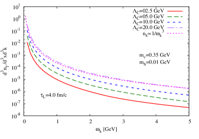
Figure 20: Asymptotic photon spectra for both mass shifts taking place instantaneously. The loop integral in (62) is again linearly divergent. Furthermore, the photon spectra decay as $1/\omega_{\vec{k}}^{3}$ if this divergence is regulated via a cutoff at $p=\Lambda_{C}$.

As for the first scenario, the loop integral entering (62) exhibits a linear divergence. If this divergence is regulated via a cutoff at $p=\Lambda_{C}$, the resulting photon spectrum again decays $\propto 1/\omega^{3}_{\vec{k}}$ in the ultraviolet domain and is hence not integrable. As one would expect from the first scenario, however, these pathologies are again artifacts from the (unphysical) instantaneous mass shifts and are resolved if both mass shifts are assumed to take place over a finite time interval, $\tau$.

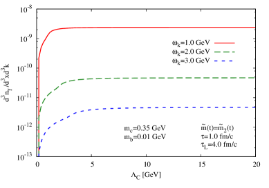
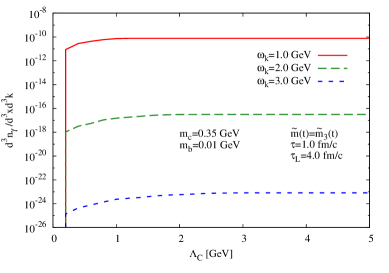
Figure 21: Cutoff dependence of asymptotic photon numbers for $\tilde{m}_{2}(t)$ (left panel) and $\tilde{m}_{3}(t)$ (right panel). In both cases, we have chosen $\tau=1.0\;\mathrm{fm}/c$ and $\tau_{L}=4.0\;\mathrm{fm}/c$. The parameterizations $\tilde{m}_{i}(t)$ are shown in Fig. 8 and defined in (105). Like in the first scenario, the loop integral is rendered finite and its saturation behavior crucially depends on the order of differentiability of the considered mass parametrization.

In particular, one can infer from Fig. 21 that the loop integral again saturates around $\Lambda_{C}=10\;\mathrm{GeV}$ and $\Lambda_{C}=2$-$3\;\mathrm{GeV}$ for $\tilde{m}_{2}(t)$ and $\tilde{m}_{3}(t)$, respectively. Moreover, Fig. 22 shows that the resulting photon spectra exhibit the same sensitivity to the order of differentiability of the considered mass parametrization, $\tilde{m}_{i}(t)$, just like in the previous case. The photon spectra decay $\propto 1/\omega^{6}_{\vec{k}}$ for $\tilde{m}_{2}(t)$ (continuously differentiable once) in the ultraviolet domain and are suppressed further to an exponential decay for $\tilde{m}_{3}(t)$ (continuously differentiable infinitely many times).

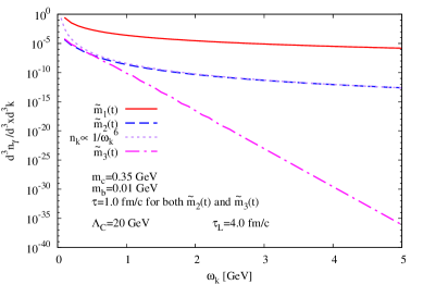
Figure 22: Asymptotic photon spectra for the different mass parameterizations given by Eqs. (105). As expected, the photon spectra are again rendered integrable in the ultraviolet domain if both mass changes take place over a finite time interval, $\tau$. Furthermore, they show the same sensitivity to the order of differentiability of the considered mass parametrization, $\tilde{m}_{i}(t)$, as for a single mass change.

As it must be, the photon spectra show the same sensitivity to the change duration, $\tau$, as for the first scenario, i.e., the suppression of the photon numbers compared to the instantaneous case is the stronger the more slowly that mass changes are assumed to take place. Moreover, both $\tilde{m}_{2}(t)$ and $\tilde{m}_{3}(t)$ reproduce the photon spectra for the instantaneous case in the limit $\tau\rightarrow 0$. This is shown in Fig. 23.

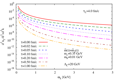
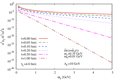
Figure 23: Asymptotic photon numbers for different transition times, $\tau$, for $\tilde{m}_{2}(t)$ (left panel) and $\tilde{m}_{3}(t)$ (right panel). As in the previous scenario, the suppression of the photon numbers with respect to the instantaneous case is the stronger the more slowly ($\tau$ increasing) the mass shifts are assumed to take place.

Hence, we have seen so far that the general dependence of the photon numbers in the ultraviolet domain on the order of differentiability of $\tilde{m}(t)$ and the transition time, $\tau$, is the same as for the first scenario, which one would also expect intuitively. Nevertheless, there are some differences in the dependence on the magnitude of the mass shift, $m_{c}-m_{b}$, which can be seen in Fig 24.

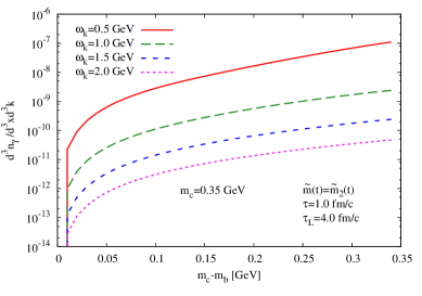
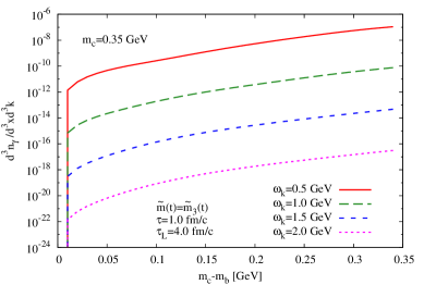
Figure 24: Dependence of the photon numbers on the considered bare mass, $m_{b}$, for $\tilde{m}_{2}(t)$ (left panel) and $\tilde{m}_{3}(t)$ (right panel). Like for the scenario where the mass is solely changed form $m_{c}$ to $m_{b}$, the photon numbers increase with the magnitude of the mass shift, $m_{c}-m_{b}$. Their behavior in the limit $m_{b}\rightarrow 0$ does, however, not indicate a divergence.

As in the previous case, the photon yield increases with the magnitude of the mass difference for given photon energy, $\omega_{\vec{k}}$. The crucial difference, however, is that the curvature does not change for $m_{b}\rightarrow 0$. This indicates that, in contrast to the first scenario, the photon numbers converge in that limit and that the loop integral entering (62) does not feature a collinear and/or an anticollinear divergence therein.

We have seen in section III that the asymptotic quark and antiquark occupation numbers for $p\gg m_{c},m_{b}$ are modified by a factor of $4\sin^{2}{p\tau_{L}}$ when turning from $m_{i}(t)$ to $\tilde{m}_{i}(t)$ ($i=1,2,3$) for any given transition time, $\tau$. In contrast, the asymptotic photon numbers in the ultraviolet domain do not exhibit a similar modification by a factor of $4\sin^{2}{\omega_{\vec{k}}\tau_{L}}$. Solely for $\tilde{m}_{3}(t)$ the photon spectra exhibit a slightly oscillating behavior (see e.g. right panel of Fig. 23) in the photon momentum, $k$, for sufficiently large values of $\tau$. For $m_{3}(t)$ and $\tau=1.0\;\mathrm{fm}/c$ this behavior can only be displayed up to $\omega_{\vec{k}}=2.5$ GeV since the photon numbers for $\omega_{\vec{k}}>2.5$ GeV have again been extrapolated from those for $1.5\leq\omega_{\vec{k}}\leq 2.5$ GeV by a linear regression.

Even though one might expect a similar modification as for the asymptotic quark/antiquark occupation numbers in the first place, there are two important aspects to be taken into account. On the one hand, the asymptotic photon numbers incorporate the entire history of the fermionic wavefunction and hence of the quark and antiquark occupation numbers, which are extracted from the former. In particular, the occupation numbers partially coincide with the asymptotic ones of the first scenario between the two mass shifts. On the other hand, it follows from (62) that the dependence of the wavefunction parameters on the fermion momenta is integrated out when determining the asymptotic photon numbers. Upon this procedure, a possible oscillating behavior in the individual contributions to (62) from the different momentum modes can get lost again.

The latter aspect is supported when comparing the asymptotic photon numbers for both parameterizations $m_{i}(t)$ and $\tilde{m}_{i}(t)$, which is done in Fig. 25 for fixed photon energies, $\omega_{\vec{k}}$, and different magnitudes of the mass shift, $m_{c}-m_{b}$.

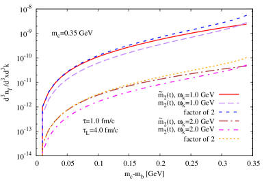
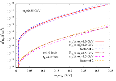
Figure 25: Comparison of photon numbers for $m_{2}(t)$ and $\tilde{m}_{2}(t)$ (left panel) and for $m_{3}(t)$ and $\tilde{m}_{3}(t)$ (right panel). For small mass shifts, $m_{c}-m_{b}$, the photon numbers differ by a factor of roughly $2$, which is particularly distinctive for $m_{2}(t)$ and $\tilde{m}_{2}(t)$, respectively.

There the dotted lines represent the photon spectra of $m_{i}(t)$ multiplied by a factor of $2$ in each case. Hence, for small magnitudes of $m_{c}-m_{b}$, the photon numbers roughly double if the quark/antiquark mass is switched back to its constituent value, $m_{c}$. The latter feature is particularly distinctive for $\tilde{m}_{2}(t)$. Such a result is understandable since both mass shifts are expected to give a comparable contribution to the asymptotic photon yield (62). But in particular, integrating out an additional factor of $4\sin^{2}{p\tau_{L}}$ gives rise to an overall rescaling by a factor of roughly $2$ if the integrand does not change significantly over the periodicity interval $\Delta p=\pi/\tau_{L}$. For increasing $m_{c}-m_{b}$, the asymptotic photon numbers for $m_{i}(t)$ and $\tilde{m}_{i}(t)$ start to deviate from this ratio as the different scaling behavior for $m_{b}\rightarrow 0$ starts to manifest itself.

In contrast to Wang and Boyanovsky (2001); Wang et al. (2002); Boyanovsky and de Vega (2003), our asymptotic photon numbers arising from first-order QED processes are UV finite for both scenarios if the mass shifts are assumed to take place over a finite time interval, $\tau$. Hence, it is convenient to compare them to leading-order thermal contributions. We note again that first-order QED contributions vanish in a static thermal equilibrium. There the first non-trivial contribution starts at two-loop order. Since a loop expansion does not coincide with a coupling-constant expansion, resummations are necessary to obtain the thermal rate at quartic order in the perturbative coupling constants, i.e. at linear order in $\alpha_{e}$ and at linear order in $\alpha_{s}$ Arnold et al. (2001a). Fig. 26 shows the photon numbers from first-order chiral photon production together with leading-order thermal contributions. The latter have been obtained by integrating the leading order thermal rates taken from Arnold et al. (2001a) over the lifetime interval of the chirally restored phase, $\tau_{L}=4.0$ fm/c, at a temperature of $T=0.2$ GeV.

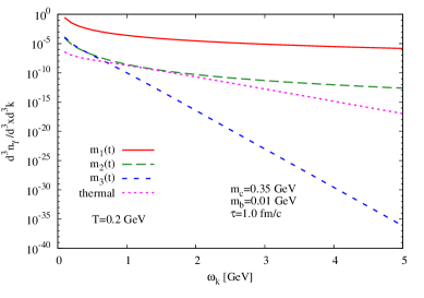
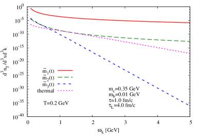
Figure 26: Comparison of first-order mass-shift contributions to time-integrated thermal rates for $m_{i}(t)$ (left panel) and $\tilde{m}_{i}(t)$ (right panel). For $i=3$ most likely characterizing a physical scenario, the photon spectra arising from the chiral mass shift are clearly subdominant for $\omega_{\vec{k}}\gtrsim 1.0$ GeV.

In this context, the photon spectra for $\tilde{m}_{i}(t)$ are the more meaningful ones, as the underlying scenario considers the finite lifetime of the chirally restored phase during a heavy-ion collision. Nevertheless, we see that for both $m_{3}(t)$ and $\tilde{m}_{3}(t)$, which are continuously differentiable infinitely many times and thus represent the most physical scenario, the photon numbers for $\omega_{\vec{k}}\gtrsim 1.0$ GeV are subdominant compared to those obtained from (time-integrated) thermal rates for phenomenologically reasonable choices of $\tau$ and $T$.

To summarize, we have seen that, if we turn from an instantaneous mass shift to a mass shift over a finite time interval, $\tau$, the linear divergence in the loop integral is regulated. Furthermore, the asymptotic photon spectra are integrable in the ultraviolet domain if the time evolution of the quark masses is described in a physical way. Finally, the decay behavior shows a strong sensitivity to the considered transition time, $\tau$, of the quark mass and we recover our results for an instantaneous mass shift as $\tau\rightarrow 0$. The dependence on $\tilde{m}(t)$ and $\tau$ is the same if the quark mass is also restored to its constituent value, $m_{c}$, as to mimic the finite lifetime of the chirally restored phase.

In particular, for mass parameterizations that are continuously differentiable infinitely many times and thus represent the most physical scenario, our photon numbers are subdominant with respect to those arising from integrated thermal rates in the UV domain for a physically sensible transition time, $\tau$, and temperature, $T$.

Nevertheless, the dependence of the photon number on the bare mass, $m_{b}$, indicates that the loop integral entering expression (62) for the asymptotic photon numbers still features a collinear and/or an anticollinear singularity in the limit $m_{b}\rightarrow 0$ for the first scenario (mass solely changed from $m_{c}$ to $m_{b}$) whereas there is no such indication in the second one (mass changed back to $m_{c}$). Even though this aspect still requires further investigations, it is important to point out again that a possible divergence in the massless limit can be circumvented leaving $m_{b}$ finite.

IV.3 Summary of results

We have seen that our prescription of chiral photon production eliminates possible unphysical vacuum contributions and leads to photon spectra being integrable in the UV domain for physical mass-shift scenarios. The crucial difference compared to Wang and Boyanovsky (2001); Wang et al. (2002); Boyanovsky and de Vega (2003); Michler et al. (2010) has been the consideration of asymptotic photon numbers. For this purpose, we have switched the electromagnetic interaction adiabatically according to (44) and determined the photon numbers for $t\rightarrow\infty$. Only at the end of our calculation, we have taken $\varepsilon\rightarrow 0$. It shall be stressed again that adhering to the correct order of limits is indeed crucial for two main reasons.

First, the interpretation of (59) as a photon number is only justified in the limit $t\rightarrow\pm\infty$ for finite $\varepsilon$ where the electromagnetic field is non-interacting. As a consequence, taking first $\varepsilon\rightarrow 0$ at some finite time, $t$, is questionable, as we then would have an interacting electromagnetic field such that the interpretation of (59) as photon number is not justified. Moreover, such an interpretation remains doubtful for $t\rightarrow\infty$. Since we would have taken $\varepsilon\rightarrow 0$ before, the electromagnetic field would not evolve into a free one for $t\rightarrow\infty$. A similar problem occurs when only using an adiabatic switching-on of the interaction for $t\rightarrow-\infty$ but no adiabatic switching-off for $t\rightarrow\infty$. Such a procedure has been suggested in Serreau (2004) in order to implement to implement initial correlations at some $t=t_{0}$ evolving from an uncorrelated state at $t\rightarrow-\infty.$

Second, interchanging both limits comes along with a violation of the Ward-Takahashi identities. To see this, we consider the unphysical scenario, where the electromagnetic interaction is switched on an off again instantaneously at $t=\mp 1/\varepsilon$, i.e.

$$\hat{H}_{\text{EM}}(t)\rightarrow\theta_{\varepsilon}(t)\hat{H}_{\text{EM}}(t)\ ,\quad\text{with}\quad\theta_{\varepsilon}(t)=\theta\left(\frac{1}{\varepsilon^{2}}-t^{2}\right)\quad\text{and}\quad\varepsilon>0\ .$$ (150)

We shall show in greater detail in appendix C that if we replace $f_{\varepsilon}(t)$ by $\theta_{\varepsilon}(t)$ in (59) and consider this expression for free asymptotic fields, i.e., if we first take $t\rightarrow\infty$ and then $\varepsilon\rightarrow 0$, we obtain the same result for (137b) as we would also have obtained if we had adhered to (44) but interchanged the limits instead. Consequently, interchanging the limits for (44) is formally equivalent to switching the electromagnetic interaction on and off again instantaneously, which is unphysical.

In order to emphasize this aspect, we consider again the Ward-Takahashi identities (61) for the photon self-energy. We have shown in section II and also demonstrated in greater detail in appendix B that these identities are fulfilled when coupling the quark fields to a time-dependent scalar background field, $\phi(t)$. But it follows from (59) that a switching of the electromagnetic interaction leads to a modification of the one-loop photon self-energy, i.e.,

$$\text{i}\Pi^{<}_{\mu\nu}(\vec{k},t_{1},t_{2})\rightarrow\text{i}\Pi^{<,\varepsilon}_{\mu\nu}(\vec{k},t_{1},t_{2})=f_{\varepsilon}(t_{1})f_{\varepsilon}(t_{2})\text{i}\Pi^{<}_{\mu\nu}(\vec{k},t_{1},t_{2})\ .$$ (151)

The electromagnetic interaction is then fully persistent at any given time, $t$. Because of the additional factor of $f_{\varepsilon}(t_{1})$, relation (61) is not fulfilled in the first place, but we instead have

$$\partial_{t_{1}}\text{i}\Pi^{<,\varepsilon}_{0\mu}(\vec{k},t_{1},t_{2})-\text{i}k^{j}\text{i}\Pi^{<,\varepsilon}_{j\mu}(\vec{k},t_{1},t_{2})=-\dot{f}_{\varepsilon}(t_{1})f_{\varepsilon}(t_{2})\text{i}\Pi^{<,\varepsilon}_{0\mu}(\vec{k},t_{1},t_{2})\ .$$ (152)

The time derivative of $f_{\varepsilon}(t_{1})$, however, reads

$$\dot{f}_{\varepsilon}(t)=\varepsilon\mbox{ sign}(t)\text{e}^{-\varepsilon|t|}\ .$$ (153)

As a consequence, the r.h.s. of (152) vanishes for $\varepsilon\rightarrow 0$ and, accordingly, (61) is restored again. To the contrary, if we replace $f_{\varepsilon}(t_{1})$ by $\theta_{\varepsilon}(t_{1})$, we have no such restoration since

$$\dot{\theta}_{\varepsilon}(t)=\theta\left(\frac{1}{\varepsilon}-t\right)\delta\left(\frac{1}{\varepsilon}+t\right)-\theta\left(\frac{1}{\varepsilon}+t\right)\delta\left(\frac{1}{\varepsilon}-t\right)\ .$$ (154)

Hence, switching the electromagnetic interaction as in (150) leads effectively to a violation of the Ward-Takahashi identities. Since (150) leads to the same asymptotic photon numbers as (44) with the interchanged order of limits, we conclude that the latter procedure also leads to an effective violation of (61).

From this point of view, the Ward-Takahashi identities actually imply constraints for a physically reasonable definition of photon numbers. Their violation implies an inconsistency of such definitions with $U(1)$ gauge invariance which, in turn, usually leads to unphysical artifacts. This issue has also been pointed out in the context of the Thomas-Reiche-Kuhn sum rules Knoll and Guet (1989), which can be considered as direct consequences of charge conservation and gauge invariance of QED. It has been shown that these sum rules impose severe constraints concerning the applicability of transport approaches on photon production from non-equilibrated hot hadronic matter presented in Nifenecker and Bondorf (1985); Ko et al. (1985); Nakayama and Bertsch (1986); Bauer et al. (1986); Neuhauser and Koonin (1987).

V Summary, conclusions and outlook

In this work, we have investigated photon emission during the chiral phase transition in the early stage of a heavy-ion collision. During this phase transition, the quark mass is changed from its constituent value, $m_{c}$, to its bare value, $m_{b}$, which leads to a spontaneous non-perturbative pair production of quarks and antiquarks Greiner (1995, 1996). This effectively contributes to the creation of the QGP, and we have investigated the photon emission arising from this creation process.

As in Greiner (1995, 1996), the change of the quark mass has been modeled by a scalar background field in the QED Lagrangian. We have restricted our considerations to first-order QED processes. Such processes have also been investigated in Blaschke et al. (2011) for fermions coupled to a time-dependent electromagnetic background field Schmidt et al. (1998). They are kinematically allowed since the background field acts as a source of additional energy. For a proper treatment of the non-perturbative nature of the pair-creation process the coupling to the background field must be resummed to all orders. In order to achieve this, we have constructed an interaction picture including the coupling to the source field. The photon yield has then been obtained by a standard perturbative QED calculation. In the course of our calculations, we have essentially pursued an in/out description, where the photon numbers have been extracted in the limit $t\rightarrow\infty$ for free asymptotic states. In order to obtain such states we have introduced an adiabatic switching of the electromagnetic interaction, i.e.,

$$\hat{H}_{\text{EM}}(t)\rightarrow f_{\varepsilon}(t)\hat{H}_{\text{EM}}(t)\ ,\quad\text{with}\quad f_{\varepsilon}(t)=\text{e}^{-\varepsilon|t|}\quad\text{and}\quad\varepsilon>0\ .$$ (155)

The photon numbers then have been considered for $t\rightarrow\infty$ and we have taken $\varepsilon\rightarrow 0$ at the very end of our calculation.

Before turning to our investigations on photon production, we have first provided a digression on pair production of quarks and antiquarks. There, we have extended the investigations in Greiner (1995, 1996) to the time evolution of the quark and antiquark occupation numbers. We have restricted ourselves to the pair production arising from the chiral mass shift only and not taken into account radiative corrections. As in Greiner (1995, 1996), we have compared different mass parameterizations

$$m_{1}(t) = \frac{m_{c}+m_{b}}{2}-\frac{m_{c}-m_{b}}{2}\mbox{ }\mbox{sign}(t)\ ,$$ (156a)

$$m_{2}(t) = \frac{m_{c}+m_{b}}{2}-\frac{m_{c}-m_{b}}{2}\mbox{ }\mbox{sign}(t)\left(1-\text{e}^{-2|t|/\tau}\right)\ ,$$ (156b)

$$m_{3}(t) = \frac{m_{c}+m_{b}}{2}-\frac{m_{c}-m_{b}}{2}\mbox{ }\mbox{tanh}\left(\frac{2t}{\tau}\right)\ .$$ (156c)

Here $m_{c}$ and $m_{b}$ denote the initial constituent mass and the final bare mass, respectively. $m_{1}(t)$ describes an instantaneous mass shift at $t=0$ whereas $m_{2}(t)$ and $m_{3}(t)$ denote a mass shift over a finite time interval given by $\tau$.

We have seen that for the case of an instantaneous mass shift, the quark and antiquark occupation numbers for $t>0$ scale $\propto(m_{c}-m_{b})^{2}/p^{2}$ for $p\gg m_{c},m_{b}$, with $p$ denoting the (absolute value of) the fermion momentum. This means that the total particle number density and the total energy density of the fermionic sector are linearly and quadratically divergent, respectively.

If we turn from an instantaneous mass shift to a mass shift over a finite time interval, $\tau$, the mentioned problems are resolved in the asymptotic limit $t\rightarrow\infty$. For $m_{2}(t)$ which is continuously differentiable once, the occupation numbers for $p\gg m_{c},m_{b}$ and $p\gg 1/\tau$ are suppressed to $\propto(m_{c}-m_{b})^{2}/p^{6}\tau^{4}$ such that both the total particle number density and the total energy density are rendered finite. Moreover, if we turn from $m_{2}(t)$ to $m_{3}(t)$ which is continuously differentiable infinitely many times, the occupation numbers are suppressed further to an exponential decay.

At finite times, $t$, however, the occupation numbers decay $\propto 1/p^{4}$ for large $p$. This means that the total particle number density is finite whereas the total energy density features a logarithmic divergence. In this context, it is nevertheless important to point out that only asymptotic particle numbers describe observable quantities and that the analogous expressions at finite times do, in general, not allow for a similar interpretation Filatov et al. (2008).

For that reason, we have concentrated our investigations on photon production to free asymptotic states. We have again compared the different mass parameterizations given by (156a)-(156c). As one would expect from our investigations on particle production, where the total particle number density is linearly divergent for an instantaneous mass shift (156a), the asymptotic photon numbers feature very similar pathologies for such a scenario. In particular, the unphysical artifacts we have encountered are the following:

• The loop integral entering our expression for the photon yield features a linear divergence. We have shown that this divergence does, indeed, arise, from the decay behavior of the quark/antiquark occupation numbers $\propto(m_{c}-m_{b})^{2}/p^{2}$ for $p\gg m_{c},m_{b}$. As this decay behavior and thus the mentioned divergence is an artifact of the instantaneous mass shift, we have regularized the latter by cutting the loop integral at $p=\Lambda_{C}$.

• After this regularization procedure the asymptotic photon spectra decay $\propto 1/\omega^{3}_{\vec{k}}$ for large photon energies, $\omega_{\vec{k}}=|\vec{k}|$ ($\vec{k}$ denotes the three-momentum of the photon), and are thus not UV integrable. As in Wang and Boyanovsky (2001); Wang et al. (2002); Boyanovsky and de Vega (2003), the total photon numbers density and the total photon energy density are logarithmically and linearly divergent, respectively.

We then turned from an instantaneous mass shift to a mass shift over a finite time interval, $\tau$. This renders the loop integral finite. Moreover, the fermion-momentum range from which the main contributions to the photon numbers arise is highly sensitive to the order of differentiability, i.e., ‘the smoothness’, of the considered mass parametrization, $m_{i}(t)$. For $m_{2}(t)$ (continuously differentiable once), we have contributions from quark and antiquark momenta up to $p\simeq 10\;\mathrm{GeV}$ whereas we have contributions only up to $p\simeq 2.0-3.0\;\mathrm{GeV}$ for $m_{3}(t)$ (continuously differentiable infinitely many times). Since the latter parametrization describes the physically most realistic scenario, chiral photon production can accordingly be considered as a low-energy phenomenon.

Furthermore, the resulting photon spectra are rendered integrable in the ultraviolet domain if the mass shift is assumed to take place over a finite time interval, $\tau$. In particular, their decay behavior in the ultraviolet domain also crucially depends on the smoothness of the respective $m_{i}(t)$. For $m_{2}(t)$, they decay as $1/\omega^{6}_{\vec{k}}$ in the ultraviolet domain whereas they are suppressed even further to an exponential decay for $m_{3}(t)$. For both parameterizations, the suppression of the photon numbers with respect to the instantaneous case is the stronger the more slowly the mass shift is assumed to take place. As expected, both $m_{2}(t)$ and $m_{3}(t)$ reproduce the photon spectra for an instantaneous mass shift in the limit $\tau\rightarrow 0$.

The asymptotic photon spectra, considered as the only observable ones, hence do show a very similar sensitivity on the mass parametrization, $m(t)$, as the asymptotic particle spectra, as to be expected. In particular, the logarithmic divergence in the energy density of the fermionic sector at intermediate times does not appear in form of a similar pathology in the photonic energy density. This could not be excluded a priori since the asymptotic photon numbers incorporate the entire history of the fermion-wavefunctions and hence of the corresponding quark/antiquark occupation numbers.

In order to take into account the finite lifetime of the chirally restored phase during a heavy-ion collision, we have also considered the scenario where the quark mass is changed back to its constituent value, $m_{c}$, after some time interval, $\tau_{L}$. Here we have again compared different mass parameterizations

$$\tilde{m}_{1}(t)=\frac{m_{c}+m_{b}}{2}-\frac{m_{c}-m_{b}}{2} \text{sign}\left(\frac{\tau_{L}^{2}}{4}-t^{2}\right)\ ,$$ (157a)

$$\tilde{m}_{2}(t)=\frac{m_{c}+m_{b}}{2}-\frac{m_{c}-m_{b}}{2} \mbox{sign}\left(t+\frac{\tau_{L}}{2}\right)\left(1-\text{e}^{-|2t+\tau_{L}|/\tau}\right)$$

$$\times \mbox{sign}\left(\frac{\tau_{L}}{2}-t\right)\left(1-\text{e}^{-|2t-\tau_{L}|/\tau}\right)\ ,$$ (157b)

$$\tilde{m}_{3}(t)=\frac{m_{c}+m_{b}}{2}-\frac{m_{c}-m_{b}}{2} \mbox{tanh}\left(\frac{2t+\tau_{L}}{\tau}\right)\mbox{tanh}\left(\frac{\tau_{L}-2t}{\tau}\right)\ .$$ (157c)

The general dependence of the photon numbers on the ‘smoothness’ of the considered mass parametrization, $\tilde{m}_{i}(t)$, and the transition time, $\tau$, has been the same as for the previous case. In particular, for mass parameterizations being continuously differentiable infinitely many times, our photon numbers have been subdominant compared to time-integrated thermal rates in the ultraviolet domain.

A principal difference between both scenarios, with and without restoration of the mass to its initial value, has only been observed in the dependence on the magnitude of the mass shift, $m_{c}-m_{b}$. In the first scenario, this dependence indicates a divergence of the photon numbers in the limit $m_{b}\rightarrow 0$ whereas this is not the case for the second scenario.

In conclusion, we have provided an ansatz for chiral photon production that eliminates possible unphysical contributions from the vacuum polarization and, furthermore, renders the resulting photon spectra UV integrable if the time evolution of the quark mass is modeled in a physically realistic manner. In contrast to Wang and Boyanovsky (2001); Wang et al. (2002); Boyanovsky and de Vega (2003); Michler et al. (2010), the photon numbers have not been considered at finite times, $t$, but for free asymptotic states. In this context, we have seen that a consistent definition of photon numbers is actually only possible for free asymptotic states. A similar interpretation of the respective expression is usually not justified for finite times, $t$, as we then do not have free asymptotic states. The same problem occurs if the electromagnetic interaction is only switched on adiabatically from $t\rightarrow-\infty$ but not off again for $t\rightarrow+\infty$. This procedure has been suggested in Serreau (2004) such as to implement initial correlations at some $t=t_{0}$ evolving from an uncorrelated state at $t\rightarrow-\infty.$

Moreover, the consideration of ‘photon numbers’ at finite times again comes along with a violation of the Ward-Takahashi identities. Consequently, our investigations support the corresponding concern raised in Fraga et al. (2005a, b) towards Wang and Boyanovsky (2001); Wang et al. (2002); Boyanovsky and de Vega (2003). Our outlook to future investigations is hence as follows.

Primarily, our results indicate that the problems with the divergent contribution of the vacuum polarization and/or the decay behavior of the resulting photon spectra appearing in Wang and Boyanovsky (2001); Wang et al. (2002); Boyanovsky and de Vega (2003); Michler et al. (2010) result from an inadequate definition of the photon numbers for finite times, $t$. This, in turn, gives rise to the question whether they can be cured if the photon numbers are considered in the realm of asymptotic fields. In this context, the actual role of the Ward-Takahashi identities, which are violated in Wang and Boyanovsky (2001); Wang et al. (2002); Boyanovsky and de Vega (2003); Michler et al. (2010), but conserved by our approach on chiral photon production, still requires a more profound consideration.

Furthermore, it is of particular interest whether our asymptotic definition of photon numbers (62) can be extended to finite times in a consistent manner and/or which alternative quantities can be considered to provide a proper real-time description of the electromagnetic sector during a heavy-ion collision. One promising candidate could be the gauge-invariant field strength tensor,

$$\hat{F}_{\mu\nu}(x)=\partial_{\mu}\hat{A}_{\nu}(x)-\partial_{\nu}\hat{A}_{\mu}(x)\ ,$$

and the quantities derived from it. One example is the energy density of the electromagnetic field, which is given by

$$\hat{\varepsilon}(x)= \left.\hat{F}^{\mu\alpha}(x)\hat{F}_{\alpha}^{\mbox{ }\nu}(x)-\frac{1}{4}\eta^{\mu\nu}\hat{F}^{\alpha\beta}(x)\hat{F}_{\beta\alpha}(x)\right|_{\mu=\nu=0}$$

$$= \hat{F}^{0\alpha}(x)\hat{F}_{\alpha}^{\mbox{ }0}(x)-\frac{1}{4}\hat{F}^{\alpha\beta}(x)\hat{F}_{\beta\alpha}(x)$$

$$= \frac{1}{2}\left(\hat{\vec{E}}^{2}+\hat{\vec{B}}^{2}\right)\ ,$$

with $\eta^{\mu\nu}=\text{diag}\left\{1,-1,-1,-1\right\}$ and $\hat{\vec{E}}$ and $\hat{\vec{B}}$ denoting the electric and magnetic field operators, respectively. Investigations on such quantities are, of course, not restricted to chiral photon production but can also be based on the approach by Boyanovski et al. Wang and Boyanovsky (2001); Wang et al. (2002); Boyanovsky and de Vega (2003). To obtain physically reasonable results in this approach might, however, require the consideration of correlated initial states Moore (2010); Bonitz (2011). In Wang and Boyanovsky (2001); Wang et al. (2002); Boyanovsky and de Vega (2003), the authors assume that the system is in thermal equilibrium with respect to the strong interactions, i.e., the initial state is specified by (1). The authors effectively neglected initial correlations characterized by the interaction part of $\hat{H}_{\text{QCD}}$ by using the one-loop approximation for the photon self-energy. It has, however, been shown that the evaluation of the photon self-energy cannot be performed by simple power counting in the strong coupling constant, $\alpha_{s}$, but instead requires a resummation of the so-called ladder diagrams Aurenche et al. (1997, 1998); Steffen and Thoma (2001); Arnold et al. (2001b, a). Within this procedure, initial correlations are included, which leads to the question whether this regulates possible problems with the vacuum polarization and the UV behavior.

As the problem of photon production as well as of the time evolution of the electromagnetic energy density can be reduced to the calculation of the photon self-energy, i.e., the current-current correlator, at first order in $\alpha_{e}$, another alternative is to address the question of finite-lifetime effects within the 2PI-approximation of the effective action. This has already been suggested in Arleo et al. (2004). Even though the conservation of the Ward-Takahashi identities still turns out to be difficult, the 2PI approach has the crucial advantage that it does not make any ad hoc assumptions about the two-time dependence of correlation functions.

Appendix A Representation of photon yield as an absolute square

In this section, we show that (59) can be written as an absolute square of a first-order QED transition amplitude and is thus positive (semi-) definite. We also emphasize that keeping the correct sequence of limits leading to (62) is crucial to eliminate possible contributions from the vacuum contribution (64) to the photon self-energy and that an interchange comes along with a divergent contribution from it. In order to show that the photon yield can be written as an absolute square, we first undo the contraction

$$\text{i}\Pi^{<}_{T}(\vec{k},t_{1},t_{2})=\gamma^{\mu\nu}(k)\text{i}\Pi^{<}_{\nu\mu}(\vec{k},t_{1},t_{2})\ .$$ (158)

Furthermore, we have

$$\text{i}\Pi^{<}_{\nu\mu}(\vec{k},t_{1},t_{2}) = \frac{1}{V}\left\langle 0_{q\bar{q}}\right|\hat{j}^{\dagger}_{\mu,\text{J}}(\vec{k},t_{2})\hat{j}_{\nu,\text{J}}(\vec{k},t_{1})\left|0_{q\bar{q}}\right\rangle$$ (159)

$$= \frac{1}{V}\sum_{f}\left\langle 0_{q\bar{q}}\right|\hat{j}^{\dagger}_{\mu,\text{J}}(\vec{k},t_{2})\left|f\right\rangle\left\langle f\right|\hat{j}_{\nu,\text{J}}(\vec{k},t_{1})\left|0_{q\bar{q}}\right\rangle\ ,$$

with $\hat{j}_{\mu,\text{J}}(\vec{k},t)$ given by

$$\hat{j}_{\mu,\text{J}}(\vec{k},t)=\int\text{d}^{3}x\mbox{ }\hat{j}_{\mu,\text{J}}(x)\text{e}^{-\text{i}\vec{k}\cdot\vec{x}}\ ,$$ (160)

and $\left|f\right\rangle$ denoting an orthonormal basis of the fermionic Hilbert subspace. Together with (48) and (159), we can write (59) as

$$\begin{split}2\omega_{\vec{k}}\frac{\text{d}^{6}n^{\varepsilon}_{\gamma}(t)}{\text{d}^{3}x\text{d}^{3}k}&=\frac{1}{(2\pi)^{3}V}\sum_{\lambda,f}\left|\int_{-\infty}^{t}\text{d}uf_{\varepsilon}(u)\left\langle f\right|\varepsilon^{\mu}(\vec{k},\lambda)\hat{j}_{\mu,\text{J}}(\vec{k},u)\left|0_{q\bar{q}}\right\rangle\text{e}^{\text{i}\omega_{\vec{k}}u}\right|^{2}\\ &=\frac{1}{(2\pi)^{3}V}\sum_{\lambda,f}\left|\int\underline{\text{d}^{4}x}\left\langle f\right|\varepsilon^{\mu}(\vec{k},\lambda)\hat{j}_{\mu,\text{J}}(x)\left|0_{q\bar{q}}\right\rangle\text{e}^{\text{i}kx}\right|^{2}\ ,\end{split}$$ (161)

with the underline denoting

$$\int\underline{\text{d}^{4}x}=\int\text{d}^{3}x\int_{-\infty}^{t}\text{d}uf_{\varepsilon}(u)\quad\text{with}\quad f_{\varepsilon}(t)=\exp(-\varepsilon|t|)\ .$$

Using the relations (22a) and (25a), expression (161) can be rewritten further as

$$\begin{split}\frac{\text{d}^{6}n^{\varepsilon}_{\gamma}(t)}{\text{d}^{3}x\text{d}^{3}k}&=\frac{1}{(2\pi)^{3}V}\sum_{\lambda,f}\left|\int\underline{\text{d}^{4}x}\left\langle f;\vec{k},\lambda\left|\hat{A}^{\mu}_{\text{J}}(x)\hat{j}_{\mu,\text{J}}(x)\right|0\right\rangle\right|^{2}\\ &=\frac{1}{(2\pi)^{3}V}\sum_{\lambda,f}\left|\int\underline{\text{d}^{4}x}\left\langle f;\vec{k},\lambda\left|\hat{\mathcal{H}}_{\text{J}}(x)\right|0\right\rangle\right|^{2}\\ &=\frac{1}{(2\pi)^{3}V}\sum_{\lambda,f}\left|\int_{-\infty}^{t}\text{d}uf_{\varepsilon}(u)\left\langle f;\vec{k},\lambda\left|\hat{H}_{\text{J}}(u)\right|0\right\rangle\right|^{2}\ .\end{split}$$ (162)

To keep the notation a little bit more shorthand, we have introduced

$$\left|f;\vec{k},\lambda\right\rangle = \left|f\right\rangle\otimes\left|\vec{k},\lambda\right\rangle\ ,$$ (163a)

$$\left|0\right\rangle = \left|0_{q\bar{q}}\right\rangle\otimes\left|0_{\gamma}\right\rangle\ .$$ (163b)

Hence, (162) shows that (59) can be written as the absolute square of the (space-time integrated) transition amplitude at first order in $e$ between the initial vacuum state and a final state containing a single photon of momentum, $\vec{k}$, and polarization, $\lambda$, which is summed over together with the fermionic degrees of freedom, $\left|f\right\rangle$. Furthermore, we point out that when taking successively the limits $t\rightarrow\infty$ and then $\varepsilon\rightarrow 0$, expression (59) does not contain any unphysical contributions from the vacuum polarization, i.e., Eq. (59) vanishes if the quark mass stays at its constituent value, $m_{c}$, for all times, $t$. In this case, we have

$$\begin{split}\text{i}\Pi^{<}_{T}(\vec{k},t_{1},t_{2})\text{e}^{\text{i}\omega_{\vec{k}}(t_{1}-t_{2})}&=\text{i}\Pi^{<}_{T,0}(\vec{k},t_{1}-t_{2})\text{e}^{\text{i}\omega_{\vec{k}}(t_{1}-t_{2})}\\ &=2e^{2}\int\frac{\text{d}^{3}p}{(2\pi)^{3}}\left\{1+\frac{px(px+\omega_{\vec{k}})+m^{2}_{c}}{E^{c}_{\vec{p}}E^{c}_{\vec{p}+\vec{k}}}\right\}\text{e}^{\text{i}\left(E^{c}_{\vec{p}+\vec{k}}+E^{c}_{\vec{p}}+\omega_{\vec{k}}\right)(t_{1}-t_{2})}\ .\end{split}$$ (164)

Accordingly, (59) turns into

$$\omega_{\vec{k}}\frac{\text{d}^{6}n^{\varepsilon}_{\gamma}(t)}{\text{d}^{3}x\text{d}^{3}k}=\frac{e^{2}}{(2\pi)^{3}}\int\frac{\text{d}^{3}p}{(2\pi)^{3}}\left\{1+\frac{px(px+\omega_{\vec{k}})+m^{2}_{c}}{E^{c}_{\vec{p}}E^{c}_{\vec{p}+\vec{k}}}\right\}\cdot\left|\int_{-\infty}^{t}\text{d}uf_{\varepsilon}(u)\text{e}^{\text{i}\left(E^{c}_{\vec{p}+\vec{k}}+E^{c}_{\vec{p}}+\omega_{\vec{k}}\right)u}\right|^{2}\ .$$ (165)

Letting $t\rightarrow\infty$ first, we obtain

$$\int_{-\infty}^{\infty}\text{d}uf_{\varepsilon}(u)\text{e}^{\text{i}\left(E^{c}_{\vec{p}+\vec{k}}+E^{c}_{\vec{p}}+\omega_{\vec{k}}\right)u}=\frac{2\varepsilon}{\varepsilon^{2}+\left(E^{c}_{\vec{p}+\vec{k}}+E^{c}_{\vec{p}}+\omega_{\vec{k}}\right)^{2}}\ ,$$

and hence

$$\omega_{\vec{k}}\frac{\text{d}^{6}n^{\varepsilon}_{\gamma}}{\text{d}^{3}x\text{d}^{3}k}=\frac{e^{2}}{(2\pi)^{3}}\int\frac{\text{d}^{3}p}{(2\pi)^{3}}\left\{1+\frac{px(px+\omega_{\vec{k}})+m^{2}_{c}}{E^{c}_{\vec{p}}E^{c}_{\vec{p}+\vec{k}}}\right\}\left\{\frac{2\varepsilon}{\varepsilon^{2}+\left(E^{c}_{\vec{p}+\vec{k}}+E^{c}_{\vec{p}}+\omega_{\vec{k}}\right)^{2}}\right\}^{2}ß.$$ (166)

Taking now the second limit $\varepsilon\rightarrow 0$, we finally get

$$\begin{split}\omega_{\vec{k}}\frac{\text{d}^{6}n_{\gamma}}{\text{d}^{3}x\text{d}^{3}k}=&\lim_{\varepsilon\rightarrow 0}\frac{e^{2}}{(2\pi)^{3}}\int\frac{\text{d}^{3}p}{(2\pi)^{3}}\left\{1+\frac{px(px+\omega_{\vec{k}})+m^{2}_{c}}{E^{c}_{\vec{p}}E^{c}_{\vec{p}+\vec{k}}}\right\}\left\{\frac{2\varepsilon}{\varepsilon^{2}+\left(E^{c}_{\vec{p}+\vec{k}}+E^{c}_{\vec{p}}+\omega_{\vec{k}}\right)^{2}}\right\}^{2}\\ <&\lim_{\varepsilon\rightarrow 0}\frac{4e^{2}}{(2\pi)^{3}}\int\frac{\text{d}^{3}p}{(2\pi)^{3}}\left\{1+\frac{px(px+\omega_{\vec{k}})+m^{2}_{c}}{E^{c}_{\vec{p}}E^{c}_{\vec{p}+\vec{k}}}\right\}\frac{\varepsilon^{2}}{\left(E^{c}_{\vec{p}+\vec{k}}+E^{c}_{\vec{p}}+\omega_{\vec{k}}\right)^{4}}\\ =&0\ ,\end{split}$$ (167)

where we have taken into account that $E^{c}_{\vec{p}+\vec{k}}+E^{c}_{\vec{p}}+\omega_{\vec{k}}$ is positive definite in the second step. Thus, we have shown that the vacuum polarization does not contribute to the asymptotic photon yield.

For completeness, we also emphasize that keeping the correct order of limits, i.e., taking first $t\rightarrow\infty$ and then $\varepsilon\rightarrow 0$, is indeed crucial to eliminate the contribution from the vacuum polarization. To clarify this, we show that taking $\varepsilon\rightarrow 0$ first at some finite time, $t$, and $t\rightarrow\infty$ afterwards comes along with unphysical artifacts. Such a procedure corresponds to switching on the electromagnetic interaction solely from $-\infty$ to some time, $t_{0}$, i.e., with the regulator function

$$g_{\varepsilon}(t)=\theta(t_{0}-t)\text{e}^{\varepsilon(t-t_{0})}+\theta(t-t_{0})\ ,$$

which has been suggested in Serreau (2004) to implement initial correlations at $t=t_{0}$ evolving from an uncorrelated initial state at $t\rightarrow-\infty$. In this case, the photon yield can still be transformed to an absolute-square of the form (162) with $f_{\varepsilon}(t)$ replaced by $g_{\varepsilon}(t)$. If one first takes $\varepsilon\rightarrow 0$ at some finite time, $t$, however, one encounters a divergent contribution from the vacuum polarization. In order to see this, we again split the photon self-energy into the stationary vacuum polarization and a non-stationary-mass shift contribution, i.e.,

$$\text{i}\Pi^{<}_{T}(\vec{k},t_{1},t_{2})=\text{i}\Pi^{<}_{T,0}(\vec{k},t_{1}-t_{2})+\text{i}\Delta\Pi^{<}_{T}(\vec{k},t_{1},t_{2})\ ,$$ (168)

where $\text{i}\Delta\Pi^{<}_{T}(\vec{k},t_{1},t_{2})$ vanishes for $t_{1},t_{2}\leq t_{0}$. Accordingly, we decompose (59) as

$$2\omega_{\vec{k}}\frac{\text{d}^{6}n^{\varepsilon}_{\gamma}(t)}{\text{d}^{3}x\text{d}^{3}k}=\left.2\omega_{\vec{k}}\frac{\text{d}^{6}n^{\varepsilon}_{\gamma}(t)}{\text{d}^{3}x\text{d}^{3}k}\right|_{\text{VAC}}+\left.2\omega_{\vec{k}}\frac{\text{d}^{6}n^{\varepsilon}_{\gamma}(t)}{\text{d}^{3}x\text{d}^{3}k}\right|_{\text{CMS}}\ ,$$ (169)

with the contributions from the vacuum polarization (VAC) and from chiral mass shift effects (CMS) reading

$$\left.2\omega_{\vec{k}}\frac{\text{d}^{6}n^{\varepsilon}_{\gamma}(t)}{\text{d}^{3}x\text{d}^{3}k}\right|_{\text{VAC}} = \frac{1}{(2\pi)^{3}}\int_{-\infty}^{t}\text{d}t_{1}\int_{-\infty}^{t}\text{d}t_{2}\mbox{ }g_{\varepsilon}(t_{1})g_{\varepsilon}(t_{2})\text{i}\Pi^{<}_{T,0}(\vec{k},t_{1}-t_{2})\text{e}^{\text{i}\omega_{\vec{k}}(t_{1}-t_{2})}\ ,$$ (170a)

$$\left.2\omega_{\vec{k}}\frac{\text{d}^{6}n^{\varepsilon}_{\gamma}(t)}{\text{d}^{3}x\text{d}^{3}k}\right|_{\text{CMS}} = \frac{1}{(2\pi)^{3}}\int_{-\infty}^{t}\text{d}t_{1}\int_{-\infty}^{t}\text{d}t_{2}\mbox{ }g_{\varepsilon}(t_{1})g_{\varepsilon}(t_{2})\text{i}\Delta\Pi^{<}_{T}(\vec{k},t_{1},t_{2})\text{e}^{\text{i}\omega_{\vec{k}}(t_{1}-t_{2})}\ .$$ (170b)

After interchanging both time integrations with the loop integral the contribution from the vacuum polarization at time $t$ is evaluated to

$$\left.\omega_{\vec{k}}\frac{\text{d}^{6}n^{\varepsilon}_{\gamma}(t)}{\text{d}^{3}x\text{d}^{3}k}\right|_{\text{VAC}}=\frac{e^{2}}{(2\pi)^{3}}\int\frac{\text{d}^{3}p}{(2\pi)^{3}} \left\{1+\frac{px(px+\omega_{\vec{k}})+m^{2}_{c}}{E^{c}_{\vec{p}}E^{c}_{\vec{p}+\vec{k}}}\right\}$$

$$\times \left|\int_{-\infty}^{t}\text{d}u\mbox{ }g_{\varepsilon}(u)\text{e}^{\text{i}\left(E^{c}_{\vec{p}+\vec{k}}+E^{c}_{\vec{p}}+\omega_{\vec{k}}\right)u}\right|^{2}\ ,$$ (171)

with the time integral given by

$$\begin{split}\int_{-\infty}^{t}\text{d}u\mbox{ }g_{\varepsilon}(u)\text{e}^{\text{i}\left(E^{c}_{\vec{p}+\vec{k}}+E^{c}_{\vec{p}}+\omega_{\vec{k}}\right)u}=&\frac{g_{\varepsilon}(t)\text{e}^{\text{i}\left(E^{c}_{\vec{p}+\vec{k}}+E^{c}_{\vec{p}}+\omega_{\vec{k}}\right)t_{0}}}{\varepsilon+\text{i}\left(E^{c}_{\vec{p}+\vec{k}}+E^{c}_{\vec{p}}+\omega_{\vec{k}}\right)}\\ &+\theta(t-t_{0})\frac{\text{e}^{\text{i}\left(E^{c}_{\vec{p}+\vec{k}}+E^{c}_{\vec{p}}+\omega_{\vec{k}}\right)t}-\text{e}^{\text{i}\left(E^{c}_{\vec{p}+\vec{k}}+E^{c}_{\vec{p}}+\omega_{\vec{k}}\right)t_{0}}}{\text{i}\left(E^{c}_{\vec{p}+\vec{k}}+E^{c}_{\vec{p}}+\omega_{\vec{k}}\right)}\ .\end{split}$$ (172)

Taking now the limit $\varepsilon\rightarrow 0$ at this point, the vacuum contribution does not vanish but instead turns into

$$\left.\omega_{\vec{k}}\frac{\text{d}^{6}n_{\gamma}(t)}{\text{d}^{3}x\text{d}^{3}k}\right|_{\text{VAC}}=\frac{e^{2}}{(2\pi)^{3}}\int\frac{\text{d}^{3}p}{(2\pi)^{3}}\left\{1+\frac{px(px+\omega_{\vec{k}})+m^{2}_{c}}{E^{c}_{\vec{p}}E^{c}_{\vec{p}+\vec{k}}}\right\}\frac{1}{\left(E^{c}_{\vec{p}+\vec{k}}+E^{c}_{\vec{p}}+\omega_{\vec{k}}\right)^{2}}\ .$$ (173)

Since the integration measure $\text{d}^{3}p$ adds another factor of $p^{2}$ to the integrand, the loop integral entering (173) is linearly divergent. As (173) is furthermore constant in time, it does not vanish in the limit $t\rightarrow\infty$. Hence, interchanging the limits $t\rightarrow\infty$ and $\varepsilon\rightarrow 0$ comes along with a divergent contribution from the vacuum polarization.

Since (173) is constant in time and hence already fully present before any mass-shift contributions characterized by $\text{i}\Delta\Pi^{<}_{T}(\vec{k},t_{1},t_{2})$ can show up, one might still argue that (173) can be uniquely identified with the virtual cloud of the vacuum and, as a consequence, be subtracted (renormalized) from the overall photon yield (59). This would only leave the contribution (170b). The main problem with this argument, however, is that this contribution on its own is not an absolute square, which can be seen by rewriting it as follows:

$$\left.2\omega_{\vec{k}}\frac{\text{d}^{6}n^{\varepsilon}_{\gamma}(t)}{\text{d}^{3}x\text{d}^{3}k}\right|_{\text{CMS}}=\frac{1}{(2\pi)^{3}} \left\{\int_{t_{0}}^{t}\text{d}t_{1}\int_{t_{0}}^{t}\text{d}t_{2}\mbox{ }g_{\varepsilon}(t_{1})g_{\varepsilon}(t_{2})\text{i}\Delta\Pi^{<}_{T}(\vec{k},t_{1},t_{2})\text{e}^{\text{i}\omega_{\vec{k}}(t_{1}-t_{2})}\right.$$

$$\left.+2\mbox{Re}\left[\int_{t_{0}}^{t}\text{d}t_{1}\int_{-\infty}^{t_{0}}\text{d}t_{2}\mbox{ }g_{\varepsilon}(t_{1})g_{\varepsilon}(t_{2})\text{i}\Delta\Pi^{<}_{T}(\vec{k},t_{1},t_{2})\text{e}^{\text{i}\omega_{\vec{k}}(t_{1}-t_{2})}\right]\right\}\ .$$ (174)

Above, we haven taken into account that $\text{i}\Delta\Pi^{<}_{T}(\vec{k},t_{1},t_{2})=0$ for $t_{1},t_{2}\leq t_{0}$. We have, however, $\text{i}\Delta\Pi^{<}_{T}(\vec{k},t_{1},t_{2})\neq 0$ if either $t_{1}>t_{0}$ and $t_{2}\leq t_{0}$ or $t_{1}\leq t_{0}$ and $t_{2}>t_{0}$. This gives rise to the second term in (A). For this term, we have also made use of

$$\text{i}\Delta\Pi^{<}_{T}(\vec{k},t_{1},t_{2})=\left[\text{i}\Delta\Pi^{<}_{T}(\vec{k},t_{2},t_{1})\right]^{*}\ .$$

Since the overall contribution from $\text{i}\Pi^{<}_{T,0}(\vec{k},t_{1}-t_{2})$ from the three domains

• $t_{1},t_{2}>t_{0}$  ,

• $t_{1}>t_{0}$ and $t_{2}\leq t_{0}$  ,

• $t_{1}\leq t_{0}$ and $t_{2}>t_{0}$  ,

moreover vanishes in the limit $\varepsilon\rightarrow 0$, we can rewrite (A) as

$$\left.2\omega_{\vec{k}}\frac{\text{d}^{6}n^{\varepsilon}_{\gamma}(t)}{\text{d}^{3}x\text{d}^{3}k}\right|_{\text{CMS}}=\frac{1}{(2\pi)^{3}} \left\{\int_{t_{0}}^{t}\text{d}t_{1}\int_{t_{0}}^{t}\text{d}t_{2}\mbox{ }g_{\varepsilon}(t_{1})g_{\varepsilon}(t_{2})\text{i}\Pi^{<}_{T}(\vec{k},t_{1},t_{2})\text{e}^{\text{i}\omega_{\vec{k}}(t_{1}-t_{2})}\right.$$

$$\left.+2\mbox{Re}\left[\int_{t_{0}}^{t}\text{d}t_{1}\int_{-\infty}^{t_{0}}\text{d}t_{2}\mbox{ }g_{\varepsilon}(t_{1})g_{\varepsilon}(t_{2})\text{i}\Pi^{<}_{T}(\vec{k},t_{1},t_{2})\text{e}^{\text{i}\omega_{\vec{k}}(t_{1}-t_{2})}\right]\right\}\ .$$ (175)

In contrast to (59), there is no contribution to (A) from the domain where $t_{1},t_{2}\leq t_{0}$. Therefore, it is not possible to take (A) into an absolute-square representation of the form of (162), but with $f_{\varepsilon}(t)$ replaced by $g_{\varepsilon}(t)$. Hence, it is not guaranteed that the (renormalized) photon yield is positive (semi-) definite, and it can, in principle, acquire unphysical negative values.

Appendix B Ward-Takahashi identities for $\text{i}\Pi^{<}_{\mu\nu}(\vec{k},t,u)$

In this section, we will provide an explicit verification of the Ward-Takahashi identities for the photon self-energy, $\text{i}\Pi^{<}_{\mu\nu}(\vec{k},t,u)$, which read

$$\partial_{t}\text{i}\Pi^{<}_{00}(\vec{k},t,u)-\text{i}k^{i}\text{i}\Pi^{<}_{i0}(\vec{k},t,u) = 0\ ,$$ (176a)

$$\partial_{t}\text{i}\Pi^{<}_{0i}(\vec{k},t,u)-\text{i}k^{j}\text{i}\Pi^{<}_{ji}(\vec{k},t,u) = 0\ .$$ (176b)

For this purpose, we first express $\text{i}\Pi^{<}_{\mu\nu}(\vec{k},t,u)$ in terms of wavefunction parameters. It follows from (57) that

$$\begin{split}\text{i}\Pi^{<}_{\mu\nu}(\vec{k},t,u)&=e^{2}\sum_{r,s}\int\frac{\text{d}^{3}p}{(2\pi)^{3}}\left[\bar{\psi}^{{}^{\prime}}_{\vec{p},r,\uparrow}(t)\gamma_{\mu}\psi^{{}^{\prime}}_{\vec{p}+\vec{k},s,\downarrow}(t)\right]\left[\bar{\psi}^{{}^{\prime}}_{\vec{p}+\vec{k},s,\downarrow}(u)\gamma_{\nu}\psi^{{}^{\prime}}_{\vec{p},r,\uparrow}(u)\right]\\ &=e^{2}\sum_{r,s}\int\frac{\text{d}^{3}p}{(2\pi)^{3}}\left[\bar{\psi}^{{}^{\prime}}_{\vec{p},r,\uparrow}(t)\gamma_{\mu}\psi^{{}^{\prime}}_{\vec{p}+\vec{k},s,\downarrow}(t)\right]\left[\bar{\psi}^{{}^{\prime}}_{\vec{p},r,\uparrow}(u)\gamma_{\nu}\psi^{{}^{\prime}}_{\vec{p}+\vec{k},s,\downarrow}(u)\right]^{*}\end{split}$$ (177)

With help of (35), the matrix elements are evaluated to

$$\bar{\psi}^{{}^{\prime}}_{\vec{p},r,\uparrow}(t)\gamma_{0}\psi^{{}^{\prime}}_{\vec{p}+\vec{k},s,\downarrow}(t) = \alpha^{*}_{\vec{p},\uparrow}(t)\alpha_{\vec{p}+\vec{k},\downarrow}(t)\delta_{rs}+$$ (178a)

$$\beta^{*}_{\vec{p},\uparrow}(t)\beta_{\vec{p}+\vec{k},\downarrow}(t)\mbox{ }\bar{\chi}_{r}\left(\vec{\sigma}\cdot\vec{e}_{\vec{p}}\right)\left(\vec{\sigma}\cdot\vec{e}_{\vec{p}+\vec{k}}\right)\chi_{s}\ ,$$

$$\bar{\psi}^{{}^{\prime}}_{\vec{p},r,\uparrow}(t)\gamma_{i}\psi^{{}^{\prime}}_{\vec{p}+\vec{k},s,\downarrow}(t) = -\alpha^{*}_{\vec{p},\uparrow}(t)\beta_{\vec{p}+\vec{k},\downarrow}(t)\mbox{ }\bar{\chi}_{r}\sigma_{i}\left(\vec{\sigma}\cdot\vec{e}_{\vec{p}+\vec{k}}\right)\chi_{s}$$ (178b)

$$-\beta^{*}_{\vec{p},\uparrow}(t)\alpha_{\vec{p}+\vec{k},\downarrow}(t)\mbox{ }\bar{\chi}_{r}\left(\vec{\sigma}\cdot\vec{e}_{\vec{p}}\right)\sigma_{i}\chi_{s}\ ,$$

where $\vec{e}_{\vec{p}}$ and $\vec{e}_{\vec{p}+\vec{k}}$ denote the unit vectors in the directions of $\vec{p}$ and $\vec{p}+\vec{k}$ respectively. Furthermore, we have taken into account that

$$\gamma_{i}=-\gamma^{i}=\begin{pmatrix}0&-\sigma^{i}\\ \sigma^{i}&0\end{pmatrix}\ ,$$

for spacelike indices, $i$. The representation of $\text{i}\Pi^{<}_{\mu\nu}(\vec{k},t,u)$ in terms of wavefunction parameters is obtained upon insertion of (178a)-(178b) into (177) for the respective indices and carrying out the summation over the two spin indices, $r$ and $s$. For both indices being timelike, i.e., $\mu=\nu=0$, we obtain

$$\begin{split}\text{i}\Pi^{<}_{00}(\vec{k},t,u)=2e^{2}\int\frac{\text{d}^{3}p}{(2\pi)^{3}}&\left\{\alpha^{*}_{\vec{p},\uparrow}(t)\alpha_{\vec{p}+\vec{k},\downarrow}(t)\alpha^{*}_{\vec{p}+\vec{k},\downarrow}(u)\alpha_{\vec{p},\uparrow}(u)\right.+\\ &\quad\beta^{*}_{\vec{p},\uparrow}(t)\beta_{\vec{p}+\vec{k},\downarrow}(t)\beta^{*}_{\vec{p}+\vec{k},\downarrow}(u)\beta_{\vec{p},\uparrow}(u)+\\ &\quad\frac{\vec{p}\cdot(\vec{p}+\vec{k})}{p|\vec{p}+\vec{k}|}\left[\alpha^{*}_{\vec{p},\uparrow}(t)\alpha_{\vec{p}+\vec{k},\downarrow}(t)\beta^{*}_{\vec{p}+\vec{k},\downarrow}(u)\beta_{\vec{p},\uparrow}(u)\right.+\\ &\quad\quad\quad\quad\quad\quad\left.\left.\beta^{*}_{\vec{p},\uparrow}(t)\beta_{\vec{p}+\vec{k},\downarrow}(t)\alpha^{*}_{\vec{p}+\vec{k},\downarrow}(u)\alpha_{\vec{p},\uparrow}(u)\right]\right\}\ .\end{split}$$ (179)

Here we have made use of the identities

$$\sum_{r,s}\left|\bar{\chi}_{r}\left(\vec{\sigma}\cdot\vec{u}\right)\left(\vec{\sigma}\cdot\vec{v}\right)\chi_{s}\right|^{2}= \mbox{Tr}\left\{\left(\vec{\sigma}\cdot\vec{u}\right)^{2}\left(\vec{\sigma}\cdot\vec{v}\right)^{2}\right\} =2\vec{u}^{2}\vec{v}^{2}\ ,$$ (180a)

$$\sum_{r,s}\bar{\chi}_{s}\left(\vec{\sigma}\cdot\vec{u}\right)\left(\vec{\sigma}\cdot\vec{v}\right)\chi_{s}\delta_{rs}= \mbox{Tr}\left\{\left(\vec{\sigma}\cdot\vec{u}\right)\left(\vec{\sigma}\cdot\vec{v}\right)\right\} =2\vec{u}\cdot{\vec{v}}\ ,$$ (180b)

holding for arbitrary vectors, $\vec{u}$ and $\vec{v}$, with real-valued components. Together with the relations

$$\sum_{r,s}\delta_{rs}\bar{\chi}_{r}\sigma_{i}\left(\vec{\sigma}\cdot\vec{u}\right)\chi_{s}=\sum_{r,s}\delta_{rs}\bar{\chi}_{r}\left(\vec{\sigma}\cdot\vec{u}\right)\sigma_{i}\chi_{s}=\mbox{Tr}\left\{\sigma_{i}\left(\vec{\sigma}\cdot\vec{u}\right)\right\}=2u_{i}$$ (181)

and

$$\sum_{r,s}\left[\bar{\chi}_{r}\left(\vec{\sigma}\cdot\vec{u}\right)\left(\vec{\sigma}\cdot\vec{v}\right)\chi_{s}\right]\left[\bar{\chi}_{r}\sigma_{i}\left(\vec{\sigma}\cdot\vec{v}\right)\chi_{s}\right]^{*} =\mbox{Tr}\left\{\left(\vec{\sigma}\cdot\vec{u}\right)\left(\vec{\sigma}\cdot\vec{v}\right)^{2}\sigma_{i}\right\} =2\vec{v}^{2}u_{i}\ ,$$ (182a)

$$\sum_{r,s}\left[\bar{\chi}_{r}\left(\vec{\sigma}\cdot\vec{u}\right)\left(\vec{\sigma}\cdot\vec{v}\right)\chi_{s}\right]\left[\bar{\chi}_{r}\left(\vec{\sigma}\cdot\vec{u}\right)\sigma_{i}\chi_{s}\right]^{*} =\mbox{Tr}\left\{\left(\vec{\sigma}\cdot\vec{u}\right)^{2}\left(\vec{\sigma}\cdot\vec{v}\right)^{2}\sigma_{i}\right\} =2\vec{u}^{2}v_{i}\ ,$$ (182b)

the photon self-energy for mixed time- and spacelike indices is evaluated to

$$\text{i}\Pi^{<}_{0i}(\vec{k},t,u)=2e^{2}\int\frac{\text{d}^{3}p}{(2\pi)^{3}} \left\{\frac{p_{i}+k_{i}}{|\vec{p}+\vec{k}|}\left[\alpha^{*}_{\vec{p},\uparrow}(t)\alpha_{\vec{p}+\vec{k},\downarrow}(t)\beta^{*}_{\vec{p}+\vec{k},\downarrow}(u)\alpha_{\vec{p},\uparrow}(u)+\right.\right.$$

$$\quad\quad\quad\quad\mbox{ }\left.\beta^{*}_{\vec{p},\uparrow}(t)\beta_{\vec{p}+\vec{k},\downarrow}(t)\alpha^{*}_{\vec{p}+\vec{k},\downarrow}(u)\beta_{\vec{p},\uparrow}(u)\right]$$

$$\quad\quad+\frac{p_{i}}{p}\left[\alpha^{*}_{\vec{p},\uparrow}(t)\alpha_{\vec{p}+\vec{k},\downarrow}(t)\alpha^{*}_{\vec{p}+\vec{k},\downarrow}(u)\beta_{\vec{p},\uparrow}(u)+\right.$$

$$\quad\quad\quad\quad\mbox{ }\left.\left.\beta^{*}_{\vec{p},\uparrow}(t)\beta_{\vec{p}+\vec{k},\downarrow}(t)\beta^{*}_{\vec{p}+\vec{k},\downarrow}(u)\alpha_{\vec{p},\uparrow}(u)\right]\right\}\ ,$$ (183a)

$$\text{i}\Pi^{<}_{i0}(\vec{k},t,u)=2e^{2}\int\frac{\text{d}^{3}p}{(2\pi)^{3}} \left\{\frac{p_{i}+k_{i}}{|\vec{p}+\vec{k}|}\left[\alpha^{*}_{\vec{p},\uparrow}(t)\beta_{\vec{p}+\vec{k},\downarrow}(t)\alpha^{*}_{\vec{p}+\vec{k},\downarrow}(u)\alpha_{\vec{p},\uparrow}(u)+\right.\right.$$

$$\quad\quad\quad\quad\mbox{ }\left.\beta^{*}_{\vec{p},\uparrow}(t)\alpha_{\vec{p}+\vec{k},\downarrow}(t)\beta^{*}_{\vec{p}+\vec{k},\downarrow}(u)\beta_{\vec{p},\uparrow}(u)\right]$$

$$\quad\quad+\frac{p_{i}}{p}\left[\alpha^{*}_{\vec{p},\uparrow}(t)\beta_{\vec{p}+\vec{k},\downarrow}(t)\beta^{*}_{\vec{p}+\vec{k},\downarrow}(u)\beta_{\vec{p},\uparrow}(u)+\right.$$

$$\quad\quad\quad\quad\mbox{ }\left.\left.\beta^{*}_{\vec{p},\uparrow}(t)\alpha_{\vec{p}+\vec{k},\downarrow}(t)\alpha^{*}_{\vec{p}+\vec{k},\downarrow}(u)\alpha_{\vec{p},\uparrow}(u)\right]\right\}\ .$$ (183b)

Here it is important to note that in contrast to (181) and (182), the index index $i$ in (183a) and (183b) is to be taken as covariant and not as Euclidean, i.e. $\left\{u_{i}\right\}=-\vec{u}$. Finally, we take into account that

$$\sum_{r,s}\left[\bar{\chi}_{r}\sigma_{i}\left(\vec{\sigma}\cdot\vec{u}\right)\chi_{s}\right]\left[\bar{\chi}_{r}\sigma_{j}\left(\vec{\sigma}\cdot\vec{v}\right)\chi_{s}\right]^{*} = \sum_{r,s}\left[\bar{\chi}_{r}\left(\vec{\sigma}\cdot\vec{u}\right)\sigma_{i}\chi_{s}\right]\left[\bar{\chi}_{r}\left(\vec{\sigma}\cdot\vec{v}\right)\sigma_{j}\chi_{s}\right]^{*}$$ (184a)

$$= 2\delta_{ij}\vec{u}\cdot\vec{v}\ ,$$

$$\sum_{r,s}\left[\bar{\chi}_{r}\sigma_{i}\left(\vec{\sigma}\cdot\vec{u}\right)\chi_{s}\right]\left[\bar{\chi}_{r}\left(\vec{\sigma}\cdot\vec{v}\right)\sigma_{j}\chi_{s}\right]^{*} = \sum_{r,s}\left[\bar{\chi}_{r}\left(\vec{\sigma}\cdot\vec{u}\right)\sigma_{i}\chi_{s}\right]\left[\bar{\chi}_{r}\sigma_{j}\left(\vec{\sigma}\cdot\vec{v}\right)\chi_{s}\right]^{*}$$ (184b)

$$= 2\left(u_{i}v_{j}+u_{j}v_{i}-\delta_{ij}\vec{u}\cdot\vec{v}\right)\ ,$$

which allows us to rewrite the photon self-energy for two space-like indices as

$$\text{i}\Pi^{<}_{ij}(\vec{k},t,u)=2e^{2}\int\frac{\text{d}^{3}p}{(2\pi)^{3}} \left\{\ell_{ij}\left[\alpha^{*}_{\vec{p},\uparrow}(t)\beta_{\vec{p}+\vec{k},\downarrow}(t)\alpha^{*}_{\vec{p}+\vec{k},\downarrow}(u)\beta_{\vec{p},\uparrow}(u)+\right.\right.$$

$$\quad\quad\left.\beta^{*}_{\vec{p},\uparrow}(t)\alpha_{\vec{p}+\vec{k},\downarrow}(t)\beta^{*}_{\vec{p}+\vec{k},\downarrow}(u)\alpha_{\vec{p},\uparrow}(u)\right]$$

$$-\eta_{ij}\left[\alpha^{*}_{\vec{p},\uparrow}(t)\beta_{\vec{p}+\vec{k},\downarrow}(t)\beta^{*}_{\vec{p}+\vec{k},\downarrow}(u)\alpha_{\vec{p},\uparrow}(u)+\right.$$

$$\quad\quad\mbox{ }\left.\left.\beta^{*}_{\vec{p},\uparrow}(t)\alpha_{\vec{p}+\vec{k},\downarrow}(t)\alpha^{*}_{\vec{p}+\vec{k},\downarrow}(u)\beta_{\vec{p},\uparrow}(u)\ell^{b}_{ij}\right]\right\}\ .$$ (185)

In order to keep the notation short, we have introduced

$$\ell_{ij}=\frac{p_{i}(p_{j}+k_{j})+p_{j}(p_{i}+k_{i})+\eta_{ij}\vec{p}\cdot(\vec{p}+\vec{k})}{p|\vec{p}+\vec{k}|}\ .$$ (186)

The verification of (176) in terms of wavefunction parameters is now straightforward. It follows immediately from (36) that

$$\partial_{t}\left(\alpha^{*}_{\vec{p},\uparrow}(t)\alpha_{\vec{p}+\vec{k},\downarrow}(t)\right) = \text{i}p\beta^{*}_{\vec{p},\uparrow}(t)\alpha_{\vec{p}+\vec{k},\downarrow}(t)-\text{i}|\vec{p}+\vec{k}|\alpha^{*}_{\vec{p},\uparrow}(t)\beta_{\vec{p}+\vec{k},\downarrow}(t)\ ,$$ (187a)

$$\partial_{t}\left(\beta^{*}_{\vec{p},\uparrow}(t)\beta_{\vec{p}+\vec{k},\downarrow}(t)\right) = \text{i}p\alpha^{*}_{\vec{p},\uparrow}(t)\beta_{\vec{p}+\vec{k},\downarrow}(t)-\text{i}|\vec{p}+\vec{k}|\beta^{*}_{\vec{p},\uparrow}(t)\alpha_{\vec{p}+\vec{k},\downarrow}(t)\ .$$ (187b)

Taking the time derivatives of (179) and (183a) and making use of relations (187a) and (187b), we obtain

$$\partial_{t}\text{i}\Pi^{<}_{00}(\vec{k},t,u) = \text{i}k^{i}\text{i}\Pi^{<}_{i0}(\vec{k},t,u)\ ,$$ (188a)

$$\partial_{t}\text{i}\Pi^{<}_{0i}(\vec{k},t,u) = \text{i}k^{j}\text{i}\Pi^{<}_{ji}(\vec{k},t,u)\ ,$$ (188b)

and hence

$$\partial_{t}\text{i}\Pi^{<}_{00}(\vec{k},t,u)-\text{i}k^{i}\text{i}\Pi^{<}_{i0}(\vec{k},t,u) = 0\ ,$$ (189a)

$$\partial_{t}\text{i}\Pi^{<}_{0i}(\vec{k},t,u)-\text{i}k^{j}\text{i}\Pi^{<}_{ji}(\vec{k},t,u) = 0\ .$$ (189b)

These are just the Ward-Takahashi identities (176).

Appendix C Remark on time dependence

It has been shown in appendix A that keeping the correct sequence of the limits, first $t\rightarrow\infty$ and then $\varepsilon\rightarrow 0$, is crucial for eliminating possible unphysical contributions from the vacuum polarization and that their interchange comes along with a divergent contribution from the latter. In this appendix, we consider the time evolution of (137b) and (137c) in order to highlight that keeping the correct order of limits is also essential to obtain physically sensible results from the mass-shift contribution (135b) and to eliminate possible contributions from the interference term (135c). The latter is essential to obtain photon numbers that can be written as an absolute square and, as a consequence, are positive (semi-) definite. For this purpose, we first rewrite (137b) and (137c) as

$$\left.2\omega_{\vec{k}}\frac{\text{d}^{6}n^{\varepsilon}_{\gamma}(t)}{\text{d}^{3}x\text{d}^{3}k}\right|_{\text{MST}}=\frac{\gamma^{\mu\nu}(k)}{(2\pi)^{3}}\sum_{r,s}\int\frac{\text{d}^{3}p}{(2\pi)^{3}} I^{\varepsilon,*}_{\mu}(\vec{p},\vec{k},r,s,t)I^{\varepsilon}_{\nu}(\vec{p},\vec{k},r,s,t)\ ,$$ (190a)

$$\left.2\omega_{\vec{k}}\frac{\text{d}^{6}n^{\varepsilon}_{\gamma}(t)}{\text{d}^{3}x\text{d}^{3}k}\right|_{\text{INT}}=\frac{\gamma^{\mu\nu}(k)}{(2\pi)^{3}}\sum_{r,s}\int\frac{\text{d}^{3}p}{(2\pi)^{3}} \left[I^{\varepsilon,*}_{\mu}(\vec{p},\vec{k},r,s,t)J^{\varepsilon}_{\nu}(\vec{p},\vec{k},r,s,t)\right.$$

$$+\left.J^{\varepsilon,*}_{\mu}(\vec{p},\vec{k},r,s,t)I^{\varepsilon}_{\nu}(\vec{p},\vec{k},r,s,t)\right]\ ,$$ (190b)

where we have introduced

$$I^{\varepsilon}_{\mu}(\vec{p},\vec{k},r,s,t) = \int_{-\infty}^{t}\text{d}uf_{\varepsilon}(u)j^{\text{MST}}_{\mu}(\vec{p},\vec{k},r,s,u)\text{e}^{\text{i}\omega_{\vec{k}}u}\ ,$$ (191a)

$$J^{\varepsilon}_{\mu}(\vec{p},\vec{k},r,s,t) = \int_{-\infty}^{t}\text{d}uf_{\varepsilon}(u)j^{0}_{\mu}(\vec{p},\vec{k},r,s,u)\text{e}^{\text{i}\omega_{\vec{k}}u}\ .$$ (191b)

The time integral in (191b) is evaluated to

$$\begin{split}J^{\varepsilon}_{\mu}(\vec{p},\vec{k},r,s,t)=e\bar{u}_{c}(\vec{p},r)\gamma_{\mu}v_{c}(\vec{p}+\vec{k},s)&\left\{\theta(-t)\frac{e^{\left[\varepsilon+i\omega^{c}_{1}(\vec{p},\vec{k})\right]t}}{\varepsilon+i\omega^{c}_{1}(\vec{p},\vec{k})}\right.\\ &\left.+\theta(t)\left[\frac{2\varepsilon}{\varepsilon^{2}+\omega^{c,2}_{1}(\vec{p},\vec{k})}-\frac{e^{-\left[\varepsilon-i\omega^{c}_{1}(\vec{p},\vec{k})\right]t}}{\varepsilon-i\omega^{c}_{1}(\vec{p},\vec{k})}\right]\right\}.\end{split}$$ (192)

To handle (191a) for large times $t\geq T\gg\tau$, we again take into account that the fermionic wavefunctions essentially have turned into (129) in that range. Accordingly, we obtain

$$\begin{split}I^{\varepsilon}_{\mu}(\vec{p},\vec{k},r,s,t)=&\int_{-\infty}^{T}\text{d}uf_{\varepsilon}(u)j^{\text{MST}}_{\mu}(\vec{p},\vec{k},r,s,u)\text{e}^{\text{i}\omega_{\vec{k}}u}\\ +&e\left\{\tilde{\alpha}^{*}_{\vec{p}}\tilde{\gamma}_{\vec{p}+\vec{k}}\bar{u}_{b}(\vec{p},r)\gamma_{\mu}v_{b}(\vec{p}+\vec{k},s)g_{\varepsilon}\left[\omega^{b}_{1}(\vec{p},\vec{k}),T,t\right]\right.\\ &+\tilde{\alpha}^{*}_{\vec{p}}\tilde{\delta}_{\vec{p}+\vec{k}}\bar{u}_{b}(\vec{p},r)\gamma_{\mu}u_{b}(\vec{p}+\vec{k},s)g^{*}_{\varepsilon}\left[\omega^{b}_{2}(\vec{p},\vec{k}),T,t\right]\\ &+\tilde{\beta}^{*}_{\vec{p}}\tilde{\gamma}_{\vec{p}+\vec{k}}\bar{v}_{b}(\vec{p},r)\gamma_{\mu}v_{b}(\vec{p}+\vec{k},s)g_{\varepsilon}\left[\omega^{b}_{3}(\vec{p},\vec{k}),T,t\right]\\ &+\tilde{\beta}^{*}_{\vec{p}}\tilde{\delta}_{\vec{p}+\vec{k}}\bar{v}_{b}(\vec{p},r)\gamma_{\mu}u_{b}(\vec{p}+\vec{k},s)g^{*}_{\varepsilon}\left[\omega^{b}_{4}(\vec{p},\vec{k}),T,t\right]\\ &-\left.\bar{u}_{c}(\vec{p},r)\gamma_{\mu}v_{c}(\vec{p}+\vec{k},s)g_{\varepsilon}\left[\omega^{c}_{1}(\vec{p},\vec{k}),T,t\right]\right\}\end{split}$$ (193)

for $t\geq T$. To keep the notation short, we have introduced

$$g_{\varepsilon}(\omega,T,t)=\frac{\text{e}^{-(\varepsilon-\text{i}\omega)T}-\text{e}^{-(\varepsilon-\text{i}\omega)t}}{\varepsilon-\text{i}\omega}\ .$$ (194)

If we now let $\varepsilon\rightarrow 0$ at some finite time, $t>T$, we see that (193) turns into

$$\begin{split}I^{\varepsilon}_{\mu}(\vec{p},\vec{k},r,s,t)\rightarrow I_{\mu}(\vec{p},\vec{k},r,s,t)=&\int_{-\infty}^{T}\text{d}u\mbox{ }j^{\text{MST}}_{\mu}(\vec{p},\vec{k},r,s,u)\text{e}^{\text{i}\omega_{\vec{k}}u}\\ +&e\left\{\tilde{\alpha}^{*}_{\vec{p}}\tilde{\gamma}_{\vec{p}+\vec{k}}\bar{u}_{b}(\vec{p},r)\gamma_{\mu}v_{b}(\vec{p}+\vec{k},s)g\left[\omega^{b}_{1}(\vec{p},\vec{k}),T,t\right]\right.\\ &+\tilde{\alpha}^{*}_{\vec{p}}\tilde{\delta}_{\vec{p}+\vec{k}}\bar{u}_{b}(\vec{p},r)\gamma_{\mu}u_{b}(\vec{p}+\vec{k},s)g^{*}\left[\omega^{b}_{2}(\vec{p},\vec{k}),T,t\right]\\ &+\tilde{\beta}^{*}_{\vec{p}}\tilde{\gamma}_{\vec{p}+\vec{k}}\bar{v}_{b}(\vec{p},r)\gamma_{\mu}v_{b}(\vec{p}+\vec{k},s)g\left[\omega^{b}_{3}(\vec{p},\vec{k}),T,t\right]\\ &+\tilde{\beta}^{*}_{\vec{p}}\tilde{\delta}_{\vec{p}+\vec{k}}\bar{v}_{b}(\vec{p},r)\gamma_{\mu}u_{b}(\vec{p}+\vec{k},s)g^{*}\left[\omega^{b}_{4}(\vec{p},\vec{k}),T,t\right]\\ &-\left.\bar{u}_{c}(\vec{p},r)\gamma_{\mu}v_{c}(\vec{p}+\vec{k},s)g\left[\omega^{c}_{1}(\vec{p},\vec{k}),T,t\right]\right\}\end{split}$$ (195)

with $g(\omega,T,t)$ given by

$$g(\omega,T,t)=\frac{\text{e}^{\text{i}\omega T}}{\text{i}\omega}\left[\text{e}^{\text{i}\omega(t-T)}-1\right]\ .$$ (196)

On the other hand, (192) does not vanish, but behaves like

$$J^{\varepsilon}_{\mu}(\vec{p},\vec{k},r,s,t)=e\bar{u}_{c}(\vec{p},r)\gamma_{\mu}v_{c}(\vec{p}+\vec{k},s)\frac{\text{e}^{\text{i}\omega^{c}_{1}(\vec{p},\vec{k})t}}{\text{i}\omega^{c}_{1}(\vec{p},\vec{k})}+\mathcal{O}(\varepsilon)\ ,\mbox{ for }\varepsilon\rightarrow 0\ .$$ (197)

Hence, when first taking the limit $\varepsilon\rightarrow 0$ at some finite time, $t$, expression (190b) does not vanish. Furthermore, we can infer from Fig. 27 that it generally persists in the limit $t\rightarrow\infty$.

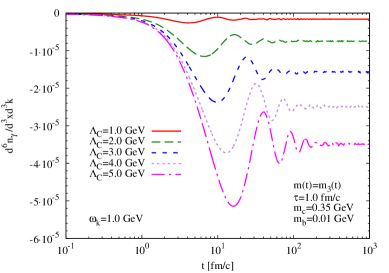
Figure 27: Time evolution of the interference contribution (190b) for $\omega_{\vec{k}}=1\;\mathrm{GeV}$ and different values of $\Lambda_{C}$.

If one first takes $t\rightarrow\infty$, however, it follows from (192) and (193) that these expressions turn into (140) and (143), respectively, so that (190b) vanishes when taking the subsequent limit $\varepsilon\rightarrow 0$.

In addition to the elimination of possible unphysical contributions from (135a) and (135c), keeping the correct sequence of limits is also crucial to obtain physically reasonable results for the contribution from (135b) describing mass-shift effects only. To illustrate this, we show the time evolution of (190a) for different values of $\varepsilon$ in Fig. 28.

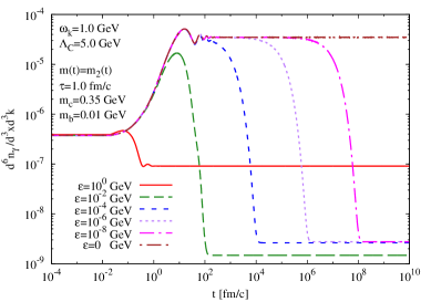
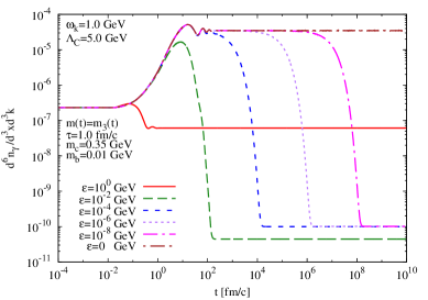
Figure 28: Time evolution of the mass-shift contribution (236) for different values of $\varepsilon$ for $m_{2}(t)$ (left panel) and $m_{3}(t)$ (right panel).

Taking first $\varepsilon\rightarrow 0$ at some finite time, $t$, corresponds to the curve labeled by $\varepsilon=0$ in both panels. If we then take $t\rightarrow\infty$, we obtain an asymptotic value for (190a), which is by several orders of magnitude larger than the one against which the asymptotic values of (190a) for finite $\varepsilon$ converge in the limit $\varepsilon\rightarrow 0$ and which accordingly corresponds to (62). Hence, we have seen that interchanging both limits also leads to unphysical results from the pure mass-shift contribution. Moreover, we see that for sufficiently small values of $\varepsilon$, expression (190a) for finite times $t\geq T\gg\tau$ coincides with its asymptotic value for $\varepsilon=0$. Consequently, the interpretation of (190a) as a photon number at finite times is doubtful as well.

In order to highlight these aspects in particular, we take a closer look at (195) and (144). We see that the integral expressions coincide in both cases whereas the frequency expressions entering (195) feature an additional term of $\text{e}^{\text{i}\omega_{i}t}/\text{i}\omega_{i}$ ($i=0\ldots 4$), which has been eliminated in the corresponding frequency expressions entering (144) after switching off the electromagnetic interaction adiabatically.

In order to see why this additional term is artificial in each case we again consider (190a) for the correct sequence of limits, but instead perform an instantaneous switching of the electromagnetic interaction at $t=\mp 1/\varepsilon$, i.e.,

$$\hat{H}_{\text{EM}}(t)\rightarrow\theta_{\varepsilon}(t)\hat{H}_{\text{EM}}(t)\ ,\quad\text{with}\quad\theta_{\varepsilon}(t)=\theta\left(\frac{1}{\varepsilon^{2}}-t^{2}\right)\quad\text{and}\quad\varepsilon>0\ .$$ (198)

In this case, (143) is replaced by

$$\begin{split}\tilde{I}^{\varepsilon}_{\mu}(\vec{p},\vec{k},r,s)=&\int_{-1/\varepsilon}^{\text{min}(T,1/\varepsilon)}\text{d}t\mbox{ }j^{\text{MST}}_{\mu}(\vec{p},\vec{k},r,s,t)\text{e}^{\text{i}\omega_{\vec{k}}t}\\ -&e\left\{\tilde{\alpha}^{*}_{\vec{p}}\tilde{\gamma}_{\vec{p}+\vec{k}}\bar{u}_{b}(\vec{p},r)\gamma_{\mu}v_{b}(\vec{p}+\vec{k},s)\tilde{g}_{\varepsilon}\left[\omega^{b}_{1}(\vec{p},\vec{k}),T\right]\right.\\ &+\tilde{\alpha}^{*}_{\vec{p}}\tilde{\delta}_{\vec{p}+\vec{k}}\bar{u}_{b}(\vec{p},r)\gamma_{\mu}u_{b}(\vec{p}+\vec{k},s)\tilde{g}^{*}_{\varepsilon}\left[\omega^{b}_{2}(\vec{p},\vec{k}),T\right]\\ &+\tilde{\beta}^{*}_{\vec{p}}\tilde{\gamma}_{\vec{p}+\vec{k}}\bar{v}_{b}(\vec{p},r)\gamma_{\mu}v_{b}(\vec{p}+\vec{k},s)\tilde{g}_{\varepsilon}\left[\omega^{b}_{3}(\vec{p},\vec{k}),T\right]\\ &+\tilde{\beta}^{*}_{\vec{p}}\tilde{\delta}_{\vec{p}+\vec{k}}\bar{v}_{b}(\vec{p},r)\gamma_{\mu}u_{b}(\vec{p}+\vec{k},s)\tilde{g}^{*}_{\varepsilon}\left[\omega^{b}_{4}(\vec{p},\vec{k}),T\right]\\ &-\left.\bar{u}_{c}(\vec{p},r)\gamma_{\mu}v_{c}(\vec{p}+\vec{k},s)\tilde{g}_{\varepsilon}\left[\omega^{c}_{1}(\vec{p},\vec{k}),T\right]\right\}\ .\end{split}$$ (199)

In order to keep the notation more shorthand, we have defined

$$\tilde{g}_{\varepsilon}(\omega,T)=\theta\left(\frac{1}{\varepsilon}-T\right)\frac{\text{e}^{\text{i}\omega/\varepsilon}-\text{e}^{\text{i}\omega T}}{\text{i}\omega}\ .$$ (200)

It follows from (196) and (200) that taking the limit $\varepsilon\rightarrow 0$ in (199) has the same effect as taking $t\rightarrow\infty$ in (195). This can also be inferred from Fig. 29 showing the time evolution of (190a) for different values of $\varepsilon$ with the electromagnetic interaction being switched according to (198).

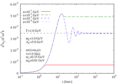
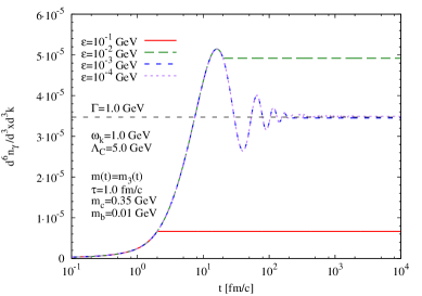
Figure 29: Time evolution of the mass-shift contribution (190a) for $m_{2}(t)$ (left panel) and $m_{3}(t)$ (right panel) with the electromagnetic interaction being switched in terms of (198). If we take the successive limits $t\rightarrow\infty$ and then $\varepsilon\rightarrow 0$, we obtain the same result for (190a) as if we had kept the regularization (44) but interchanged both limits instead. The corresponding value is indicated by the dashed horizontal line in each case.

Thus, if we switch the electromagnetic interaction according to (44) but take the incorrect sequence of limits we obtain the same result for (190a) as if we took the correct sequence of limits but switched the electromagnetic interaction according to (198). This shows us that the former case is formally equivalent to keeping the exact sequence of limits for an unphysical instantaneous switching (198).

In order to emphasize why a switching of the electromagnetic interaction by means of (198) is unphysical, we consider again the Ward-Takahashi identities (61) for the photon self-energy. We have shown in section II and also demonstrated in greater detail in appendix B that these identities are fulfilled when coupling the quark field to a time-dependent scalar background field, $\phi(t)$. But one has to keep in mind that a switching of the electromagnetic interaction leads to a corresponding modification of the photon self-energy, i.e.,

$$\text{i}\Pi^{<}_{\mu\nu}(\vec{k},t_{1},t_{2})\rightarrow\text{i}\Pi^{<,\varepsilon}_{\mu\nu}(\vec{k},t_{1},t_{2})=f_{\varepsilon}(t_{1})f_{\varepsilon}(t_{2})\text{i}\Pi^{<}_{\mu\nu}(\vec{k},t_{1},t_{2})\ ,$$ (201)

with the electromagnetic interaction then being fully persistent at any given time, $t$. Because of the additional factor of $f_{\varepsilon}(t_{1})$, relation (61) is not fulfilled in the first place, but we instead have

$$\partial_{t_{1}}\text{i}\Pi^{<,\varepsilon}_{0\mu}(\vec{k},t_{1},t_{2})-\text{i}k^{j}\text{i}\Pi^{<,\varepsilon}_{j\mu}(\vec{k},t_{1},t_{2})=-\dot{f}_{\varepsilon}(t_{1})f_{\varepsilon}(t_{2})\text{i}\Pi^{<,\varepsilon}_{0\mu}(\vec{k},t_{1},t_{2})\ .$$ (202)

However, if the electromagnetic interaction is switched according to (44), the time derivative reads

$$\dot{f}_{\varepsilon}(t)=\varepsilon\mbox{ sign}(t)\text{e}^{-\varepsilon|t|}\ ,$$ (203)

and, as a consequence, the r.h.s. of (202) vanishes for $\varepsilon\rightarrow 0$ such that (61) is restored again. To the contrary, if we switch the electromagnetic interaction by means of (198), we have no such restoration since

$$\dot{\theta}_{\varepsilon}(t)=\theta\left(\frac{1}{\varepsilon}-t\right)\delta\left(\frac{1}{\varepsilon}+t\right)-\theta\left(\frac{1}{\varepsilon}+t\right)\delta\left(\frac{1}{\varepsilon}-t\right).$$ (204)

Hence, switching the electromagnetic interaction according to (198) effectively leads to a violation of the Ward-Takahashi identities. Since (198) leads to the same asymptotic photon numbers as (44) with the limits being interchanged, we see that the latter procedure also leads to an effective violation of (61).

Appendix D Determination of Bogolyubov parameters $\xi_{\vec{p},s}(t)$ and $\eta_{\vec{p},s}(t)$

In this appendix, we show explicitly that the system of equations (84) for the Bogolyubov parameters, $\xi_{\vec{p},s}(t)$ and $\eta_{\vec{p},s}(t)$, is solved by (85). For this purpose, we first rewrite the fermionic field operator, $\hat{\psi}(x)$, in terms of the transformed operators (71), i.e.,

$$\hat{\psi}(x)=\sum_{s}\int\frac{\text{d}^{3}p}{(2\pi)^{3}}\left[\hat{\tilde{b}}_{\vec{p},s}(t)\tilde{\psi}_{\vec{p},s,\uparrow}(x)+\hat{\tilde{d}}^{\dagger}_{-\vec{p},s}(t)\tilde{\psi}_{\vec{p},s\downarrow}(x)\right]\ .$$ (205)

Here we have made use of (76) and introduced the transformed positive and negative energy wavefunctions

$$\tilde{\psi}_{\vec{p},s,\uparrow}(x) = \xi^{*}_{\vec{p},s}(t)\psi_{\vec{p},s\uparrow}(x)+\eta^{*}_{\vec{p},s}(t)\psi_{\vec{p},s\downarrow}(x)\ ,$$ (206a)

$$\tilde{\psi}_{\vec{p},s,\downarrow}(x) = \xi_{\vec{p},s}(t)\psi_{\vec{p},s\downarrow}(x)-\eta_{\vec{p},s}(t)\psi_{\vec{p},s\uparrow}(x)\ .$$ (206b)

It follows from (72) that the inverse transformation relations are given by

$$\psi_{\vec{p},s,\uparrow}(x) = \xi_{\vec{p},s}(t)\tilde{\psi}_{\vec{p},s\uparrow}(x)-\eta^{*}_{\vec{p},s}(t)\tilde{\psi}_{\vec{p},s\downarrow}(x)\ ,$$ (207a)

$$\psi_{\vec{p},s,\downarrow}(x) = \xi^{*}_{\vec{p},s}(t)\tilde{\psi}_{\vec{p},s\downarrow}(x)+\eta_{\vec{p},s}(t)\tilde{\psi}_{\vec{p},s\uparrow}(x)\ .$$ (207b)

Now the strategy is to rewrite (84) as matrix-element conditions for $\tilde{\psi}_{\vec{p},s\uparrow\downarrow}(x)$ from which the latter are determined. The corresponding Bogolyubov parameters, $\xi_{\vec{p},s}(t)$ and $\eta_{\vec{p},s}(t)$, are then given by

$$\xi_{\vec{p},s}(t)=\quad\psi^{\dagger}_{\vec{p},s\downarrow}(x)\tilde{\psi}_{\vec{p},s\downarrow}(x) =\left[\psi^{\dagger}_{\vec{p},s\uparrow}(x)\tilde{\psi}_{\vec{p},s\uparrow}(x)\right]^{*}=\tilde{\psi}^{\dagger}_{\vec{p},s\uparrow}(x)\psi_{\vec{p},s\uparrow}(x)\ ,$$ (208a)

$$\eta_{\vec{p},s}(t)=-\psi^{\dagger}_{\vec{p},s\uparrow}(x)\tilde{\psi}_{\vec{p},s\downarrow}(x) =\left[\psi^{\dagger}_{\vec{p},s\downarrow}(x)\tilde{\psi}_{\vec{p},s\uparrow}(x)\right]^{*}=\tilde{\psi}^{\dagger}_{\vec{p},s\uparrow}(x)\psi_{\vec{p},s\downarrow}(x)\ .$$ (208b)

Expressing (68a)-(68b) in terms of (207a)-(207b) and making use of (72), we can rewrite (84) in terms of $\tilde{\psi}_{\vec{p},s\uparrow\downarrow}(x)$ as

$$\xi_{\vec{p},s}(t)\mbox{ }\tilde{\psi}^{\dagger}_{\vec{p},s,\uparrow}(x)\hat{h}_{D}(t)\tilde{\psi}_{\vec{p},s,\uparrow}(x)-\eta^{*}_{\vec{p},s}(t)\mbox{ }\tilde{\psi}^{\dagger}_{\vec{p},s,\uparrow}(x)\hat{h}_{D}(t)\tilde{\psi}_{\vec{p},s,\downarrow}(x) =E_{\vec{p}}(t)\xi_{\vec{p},s}(t)\ ,$$ (209a)

$$-\eta_{\vec{p},s}(t)\mbox{ }\tilde{\psi}^{\dagger}_{\vec{p},s,\downarrow}(x)\hat{h}_{D}(t)\tilde{\psi}_{\vec{p},s,\downarrow}(x)+\xi^{*}_{\vec{p},s}(t)\mbox{ }\tilde{\psi}^{\dagger}_{\vec{p},s,\uparrow}(x)\hat{h}_{D}(t)\tilde{\psi}_{\vec{p},s,\downarrow}(x) =E_{\vec{p}}(t)\eta_{\vec{p},s}(t)\ ,$$ (209b)

To keep the notation short, we have introduced

$$\hat{h}_{D}(t)=-\text{i}\gamma_{0}\vec{\gamma}\cdot\vec{\nabla}+\gamma_{0}m(t)\ .$$ (210)

Taking into account that

$$\tilde{\psi}^{\dagger}_{\vec{p},s,\downarrow}(x)\hat{h}_{D}(t)\tilde{\psi}_{\vec{p},s,\downarrow}(x)=-\tilde{\psi}^{\dagger}_{\vec{p},s,\uparrow}(x)\hat{h}_{D}(t)\tilde{\psi}_{\vec{p},s,\uparrow}(x)\ ,$$ (211)

which follows from (206) and (68a), one can show that (209a)-(209b) are equivalent to

$$\tilde{\psi}^{\dagger}_{\vec{p},s,\uparrow}(x)\hat{h}_{D}(t)\tilde{\psi}_{\vec{p},s,\uparrow}(x) = E_{\vec{p}}(t)\ ,$$ (212a)

$$\tilde{\psi}^{\dagger}_{\vec{p},s,\uparrow}(x)\hat{h}_{D}(t)\tilde{\psi}_{\vec{p},s,\downarrow}(x) = 0\ .$$ (212b)

The Bogolyubov transformation (71) hence corresponds to a reexpansion of the fermion-field operators in terms of the instantaneous eigenstates of the Hamilton-density operator (210). In order to solve Eqs. (212a)-(212b) for the matrix elements, we parametrize $\tilde{\psi}_{\vec{p},s\uparrow\downarrow}(x)$ analogously to (35) as

$$\tilde{\psi}_{\vec{p},s,\uparrow\downarrow}(x)=\begin{pmatrix}\tilde{\alpha}_{\vec{p},\uparrow\downarrow}(t)\chi_{s}\\ \tilde{\beta}_{\vec{p},\uparrow\downarrow}(t)\frac{\vec{\sigma}\cdot\vec{p}}{p}\chi_{s}\end{pmatrix}e^{\text{i}\vec{p}\cdot\vec{x}}\text{.}$$ (213)

Writing (206a) and (206b) in terms of wavefunction parameters, it follows from (38) and (72) that

$$\left|\tilde{\alpha}_{\vec{p},\uparrow\downarrow}(t)\right|^{2}+\left|\tilde{\beta}_{\vec{p},\uparrow\downarrow}(t)\right|^{2}=1\ .$$ (214)

Furthermore, relations (39) imply

$$\tilde{\alpha}_{\vec{p},\downarrow}(t) = \tilde{\beta}^{*}_{\vec{p},\uparrow}(t)\ ,$$ (215a)

$$\tilde{\beta}_{\vec{p},\downarrow}(t) = -\tilde{\alpha}^{*}_{\vec{p},\uparrow}(t)\ .$$ (215b)

Upon insertion of (213) into (212a)-(212b) and making use of (215a)-(215b) the diagonalization conditions can be written as

$$p\left(\tilde{\alpha}^{*}_{\vec{p},\uparrow}(t)\tilde{\beta}_{\vec{p},\uparrow}(t)+\tilde{\alpha}_{\vec{p},\uparrow}(t)\tilde{\beta}^{*}_{\vec{p},\uparrow}(t)\right)+m(t)\left(\left|\tilde{\alpha}_{\vec{p},\uparrow}(t)\right|^{2}-\left|\tilde{\beta}_{\vec{p},\uparrow}(t)\right|^{2}\right)= E_{\vec{p}}(t)\ ,$$ (216a)

$$p\left(\tilde{\beta}^{2}_{\vec{p},\uparrow}(t)-\tilde{\alpha}^{2}_{\vec{p},\uparrow}(t)\right)+2m(t)\tilde{\alpha}_{\vec{p},\uparrow}(t)\tilde{\beta}_{\vec{p},\uparrow}(t)= 0\ .$$ (216b)

Expressing the wavefunction parameters in terms of polar coordinates, i.e.,

$$\tilde{\alpha}_{\vec{p},\uparrow}(t) = \left|\tilde{\alpha}_{\vec{p},\uparrow}(t)\right|e^{\text{i}\phi_{\alpha}}\ ,$$ (217a)

$$\tilde{\beta}_{\vec{p},\uparrow}(t) = \left|\tilde{\beta}_{\vec{p},\uparrow}(t)\right|e^{\text{i}\phi_{\beta}}\ ,$$ (217b)

and taking into account that the l.h.s.s of both (216a) and (216b) are real valued, one obtains

$$\sin\left[\phi_{\alpha}(t)-\phi_{\beta}(t)\right] = 0\ ,$$

$$\cos\left[\phi_{\alpha}(t)-\phi_{\beta}(t)\right] = (-1)^{n}\ .$$

Therefore, we can rewrite (216a)-(216b) as

$$(-1)^{n}2p\left|\tilde{\alpha}_{\vec{p},\uparrow}(t)\right|\left|\tilde{\beta}_{\vec{p},\uparrow}(t)\right|+m(t)\left(\left|\tilde{\alpha}_{\vec{p},\uparrow}(t)\right|^{2}-\left|\tilde{\beta}_{\vec{p},\uparrow}(t)\right|^{2}\right) = E_{\vec{p}}(t)\ ,$$ (218a)

$$(-1)^{n}p\left(\left|\tilde{\alpha}_{\vec{p},\uparrow}(t)\right|^{2}-\left|\tilde{\beta}_{\vec{p},\uparrow}(t)\right|^{2}\right)+2m(t)\left|\tilde{\alpha}_{\vec{p},\uparrow}(t)\right|\left|\tilde{\beta}_{\vec{p},\uparrow}(t)\right| = 0\ ,$$ (218b)

which is equivalent to

$$\left|\tilde{\alpha}_{\vec{p},\uparrow}(t)\right|\left|\tilde{\beta}_{\vec{p},\uparrow}(t)\right| = (-1)^{n}\frac{p}{2E_{\vec{p}}(t)}\ ,$$ (219a)

$$\left|\tilde{\alpha}_{\vec{p},\uparrow}(t)\right|^{2}-\left|\tilde{\beta}_{\vec{p},\uparrow}(t)\right|^{2} = \frac{m(t)}{E_{\vec{p}}(t)}\ .$$ (219b)

Relation (219a) implies that $n$ must be even. Thus, without loss of generality, we can assume that $\phi_{\alpha}(t)=\phi_{\beta}(t)\equiv\phi(t)$. Together with the normalization condition (214), it follows from (219a)-(219b) that we have

$$\tilde{\alpha}_{\vec{p},\uparrow}(t) = \sqrt{\frac{E_{\vec{p}}(t)+m(t)}{2E_{\vec{p}}(t)}}e^{\text{i}\phi(t)}\ ,$$ (220a)

$$\tilde{\beta}_{\vec{p},\uparrow}(t) = \sqrt{\frac{E_{\vec{p}}(t)-m(t)}{2E_{\vec{p}}(t)}}e^{\text{i}\phi(t)}\ .$$ (220b)

Since $\psi_{\vec{p},s,\uparrow\downarrow}(x)$ and $\tilde{\psi}_{\vec{p},s,\uparrow\downarrow}(x)$ coincide with each other for $t\leq t^{{}^{\prime}}_{0}$, $\phi(t)$ can, in principle, be chosen freely as long as it fulfills the asymptotic condition $\phi(t)\rightarrow E^{c}_{\vec{p}}t$ for $t\rightarrow-\infty$. It is hence convenient to choose $\phi(t)=E_{\vec{p}}(t)t$ so that our Bogolyubov transformation corresponds to an expansion of $\hat{\psi}(x)$ in terms of positive and negative energy wavefunctions of the respective current mass, $m(t)$. As a consequence, we finally have for the transformed positive and negative energy wavefunction parameters

$$\tilde{\alpha}_{\vec{p},\uparrow}(t) = \sqrt{\frac{E_{\vec{p}}(t)+m(t)}{2E_{\vec{p}}(t)}}e^{\text{i}E_{\vec{p}}(t)t}\ ,$$ (221a)

$$\tilde{\beta}_{\vec{p},\uparrow}(t) = \sqrt{\frac{E_{\vec{p}}(t)-m(t)}{2E_{\vec{p}}(t)}}e^{\text{i}E_{\vec{p}}(t)t}\ ,$$ (221b)

$$\tilde{\alpha}_{\vec{p},\downarrow}(t) = \sqrt{\frac{E_{\vec{p}}(t)-m(t)}{2E_{\vec{p}}(t)}}e^{-\text{i}E_{\vec{p}}(t)t}\ ,$$ (221c)

$$\tilde{\beta}_{\vec{p},\downarrow}(t) = -\sqrt{\frac{E_{\vec{p}}(t)+m(t)}{2E_{\vec{p}}(t)}}e^{-\text{i}E_{\vec{p}}(t)t}\ ,$$ (221d)

and hence

$$\xi_{\vec{p},s}(t) = e^{\text{i}E_{\vec{p}}(t)t}\left[\sqrt{\frac{E_{\vec{p}}(t)+m(t)}{2E_{\vec{p}}(t)}}\alpha_{\vec{p},\uparrow}(t)+\sqrt{\frac{E_{\vec{p}}(t)-m(t)}{2E_{\vec{p}}(t)}}\beta_{\vec{p},\uparrow}(t)\right]\ ,$$ (222a)

$$\eta_{\vec{p},s}(t) = e^{\text{i}E_{\vec{p}}(t)t}\left[\sqrt{\frac{E_{\vec{p}}(t)+m(t)}{2E_{\vec{p}}(t)}}\alpha_{\vec{p},\downarrow}(t)+\sqrt{\frac{E_{\vec{p}}(t)-m(t)}{2E_{\vec{p}}(t)}}\beta_{\vec{p},\downarrow}(t)\right]\ .$$ (222b)

These are just the Bogolyubov parameters (85).

Appendix E Evaluation of $I_{ij}(\vec{p},\vec{k})$

In this appendix, we demonstrate how to evaluate $I_{ij}(\vec{p},\vec{k})$ ($i,j=1..4$), which characterize the direct contributions from first-order QED processes (equal indices) and their interference among each other (different indices). We will carry out the calculations explicitly for one direct contribution and one interference contribution, respectively. The evaluation of the remaining contributions proceeds analogously. In order to calculate the direct contribution from the spontaneous creation of a quark-antiquark pair together with a photon, $I_{11}(\vec{p},\vec{k})$, we first recall that the corresponding transition amplitude is given by

$$I^{1}_{\mu}(\vec{p},\vec{k},r,s)=\text{i}e\alpha_{\vec{p}}\alpha_{\vec{p}+\vec{k}}\bar{u}_{b}(\vec{p},r)\gamma_{\mu}v_{b}(\vec{p}+\vec{k},s)\left(\frac{1}{\omega^{b}_{1}(\vec{p},\vec{k})}-\frac{1}{\omega^{c}_{1}(\vec{p},\vec{k})}\right)^{2}\ .$$ (223)

In order to carry out the spin summation in $I_{11}(\vec{p},\vec{k})$, we take into account that

$$\sum_{s}u_{b}(\vec{p},s)\bar{u}_{b}(\vec{p},s)=\frac{\not{p}+m_{b}}{2E^{b}_{\vec{p}}}\ ,$$ (224a)

$$\sum_{s}v_{b}(\vec{p},s)\bar{v}_{b}(\vec{p},s)=\frac{\not{\bar{p}}-m_{b}}{2E^{b}_{\vec{p}}}\ ,$$ (224b)

where $\bar{p}^{\mu}=(E^{b}_{\vec{p}},-\vec{p})$. Hence, $I_{11}(\vec{p},\vec{k})$ can be rewritten as

$$I_{11}(\vec{p},\vec{k})=e^{2}\frac{\gamma^{\mu\nu}(k)\alpha^{2}_{\vec{p}+\vec{k}}\alpha^{2}_{\vec{p}}}{4E^{b}_{\vec{p}+\vec{k}}E^{b}_{\vec{p}}}\left(\frac{1}{\omega^{b}_{1}(\vec{p},\vec{k})}-\frac{1}{\omega^{c}_{1}(\vec{p},\vec{k})}\right)^{2}\cdot\mbox{Tr}\left\{\gamma_{\nu}(\not{\bar{q}}-m_{b})\gamma_{\mu}(\not{p}+m_{b})\right\}\ .$$ (225)

where we have introduced $q^{\mu}=(E^{b}_{\vec{p}+\vec{k}},\vec{p}+\vec{k})$. Using standard Dirac trace techniques, we find that

$$\mbox{Tr}\left\{\gamma_{\nu}(\not{\bar{q}}-m_{b})\gamma_{\mu}(\not{p}+m_{b})\right\}=4\left[\bar{q}_{\nu}p_{\mu}+\bar{q}_{\mu}p_{\nu}-\eta_{\nu\mu}\left(\bar{q}\cdot p+m^{2}_{b}\right)\right]\ .$$ (226)

Taking into account that $\gamma^{\mu\nu}(k)$ has a purely spacelike structure given by (48), carrying out the contraction entering (225) finally yields

$$I_{11}(\vec{p},\vec{k},t)=2e^{2}\alpha^{2}_{\vec{p}+\vec{k}}\alpha^{2}_{\vec{p}}\left(1+\frac{px(px+\omega_{\vec{k}})+m^{2}_{b}}{E^{b}_{\vec{p}+\vec{k}}E^{b}_{\vec{p}}}\right)\left(\frac{1}{\omega^{b}_{1}(\vec{p},\vec{k})}-\frac{1}{\omega^{c}_{1}(\vec{p},\vec{k})}\right)^{2}\ .$$ (227)

The evaluation of the direct contributions from quark and antiquark bremsstrahlung and quark-antiquark annihilation into a photon is performed in the same way. Next, we turn to the evaluation of the interference contributions. In its course, we encounter spin summations over mixed tensor products between positive- and negative-energy spinors. These evaluate to

$$\sum_{s}u_{b}(\vec{p},s)\bar{v}_{b}(\vec{p},s)=-\frac{(\not{p}+m_{b})\not{n}_{\vec{p}}}{2E^{b}_{p}}\ ,$$ (228a)

$$\sum_{s}v_{b}(\vec{p},s)\bar{u}_{b}(\vec{p},s)=-\frac{\not{n}_{\vec{p}}(\not{p}+m_{b})}{2E^{b}_{p}}\ ,$$ (228b)

where we have introduced $n^{\mu}_{\vec{p}}=(0,\vec{p}/p)$ and taken into account that

$$\not{n}_{\vec{p}}u_{b}(\vec{p},s) = -v_{b}(\vec{p},s)\ ,$$ (229a)

$$\not{n}_{\vec{p}}v_{b}(\vec{p},s) = u_{b}(\vec{p},s)\ .$$ (229b)

With help of these relations, the contribution describing the interference between the spontaneous creation of a quark/antiquark pair together with a photon and quark pair annihilation into a photon, $I_{14}(\vec{p},\vec{k},t)$, can be rewritten as

$$I_{14}(\vec{p},\vec{k})= e^{2}\frac{\alpha_{\vec{p}}\beta_{\vec{p}}\alpha_{\vec{p}+\vec{k}}\beta_{\vec{p}+\vec{k}}}{4E^{b}_{\vec{p}}E^{b}_{\vec{p}+\vec{k}}}\left(\frac{1}{\omega^{b}_{1}(\vec{p},\vec{k})}-\frac{1}{\omega^{c}_{1}(\vec{p},\vec{k})}\right)\left(\frac{1}{\omega^{b}_{4}(\vec{p},\vec{k})}+\frac{1}{\omega^{c}_{1}(\vec{p},\vec{k})}\right)$$

$$\cdot\mbox{Tr}\left\{\gamma_{\nu}(\not{p}+\not{k}+m_{b})\not{n}_{\vec{p}+\vec{k}}\gamma_{\mu}(\not{p}+m_{b})\not{n}_{\vec{p}}\right\}$$ (230)

Thus, in contrast to the direct contributions, carrying out the spin summations for the interference contributions gives rise to traces over products of six Dirac matrices. Making use of the anticommutation relation

$$\left\{\gamma^{\mu},\gamma^{\nu}\right\}=2\eta^{\mu\nu}$$

and cyclic trace invariance, these traces can be reduced to

$$\mbox{Tr}\left\{\gamma^{\alpha}\gamma^{\beta}\gamma^{\gamma}\gamma^{\delta}\gamma^{\epsilon}\gamma^{\zeta}\right\} = \eta^{\alpha\beta}\mbox{Tr}\left\{\gamma^{\gamma}\gamma^{\delta}\gamma^{\epsilon}\gamma^{\zeta}\right\}-\eta^{\alpha\gamma}\mbox{Tr}\left\{\gamma^{\beta}\gamma^{\delta}\gamma^{\epsilon}\gamma^{\zeta}\right\}+$$ (231)

$$\eta^{\alpha\delta}\mbox{Tr}\left\{\gamma^{\beta}\gamma^{\gamma}\gamma^{\epsilon}\gamma^{\zeta}\right\}-\eta^{\alpha\epsilon}\mbox{Tr}\left\{\gamma^{\beta}\gamma^{\gamma}\gamma^{\delta}\gamma^{\zeta}\right\}+$$

$$\eta^{\alpha\zeta}\mbox{Tr}\left\{\gamma^{\beta}\gamma^{\gamma}\gamma^{\delta}\gamma^{\epsilon}\right\}\ .$$

With the help of (231), the trace entering (E) is evaluated to

$$\begin{split}\mathrm{Tr}&\left\{\gamma_{\nu}(\not{p}+\not{k}+m_{b})\not{n}_{\vec{p}+\vec{k}}\gamma_{\mu}(\not{p}+m_{b})\not{n}_{\vec{p}}\right\}\\ &=\frac{E^{b}_{\vec{p}}E^{b}_{\vec{p}+\vec{k}}}{p|\vec{p}+\vec{k}|}\left[p_{i}(p_{j}+k_{j})+p_{j}(p_{i}+k_{i})+\eta_{ij}\vec{p}\cdot(\vec{p}+\vec{k})\right]+\eta_{ij}p|\vec{p}+\vec{k}|\ .\end{split}$$ (232)

We have considered only spacelike indices since the trace expression entering (E) is still contracted with $\gamma^{\mu\nu}(k)$ which has an exclusively spacelike structure. This contraction leads to

$$\gamma^{\mu\nu}(k)\mbox{Tr}\left\{\gamma_{\nu}(\not{p}+\not{k}+m_{b})\not{n}_{\vec{p}+\vec{k}}\gamma_{\mu}(\not{p}+m_{b})\not{n}_{\vec{p}}\right\}$$

$$= -8p^{2}|\vec{p}+\vec{k}|^{2}\left(1+\frac{px(px+\omega_{\vec{k}})(E^{b}_{\vec{p}}E^{b}_{\vec{p}+\vec{k}}-m^{2}_{b})}{|\vec{p}+\vec{k}|^{2}}\right)\ ,$$ (233)

so that (E) finally reads

$$\begin{split}I_{14}(\vec{p},\vec{k})=&-2e^{2}\frac{\alpha_{\vec{p}}\beta_{\vec{p}}\alpha_{\vec{p}+\vec{k}}\beta_{\vec{p}+\vec{k}}}{4E^{b}_{\vec{p}}E^{b}_{\vec{p}+\vec{k}}}p|\vec{p}+\vec{k}|\left(1+\frac{(px(px+\omega_{\vec{k}}))(E^{b}_{\vec{p}}E^{b}_{\vec{p}+\vec{k}}-m^{2}_{b})}{|\vec{p}+\vec{k}|^{2}}\right)\\ &\cdot\left(\frac{1}{\omega^{b}_{1}(\vec{p},\vec{k})}-\frac{1}{\omega^{c}_{1}(\vec{p},\vec{k})}\right)\left(\frac{1}{\omega^{b}_{4}(\vec{p},\vec{k})}+\frac{1}{\omega^{c}_{1}(\vec{p},\vec{k})}\right)\ .\end{split}$$ (234)

The evaluation of the remaining interference contributions follows the same steps. After evaluating all direct and interference contributions the substitutions $\vec{p}\rightarrow\vec{p}-\vec{k}$ and $x\rightarrow-1$ show that the remaining integration over $\text{d}^{3}p$ yields the same contribution for $I_{22}(\vec{p},\vec{k},t)$ and $I_{33}(\vec{p},\vec{k},t)$, for $I_{12}(\vec{p},\vec{k},t)$ and $I_{13}(\vec{p},\vec{k},t)$ and for $I_{24}(\vec{p},\vec{k},t)$ and $I_{34}(\vec{p},\vec{k},t)$. For that reason, theses contributions have been taken together as shown in (128) in each case.

Appendix F Remarks on $m_{b}=0$ for an instantaneous mass shift

In this appendix, we discuss the special case of $m_{b}=0$ for an instantaneous mass shift. It requires some special considerations since the frequencies describing quark/antiquark bremsstrahlung and pair annihilation into a photon are no longer negative or positive definite. We first take into account that we have

$$\alpha_{\vec{p}} = \frac{1}{\sqrt{2}}\left(\cos\varphi^{c}_{\vec{p}}+\sin\varphi^{c}_{\vec{p}}\right)\ ,$$ (235a)

$$\beta_{\vec{p}} = \frac{1}{\sqrt{2}}\left(\cos\varphi^{c}_{\vec{p}}-\sin\varphi^{c}_{\vec{p}}\right)\ ,$$ (235b)

for $m_{b}=0$. The asymptotic direct contributions hence turn into:

$$I_{11}(\vec{p},\vec{k})=\frac{e^{2}}{2} \left(1+\frac{|\vec{p}+\vec{k}|}{E^{c}_{\vec{p}+\vec{k}}}\right)\left(1+\frac{p}{E^{c}_{\vec{p}}}\right)\left(1+\frac{x(px+\omega_{\vec{k}})}{|\vec{p}+\vec{k}|}\right)$$

$$\times \left(\frac{1}{|\vec{p}+\vec{k}|+p+\omega_{\vec{k}}}-\frac{1}{E^{c}_{\vec{p}+\vec{k}}+E^{c}_{\vec{p}}+\omega_{\vec{k}}}\right)^{2}\ ,$$ (236a)

$$\tilde{I}_{22}(\vec{p},\vec{k})=e^{2} \left(1-\frac{|\vec{p}+\vec{k}|}{E^{c}_{\vec{p}+\vec{k}}}\right)\left(1+\frac{p}{E^{c}_{\vec{p}}}\right)\left(1-\frac{x(px+\omega_{\vec{k}})}{|\vec{p}+\vec{k}|}\right)$$

$$\times \left(\frac{1}{|\vec{p}+\vec{k}|-p-\omega_{\vec{k}}}+\frac{1}{E^{c}_{\vec{p}+\vec{k}}+E^{c}_{\vec{p}}+\omega_{\vec{k}}}\right)^{2}\ ,$$ (236b)

$$I_{44}(\vec{p},\vec{k})=\frac{e^{2}}{2} \left(1-\frac{|\vec{p}+\vec{k}|}{E^{c}_{\vec{p}+\vec{k}}}\right)\left(1-\frac{p}{E^{c}_{\vec{p}}}\right)\left(1+\frac{x(px+\omega_{\vec{k}})}{|\vec{p}+\vec{k}|}\right)$$

$$\times \left(\frac{1}{|\vec{p}+\vec{k}|+p-\omega_{\vec{k}}}+\frac{1}{E^{c}_{\vec{p}+\vec{k}}+E^{c}_{\vec{p}}+\omega_{\vec{k}}}\right)^{2}\ .$$ (236c)

Furthermore, it follows from (127) that $\tilde{I}_{12}(\vec{p},\vec{k})$ and $\tilde{I}_{24}(\vec{p},\vec{k})$ vanish for $m_{b}=0$ and the remaining interference contributions simplify to

$$I_{14}(\vec{p},\vec{k})=-\frac{e^{2}}{2E^{c}_{\vec{p}}E^{c}_{\vec{p}+\vec{k}}}\left(1+\frac{x(px+\omega_{\vec{k}})}{|\vec{p}+\vec{k}|}\right) \left(\frac{1}{|\vec{p}+\vec{k}|+p+\omega_{\vec{k}}}-\frac{1}{E^{c}_{\vec{p}+\vec{k}}+E^{c}_{\vec{p}}+\omega_{\vec{k}}}\right)$$

$$\cdot \left(\frac{1}{|\vec{p}+\vec{k}|+p-\omega_{\vec{k}}}+\frac{1}{E^{c}_{\vec{p}+\vec{k}}+E^{c}_{\vec{p}}+\omega_{\vec{k}}}\right)\ ,$$ (237a)

$$I_{23}(\vec{p},\vec{k})=-\frac{e^{2}}{2E^{c}_{\vec{p}}E^{c}_{\vec{p}+\vec{k}}}\left(1-\frac{x(px+\omega_{\vec{k}})}{|\vec{p}+\vec{k}|}\right) \left(\frac{1}{|\vec{p}+\vec{k}|-p-\omega_{\vec{k}}}+\frac{1}{E^{c}_{\vec{p}+\vec{k}}+E^{c}_{\vec{p}}+\omega_{\vec{k}}}\right)$$

$$\cdot \left(\frac{1}{|\vec{p}+\vec{k}|-p+\omega_{\vec{k}}}-\frac{1}{E^{c}_{\vec{p}+\vec{k}}+E^{c}_{\vec{p}}+\omega_{\vec{k}}}\right)\ .$$ (237b)

Since the frequencies describing quark/antiquark bremsstrahlung and pair annihilation into a photon are no longer negative or positive definite, we have to investigate, whether the loop integral features possible infrared ($p\rightarrow 0$) and/or (anti-) collinear ($x\rightarrow\pm 1$) singularities. In the limit $p\rightarrow 0$, they behave as

$$I_{11}(\vec{p},\vec{k}) \rightarrow \frac{e^{2}(1+x)}{2}\left(1+\frac{\omega_{\vec{k}}}{\sqrt{\omega_{\vec{k}}^{2}+m^{2}_{c}}}\right)\left(\frac{1}{2\omega_{\vec{k}}}-\frac{1}{\sqrt{\omega^{2}_{\vec{k}}+m^{2}_{c}}+E^{c}_{\vec{p}}+\omega_{\vec{k}}}\right)^{2}+\mathcal{O}(p)\ ,$$ (238a)

$$\tilde{I}_{22}(\vec{p},\vec{k}) \rightarrow e^{2}\left(1-\frac{\omega_{\vec{k}}}{\sqrt{\omega_{\vec{k}}^{2}+m^{2}_{c}}}\right)\frac{1}{p^{2}(1-x)}+\mathcal{O}\left(\frac{1}{p}\right)\ ,$$ (238b)

$$I_{44}(\vec{p},\vec{k}) \rightarrow \frac{e^{2}}{2}\left(1-\frac{\omega_{\vec{k}}}{\sqrt{\omega_{\vec{k}}^{2}+m^{2}_{c}}}\right)\frac{1}{p^{2}(1+x)}+\mathcal{O}\left(\frac{1}{p}\right)\ ,$$ (238c)

$$I_{14}(\vec{p},\vec{k}) \rightarrow -\frac{e^{2}}{2}\frac{m_{c}}{p\sqrt{\omega_{\vec{k}}^{2}+m^{2}_{c}}}\left(\frac{1}{2\omega_{\vec{k}}}-\frac{1}{\sqrt{\omega^{2}_{\vec{k}}+m^{2}_{c}}+E^{c}_{\vec{p}}+\omega_{\vec{k}}}\right)+\mathcal{O}(1)\ ,$$ (238d)

$$I_{23}(\vec{p},\vec{k}) \rightarrow \frac{e^{2}}{2}\frac{m_{c}}{p\sqrt{\omega_{\vec{k}}^{2}+m^{2}_{c}}}\left(\frac{1}{2\omega_{\vec{k}}}-\frac{1}{\sqrt{\omega^{2}_{\vec{k}}+m^{2}_{c}}+E^{c}_{\vec{p}}+\omega_{\vec{k}}}\right)+\mathcal{O}(1)\ .$$ (238e)

Since the integration measure $\text{d}^{3}p$ contributes an additional factor of $p^{2}$ to each contribution, no infrared singularities will show up in the loop integral for $m_{b}=0$. As a next step, we consider the collinear limit $x\rightarrow 1$. In this limit, the direct contribution from quark/antiquark bremsstrahlung turns into

$$\tilde{I}_{22}(\vec{p},\vec{k})\rightarrow-e^{2}\left.\left(1-\frac{|\vec{p}+\vec{k}|}{E^{c}_{\vec{p}+\vec{k}}}\right)\right|_{x=1}\left(1+\frac{p}{E^{c}_{\vec{p}}}\right)\frac{(p+\omega_{\vec{k}})^{2}+p^{2}}{p^{2}\omega_{\vec{k}}^{2}(x-1)}+\mathcal{O}(1)$$ (239)

with all other contributions staying finite. Furthermore, the direct contribution from pair annihilation into a photon features an anti-collinear singularity in the limit $x\rightarrow\-1$ if $p<\omega_{\vec{k}}$, i.e.,

$$I_{44}(\vec{p},\vec{k})\rightarrow\frac{e^{2}}{2}\left.\left(1-\frac{|\vec{p}+\vec{k}|}{E^{c}_{\vec{p}+\vec{k}}}\right)\right|_{x=-1}\left(1-\frac{p}{E^{c}_{\vec{p}}}\right)\frac{(p-\omega_{\vec{k}})^{2}+p^{2}}{p^{2}\omega_{\vec{k}}^{2}(x+1)}+\mathcal{O}(1)\ .$$ (240)

For $p>\omega_{\vec{k}}$, $I_{44}(\vec{p},\vec{k},t)$ stays finite for $x\rightarrow-1$. All other contributions generally stay finite in that limit. Therefore, in the limit $m_{b}\rightarrow 0$, the loop integral develops a collinear and an anticollinear singularity for the contributions from quark/antiquark Bremsstrahlung and quark pair annihilation into a photon, respectively.

References

- Bali and Schilling (1992) G. S. Bali and K. Schilling, Phys. Rev. D 46, 2626 (1992).
- Gross and Wilczek (1973) D. Gross and F. Wilczek, Phys. Rev. Lett. 30, 1343 (1973).
- Politzer (1973) H. D. Politzer, Phys. Rev. Lett. 30, 1346 (1973).
- Shuryak (1978a) E. V. Shuryak, Phys. Lett. B 78, 150 (1978a).
- Shuryak (1978b) E. V. Shuryak, Sov. Phys. JETP 47, 212 (1978b).
- Yagi et al. (2005) K. Yagi, T. Hatsuda, and Y. Miake, Camb. Monogr. Part. Phys. Nucl. Phys. Cosmol. 23, 1 (2005).
- Müller and Nagle (2006) B. Müller and J. L. Nagle, Ann. Rev. Nucl. Part. Sci. 56, 93 (2006).
- Friman et al. (2011) B. Friman et al., Lect. Notes Phys. 814, 1 (2011).
- Schwinger (1961) J. S. Schwinger, J. Math. Phys. 2, 407 (1961).
- Bakshi and Mahanthappa (1963a) P. M. Bakshi and K. T. Mahanthappa, J. Math. Phys. 4, 1 (1963a).
- Bakshi and Mahanthappa (1963b) P. M. Bakshi and K. T. Mahanthappa, J. Math. Phys. 4, 12 (1963b).
- Keldysh (1964) L. Keldysh, Zh. Eks. Theor. Fiz. 47, 1515 (1964), [Sov. Phys. JETP 20, 1018 (1965)].
- Craig (1968) R. Craig, J. Math. Phys. 9, 605 (1968).
- Danielewicz (1984a) P. Danielewicz, Ann. Phys. 152, 239 (1984a).
- Chou et al. (1985) K.-c. Chou, Z.-b. Su, B.-l. Hao, and L. Yu, Phys. Rept. 118, 1 (1985).
- Landsman and van Weert (1987) N. Landsman and C. van Weert, Phys. Rept. 145, 141 (1987).
- Greiner and Leupold (1998) C. Greiner and S. Leupold, Ann. Phys. 270, 328 (1998).
- Berges (2002) J. Berges, Nucl. Phys. A 699, 847 (2002).
- Nahrgang et al. (2011) M. Nahrgang, S. Leupold, C. Herold, and M. Bleicher, Phys. Rev. C 84, 024912 (2011).
- Nahrgang et al. (2012) M. Nahrgang, S. Leupold, and M. Bleicher, Phys. Lett. B 711, 109 (2012).
- Danielewicz (1984b) P. Danielewicz, Ann. Phys. 152, 305 (1984b).
- Greiner et al. (1994) C. Greiner, K. Wagner, and P. G. Reinhard, Phys. Rev. C 49, 1693 (1994).
- Kohler (1995) H. S. Kohler, Phys. Rev. C 51, 3232 (1995).
- Xu and Greiner (2000) Z. Xu and C. Greiner, Phys. Rev. D 62, 036012 (2000).
- Juchem et al. (2004a) S. Juchem, W. Cassing, and C. Greiner, Nucl. Phys. A 743, 92 (2004a).
- Juchem et al. (2004b) S. Juchem, W. Cassing, and C. Greiner, Phys. Rev. D 69, 025006 (2004b).
- Schenke and Greiner (2006) B. Schenke and C. Greiner, Phys. Rev. C 73, 034909 (2006).
- Schenke and Greiner (2007) B. Schenke and C. Greiner, Phys. Rev. Lett. 98, 022301 (2007).
- Michler et al. (2009) F. Michler, B. Schenke, and C. Greiner, Phys. Rev. D 80, 045011 (2009).
- Wang and Boyanovsky (2001) S.-Y. Wang and D. Boyanovsky, Phys. Rev. D 63, 051702 (2001).
- Wang et al. (2002) S.-Y. Wang, D. Boyanovsky, and K.-W. Ng, Nucl. Phys. A 699, 819 (2002).
- Boyanovsky and de Vega (2003) D. Boyanovsky and H. J. de Vega, Phys. Rev. D 68, 065018 (2003).
- Fraga et al. (2005a) E. Fraga, F. Gelis, and D. Schiff, Phys. Rev. D 71, 085015 (2005a).
- Fraga et al. (2005b) E. S. Fraga, F. Gelis, and D. Schiff, AIP Conf. Proc. 739, 437 (2005b).
- Arleo et al. (2004) F. Arleo et al. (2004), eprint hep-ph/0311131.
- Boyanovsky and de Vega (2005) D. Boyanovsky and H. J. de Vega, Nucl. Phys. A 747, 564 (2005).
- Michler et al. (2010) F. Michler, B. Schenke, and C. Greiner, Proceedings of the XLVII International Winter Meeting on Nuclear Physics (2010), eprint arXiv: 0906.1734 [hep-ph].
- Greiner (1995) C. Greiner, Z. Phys. A 351, 317 (1995).
- Greiner (1996) C. Greiner, Prog. Part. Nucl. Phys. 36, 395 (1996).
- Blaschke et al. (2011) D. Blaschke, V. Dmitriev, G. Ropke, and S. Smolyansky, Phys. Rev. D 84, 085028 (2011).
- Schmidt et al. (1998) S. Schmidt, D. Blaschke, G. Ropke, S. Smolyansky, A. Prozorkevich, et al., Int. J. Mod. Phys. E 7, 709 (1998).
- Fetter and Walecka (2002) A. L. Fetter and J. D. Walecka, Quantum Theory of Many Particle Systems (Dover Publications, Mineola, NY, 2002).
- Filatov et al. (2008) A. Filatov, A. Prozorkevich, S. Smolyansky, and V. Toneev, Phys. Part .Nucl. 39, 886 (2008).
- Vourdas and Weiner (1988) A. Vourdas and R. Weiner, Phys. Rev. D 38, 2209 (1988).
- Razumov and Weiner (1995) L. V. Razumov and R. Weiner, Phys. Lett. B 348, 133 (1995).
- Asakawa and Csorgo (1996) M. Asakawa and T. Csorgo, Heavy Ion Phys. 4, 233 (1996).
- Asakawa et al. (1999) M. Asakawa, T. Csorgo, and M. Gyulassy, Phys. Rev. Lett. 83, 4013 (1999).
- Dudek and Padula (2010) D. M. Dudek and S. S. Padula, Phys. Rev. C 82, 034905 (2010).
- Knoll (2011) J. Knoll, Phys. Rev. C 83, 044914 (2011).
- Arnold et al. (2001a) P. B. Arnold, G. D. Moore, and L. G. Yaffe, JHEP 0112, 009 (2001a).
- Serreau (2004) J. Serreau, JHEP 05, 078 (2004).
- Knoll and Guet (1989) J. Knoll and C. Guet, Nucl. Phys. A 494, 334 (1989).
- Nifenecker and Bondorf (1985) H. Nifenecker and J. Bondorf, Nucl. Phys. A 442, 478 (1985).
- Ko et al. (1985) C. Ko, G. Bertsch, and J. Aichelin, Phys. Rev. C 31, 2324 (1985).
- Nakayama and Bertsch (1986) K. Nakayama and G. Bertsch, Phys. Rev. C 34, 2190 (1986).
- Bauer et al. (1986) W. Bauer, G. Bertsch, W. Cassing, and U. Mosel, Phys. Rev. C 34, 2127 (1986).
- Neuhauser and Koonin (1987) D. Neuhauser and S. Koonin, Nucl. Phys. A 462, 163 (1987).
- Moore (2010) G. D. Moore, private communications (2010).
- Bonitz (2011) M. Bonitz, private communications (2011).
- Aurenche et al. (1997) P. Aurenche, F. Gelis, R. Kobes, and E. Petitgirard, Z. Phys. C 75, 315 (1997).
- Aurenche et al. (1998) P. Aurenche, F. Gelis, R. Kobes, and H. Zaraket, Phys. Rev. D 58, 085003 (1998).
- Steffen and Thoma (2001) F. D. Steffen and M. H. Thoma, Phys. Lett. B 510, 98 (2001).
- Arnold et al. (2001b) P. B. Arnold, G. D. Moore, and L. G. Yaffe, JHEP 0111, 057 (2001b).