High temperature limit in static backgrounds

Abstract

We prove that the hard thermal loop contribution to static thermal amplitudes can be obtained by setting all the external four-momenta to zero before performing the Matsubara sums and loop integrals. At the one-loop order we do an iterative procedure for all the 1PI (one-particle irreducible) one-loop diagrams and at the two-loop order we consider the self-energy. Our approach is sufficiently general to the extent that it includes theories with any kind of interaction vertices, such as gravity in the weak field approximation, for $d$ space-time dimensions. This result is valid whenever the external fields are all bosonic.

I Introduction

The high-temperature limit of the one-loop thermal Green’s functions enjoys some important properties which allow us to obtain a closed-form expression for the corresponding effective actions of Abelian as well as non-Abelian gauge theories. One such property is the existence of simple Ward identities, which relate the $n$-point with the ($n+1$)-point functions, reflecting the underlying gauge invariance of the effective action. Also, these high-temperature Green’s functions have a characteristic analytic dependence on the external momenta, yielding effective actions which are nonlocal functionals of the external fields Braaten and Pisarski (1990a); Frenkel and Taylor (1990). In the high-temperature limit, it is also possible to sum an infinite set of higher loop contributions to the free energy, the so-called ring diagrams, which are individually infrared divergent Kapusta (1989); Bellac (1996); Brandt et al. (2009, 2006). Similar properties are also encountered in quantum gravity, where the Ward identities emerge as a consequence of the invariance under general coordinate transformations Brandt and Frenkel (1993); Brandt et al. (1995). However, in the case of gravity, it has not been possible to find an explicit closed-form expression for the underlying, nonlocal, effective action as a functional of the metric field.

For the special case when the metric fields are static, we have shown recently that it is possible to sum all the 1PI one-loop $n$-graviton functions in terms of a local closed-form expression for the effective action in the high-temperature limit Brandt and Siqueira (2012). A key ingredient in order to obtain this result was the use of the identity between the high-temperature static and the zero four-momentum limit of all the one-loop thermal Green’s functions. Throughout this work, the equivalence between the static hard thermal loop and the zero-momentum thermal amplitudes will be abbreviated as SZM identity. This property has been shown to be true by explicitly computing the two- and three-point functions at one-loop order Frenkel et al. (2009). On the other hand, in the limit where all the spacial components of the external momenta vanish (long-wavelength limit), the thermal Green’s functions are not the same as in the static limit for high-temperatures Brandt:2009ht . For example the high-temperature limit of the self-energy has different static- and long wavelength limits Bellac (1996). This occurs because in the long-wavelength limit the analytic continuation from discrete to continuous external energies would modify the integrands of the thermal Green’s functions in a nontrivial way. (Throughout this work, we will employ the imaginary time formalism Bellac (1996); Kapusta (1989).) Another way to understand why the long-wavelength and the high-temperature limits do not commute is to notice that the leading high-temperature contribution arises from the region where the loop three-momentum is much larger than any external three-momentum Braaten and Pisarski (1990a).

The static limit of the hard thermal loop contributions to thermal amplitudes can be quite cumbersome in general, specially when the amplitudes have more than two external legs. This is because one usually would have to keep the external three-momenta nonzero before the integration over the loop momenta is performed; only in the end of the calculation would the external three-momenta be reduced to zero. This is even more difficult when considering two or more loops. The SZM identity shows that the final result can be obtained in a much simpler and direct way.

From the one-loop effective action derived in Reference Brandt and Siqueira (2012) one can easily obtain the pressure of noninteracting thermal particles subjected to an external static gravitational field. In a more realistic physical scenario, one would have to take into account the self-interactions of the thermal particles. In principle this can be investigated by computing the higher-loop contributions, which necessarily involves interactions between the thermal particles. In order to tackle this issue in a systematic fashion, we will investigate in the present work the possibility that the SZM identity holds also at the two-loop order for the 1PI diagrams. This issue is also of interest from a broader point of view, since there are few higher-loop results at finite temperature, and our analysis is completely general to the extent that it includes theories with cubic and quartic vertices as well as more general cases, like the weak field expansion of gravity.

It is important to point out that the SZM identity cannot be true when there are external fermionic lines. This is so because it is not possible to make the energy of an external fermionic line equal to zero before performing the Matsubara sum and the subsequent analytic continuation of the external energy. As a simple explicit example, one may consider the static electron self-energy which behaves like $T^{2}/|\vec{k}|$ for high-temperatures Bellac (1996). Therefore, throughout this work, the external lines of the amplitudes are always bosonic. This important limitation shows that the SZM identity is an intrinsic property of the thermal field theories, since there would be no such distinction between fermionic and bosonic external energies at zero temperature.

In the next section we will review the one-loop calculations which lead to the SZM identity described above. We perform an iterative analysis which shows that the one-loop SZM identity can be systematically verified for all the $n$-point functions, generalizing the results found in Ref. Frenkel et al. (2009). In Sec. III we consider the two-loop contributions for the two-point function and explicitly verify the SZM identity for two nontrivial diagrammatic topologies. (There are another three topologies which are dealt with similarly in the Appendix.) As an example of a trivial topology, Fig. 1 shows a one-loop diagram which does not depend on the external momentum, and therefore satisfies trivially the SZM identity. (In quantum gravity one should also consider the one-point function which is obviously also independent of the external momentum, at any order in the loop expansion.) Similarly, the two-loop diagrams in Fig. 2 are also independent of the external momentum. The topologies shown in Fig. 3 can also be considered trivial in the sense that the proof of the SZM identity is similar to the one-loop case. Finally, in Sec. IV we discuss our results and possible developments.

Figure 1: Momentum-independent contribution to the two-point function at the one-loop order.

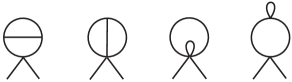
Figure 2: Momentum-independent contribution to the two-point function at the two-loop order.

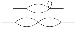
Figure 3: Diagrammatic topologies which can be reduced to the one-loop case.

II SZM identity at one-loop order

II.1 One-loop self-energy

In a theory of scalar fields, all the diagrammatic topologies depicted in the present work would represent the full contribution to a given amplitude. When considering a spinor, vector or tensor theory (like gravity), there may be several components associated with a given topology. As will be clear in what follows, for the purpose of our present analysis, it is not necessary to make explicit which component we are taking into account. All components can be encompassed in the same framework, so that whenever we refer to a given amplitude, we are in fact considering several components.

In this subsection we will consider, as a simple example, the one-loop self-energy. This will illustrate our basic idea and also allow us to introduce the main notation.

There are two basic topologies which contribute to the self-energy at the one-loop order. The first topology, shown in Fig. 1, is independent of the external momentum, and the SZM identity is trivial. The only nontrivial topology which contributes to the one-loop self-energy is shown in Fig. 4.

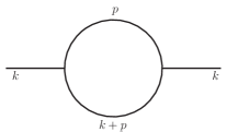
Figure 4: A nontrivial one-loop contribution to the self-energy.

In the static limit ($k_{0}=0$), this amplitude can be written as

$$\Pi_{e}=\oint_{C}\frac{dp_{0}}{2\pi i}\frac{f(p_{0})}{(p_{0}^{2}-x^{2})(p_{0}^{2}-w^{2})},$$ (1)

where $x=|\vec{p}|$ and $w=|\vec{p}+\vec{k}|$. (In this work we will omit the integration over the spacial components of the loop momenta since it is not important for the validity of our arguments; we remark that this makes our results valid in $d$ space-time dimensions.) Here we are using the usual expression for the Matsubara sum in terms of an integral over the contours $C_{1}$ and $C_{2}$ shown in Fig. 5 (a). For the temperature-dependent part, the numerator $f(p_{0})$ reduces to

$$f(p_{0})=N_{p}(p_{0})V(p^{\mu}).$$ (2)

Here $N_{p}(p_{0})$ is the distribution of Fermi-Dirac or Bose-Einstein, depending on the parity of the line $p_{0}$. (In the contour $C_{2}$ it is convenient to make $f(p_{0})\rightarrow-N(-p_{0})V(p^{\mu})$, which is valid for the temperature-dependent contribution.)

The function $V(p^{\mu})$ is model dependent, and it represents some tensor or spinor component. In general, the function $V$ depends on the external four-momentum $k$. However, for the Yang-Mills theory or gravity, the components of $V$ are polynomials, and so, in the high-temperature limit, we can make $k=0$ in $V$ Bellac (1996); Kapusta (1989). For our present purposes, the only relevant momentum dependence of $f$ is the temporal component of the momentum $p_{0}$.

Using the asymptotic behavior of $N_{p}(p_{0})$, we can close the path $C$ at the infinity as we shown in Fig. 5 (b).

$$\begin{array}[]{c}\includegraphics[scale={0.5}]{contorno-a}\\ \\ (a)\\ \includegraphics[scale={0.5}]{contorno-b}\\ \\ (b)\end{array}$$

Figure 5: Integration paths on the complex plane $p_{0}$.

By the residue theorem, we have

$$\Pi_{e} =-\left[\frac{f(x)}{2x(x^{2}-w^{2})}+(x\rightarrow-x)\right.$$

$$+\left.\frac{f(w)}{2w(w^{2}-x^{2})}+(w\rightarrow-w)\right]$$

$$=-\frac{1}{x^{2}-w^{2}}\left[\frac{f(x)}{2x}-\frac{f(w)}{2w}\right.$$

$$+\left.(x,w\rightarrow-x,-w)\right].$$ (3)

In the high-temperature limit, the amplitude will be dominated by the region in which the external momentum is much smaller than the integration momentum, namely the hard thermal loops (HTL) region Bellac (1996); Kapusta (1989). Therefore, we can write $w=x+\epsilon$, where $\epsilon=w-x\ll x$, and perform an expansion around $\epsilon=0$, so that

$$\frac{1}{x^{2}-w^{2}}\left[\frac{f(x)}{2x}-\frac{f(w)}{2w}\right]\simeq\frac{1}{2x}\frac{d}{dx}\frac{f(x)}{2x}.$$ (4)

This yields the following contribution to the high-temperature limit of the static self-energy:

$$\Pi_{e}\simeq-\left[\frac{1}{2x}\frac{d}{dx}\frac{f(x)}{2x}+(x\rightarrow-x)\right].$$ (5)

Let us now consider the other side of the SZM identity, namely the zero-momentum limit. In this case, the self-energy reduces to

$$\Pi_{0}=\oint_{C}\frac{dp_{0}}{2\pi i}\frac{f(p_{0})}{(p_{0}^{2}-x^{2})^{2}}.$$ (6)

Using the residue theorem, we can integrate in $p_{0}$, obtaining

$$\Pi_{0}=-\left[\lim_{p_{0}\rightarrow x}\frac{d}{dp_{0}}\frac{f(p_{0})}{(p_{0}+x)^{2}}+(x\rightarrow-x)\right].$$ (7)

Evaluating the limit, we obtain

$$\lim_{p_{0}\rightarrow x}\frac{d}{dp_{0}}\frac{f(p_{0})}{(p_{0}+x)^{2}}=\frac{1}{4x^{2}}\frac{d}{dx}f(x)-\frac{f(x)}{4x^{3}}$$

$$=\frac{1}{2x}\frac{d}{dx}\frac{f(x)}{2x}.$$ (8)

Therefore, the zero-momentum limit reduces to

$$\Pi_{0}=-\left[\frac{1}{2x}\frac{d}{dx}\frac{f(x)}{2x}+(x\rightarrow-x)\right],$$ (9)

which is identical to the result in Eq. (5). This shows that the contribution of the one-loop nontrivial topology in Fig. 4 satisfies the SZM identity. Taking into account also the trivial contribution in Fig. 1, we conclude that the one-loop self-energy satisfies the SZM identity.

From the explicit expressions for the diagrams shown in Fig. 3 we can see that the SZM identity follows from a similar derivation as above. Indeed, in this type of diagram the loop integrals are independent of each other.

II.2 Iterative procedure for one-loop amplitudes

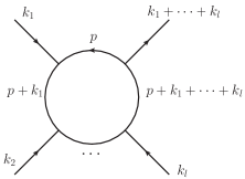
Figure 6: 1PI one-loop amplitude with $l+1$ vertices. It is to be understood that some of the external lines may represent a bundle of lines which intersect on the same vertex.

Let us now consider all possible 1PI one-loop amplitudes with an arbitrary number of external lines. Fig. 6 shows a diagram containing $l+1$ vertices. For a general diagrammatic topology, $k_{i}$ denotes the sum of $n_{i}=1,\,2\,\dots$ individual four-momenta associated with the $n_{i}$ lines intersecting on a ($n_{i}+2$)-point vertex, so that the total number of external lines is given by $\sum_{i}n_{i}\geq l+1$.

In the static limit, when the time component of all external four-momenta vanishes (${k_{0}}_{i}=0$), this amplitude can be written as (recall that we are not concerned with the integrations over the space components of the loop momentum)

$$\mathcal{A}^{l+1}_{e}=\oint_{C}\frac{dp_{0}}{2\pi i}\frac{{\bar{f}}(p_{0})}{(p_{0}^{2}-x^{2})}\prod_{n=1}^{l}\frac{1}{p_{0}^{2}-w_{n}^{2}},$$ (10)

where we have introduced the notation

$$w_{n}=\left|\vec{p}+\vec{k}_{1}+\cdots+\vec{k}_{n}\right|,$$ (11)

and $x=\left|\vec{p}\right|$. At high-temperature, the function ${\bar{f}}(p_{0})$ has similar properties to $f(p_{0})$ in Eq. (2), being the product of the thermal distribution and components of a tensor independent of the external momentum.

Performing the $p_{0}$ integration with the help of the residue theorem, and using the contour depicted in the Fig. 5 (b), we obtain

$$\mathcal{A}^{l+1}_{e} =-\left\{\frac{{\bar{f}}(x)}{2x}\prod_{n=1}^{l}\frac{1}{x^{2}-w_{n}^{2}}\right.$$

$$+\left.\sum_{m=1}^{l}\frac{{\bar{f}}(w_{m})}{2w_{m}(w_{m}^{2}-x^{2})}\prod_{\mathrel{\leavevmode\hbox{\raisebox{2.41112pt}{$\hskip 13.71835pt\raisebox{-4.63551pt}{\makebox[13.71835pt]{\leavevmode\hbox{$\scriptstyle{n\neq m}$}}}\raisebox{1.20552pt}{\makebox[13.71835pt]{\leavevmode\hbox{$\scriptstyle{n=1}$}}}$}}}}^{l}\frac{1}{w_{m}^{2}-w_{n}^{2}}\right\}$$

$$+\{(x,w_{j})\rightarrow(-x,-w_{j})\}\;\;j=1\dots l.$$ (12)

In order to attain the full high-temperature limit of the static amplitude, we now consider an iterative procedure. Our strategy, in order to reach the HTL region, is to perform a step-by-step procedure considering each external momentum $\vec{k}_{i}$ small compared with $\vec{p}$.

Let us first single out the dependence on $w_{1}$, so that Eq. (II.2) can be written as

$$\mathcal{A}^{l+1}_{e} =-\left\{\frac{1}{x^{2}-w_{1}^{2}}\left(\frac{{\bar{f}}(x)}{2x}\prod_{n=2}^{l}\frac{1}{x^{2}-w_{n}^{2}}-\frac{{\bar{f}}(w_{1})}{2w_{1}}\prod_{n=2}^{l}\frac{1}{w_{1}^{2}-w_{n}^{2}}\right)+\sum_{m=2}^{l}\frac{{\bar{f}}(w_{m})}{2w_{m}(w_{m}^{2}-x^{2})(w_{m}^{2}-w_{1}^{2})}\prod_{\mathrel{\leavevmode\hbox{\raisebox{2.41112pt}{$\hskip 13.71835pt\raisebox{-4.63551pt}{\makebox[13.71835pt]{\leavevmode\hbox{$\scriptstyle{n\neq m}$}}}\raisebox{1.20552pt}{\makebox[13.71835pt]{\leavevmode\hbox{$\scriptstyle{n=2}$}}}$}}}}^{l}\frac{1}{w_{m}^{2}-w_{n}^{2}}\right\}$$

$$+\{(x,w_{j})\rightarrow(-x,-w_{j})\}\;\;j=1\dots l$$ (13)

We now consider the external momentum $\vec{k}_{1}$ much smaller than the loop momentum $\vec{p}$, so that, proceeding as in the previous sub-section, we can write $w_{1}=x+\epsilon$ and expand around $\epsilon=0$. This yields

$$\mathcal{A}^{l+1}_{e} \simeq-\left\{\frac{1}{2x}\frac{\partial}{\partial x}\left(\frac{{\bar{f}}(x)}{2x}\prod_{n=2}^{l}\frac{1}{x^{2}-\bar{w}_{n}^{2}}\right)\right.$$

$$+\left.\sum_{m=2}^{l}\frac{{\bar{f}}(\bar{w}_{m})}{2\bar{w}_{m}(\bar{w}_{m}^{2}-x^{2})^{2}}\prod_{\mathrel{\leavevmode\hbox{\raisebox{2.41112pt}{$\hskip 13.71835pt\raisebox{-4.63551pt}{\makebox[13.71835pt]{\leavevmode\hbox{$\scriptstyle{n\neq m}$}}}\raisebox{1.20552pt}{\makebox[13.71835pt]{\leavevmode\hbox{$\scriptstyle{n=2}$}}}$}}}}^{l}\frac{1}{\bar{w}_{m}^{2}-\bar{w}_{n}^{2}}\right\}$$

$$+\{(x,\bar{w}_{j})\rightarrow(-x,-\bar{w}_{j})\}\;\;j=2\dots l,$$ (14)

with the notation

$$\bar{w}_{n}=\left|\vec{p}+\vec{k}_{2}+\cdots+\vec{k}_{n}\right|\;\;n=2\dots l.$$ (15)

Using the residue theorem we can write Eq. (14) as

$$\mathcal{A}^{l+1}_{e} \simeq\frac{1}{2x}\frac{\partial}{\partial x}\oint_{C}\frac{dp_{0}}{2\pi i}\frac{{\bar{f}}(p_{0})}{(p_{0}^{2}-x^{2})}\prod_{n=2}^{l}\frac{1}{p_{0}^{2}-\bar{w}_{n}^{2}}$$

$$=\oint_{C}\frac{dp_{0}}{2\pi i}\frac{{\bar{f}}(p_{0})}{(p_{0}^{2}-x^{2})^{2}}\prod_{n=2}^{l}\frac{1}{p_{0}^{2}-\bar{w}_{n}^{2}}.$$ (16)

On the other hand, if we make $\vec{k}_{1}=0$ in the static amplitude [Eq. (10)], we obtain an amplitude with zero four-momenta ($k_{1}=0$), which is the same as Eq. (16). This special case of the SZM identity is the basis for the inductive reasoning to be employed in what follows. Notice that, in the particular case where $l=1$, Eqs. (10) (with $\vec{k}_{1}=0$) and Eq. (16) explicitly verify the SZM identity for the self-energy, as in the previous section.

In order to complete the inductive reasoning, let us now assume that the amplitude, with $\vec{k}_{1},\,\,\dots,\,\,\vec{k}_{n-1}$ much smaller than the loop momentum $\vec{p}$, can be approximated by

$$\mathcal{A}^{l+1}_{e} \simeq\oint_{C}\frac{dp_{0}}{2\pi i}\frac{{\bar{f}}(p_{0})}{(p_{0}^{2}-x^{2})^{n}}\prod_{i=n}^{l}\frac{1}{p_{0}^{2}-v_{i}^{2}},$$ (17)

where

$$v_{i}=\left|\vec{p}+\vec{k}_{n}+\cdots+\vec{k}_{i}\right|\;\;i=n,\;\;\dots,\;\;l.$$ (18)

Then, starting from Eq. (17), we will prove that, when the momentum $\vec{k}_{n}$ is also much smaller than $\vec{p}$, we obtain Eq. (17) with $n\rightarrow n+1$ [see Eqs. (31) (34)].

Using the residue theorem, the $p_{0}$ integration in Eq. (17) yields

$$\mathcal{A}^{l+1}_{e} \simeq-\left\{\lim_{p_{0}\rightarrow x}\frac{1}{(n-1)!}\left(\frac{\partial}{\partial p_{0}}\right)^{n-1}\frac{\bar{f}(p_{0})}{(p_{0}+x)^{n}}\prod_{i=n}^{l}\frac{1}{p_{0}^{2}-v_{i}^{2}}+\sum_{j=n}^{l}\frac{\bar{f}(v_{j})}{2v_{j}(v_{j}^{2}-x^{2})^{n}}\prod_{\mathrel{\leavevmode\hbox{\raisebox{2.41112pt}{$\hskip 11.24033pt\raisebox{-4.63551pt}{\makebox[11.24033pt]{\leavevmode\hbox{$\scriptstyle{i\neq j}$}}}\raisebox{1.20552pt}{\makebox[11.24033pt]{\leavevmode\hbox{$\scriptstyle{i=n}$}}}$}}}}^{l}\frac{1}{v_{j}^{2}-v_{i}^{2}}\right\}$$

$$+\{(x,v_{m})\rightarrow(-x,-v_{m})\}\;\;m=2\dots l,$$

$$=-\left\{\lim_{p_{0}\rightarrow x}\frac{1}{(n-1)!}\left(\frac{\partial}{\partial p_{0}}\right)^{n-1}\frac{\bar{f}(p_{0})}{(p_{0}+x)^{n}(p_{0}^{2}-v_{n}^{2})}\prod_{i=n+1}^{l}\frac{1}{p_{0}^{2}-v_{i}^{2}}+\frac{\bar{f}(v_{n})}{2v_{n}(v_{n}^{2}-x^{2})^{n}}\prod_{i=n+1}^{l}\frac{1}{v_{n}^{2}-v_{i}^{2}}\right.$$

$$+\left.\sum_{j=n+1}^{l}\frac{\bar{f}(v_{j})}{2v_{j}(v_{j}^{2}-x^{2})^{n}(v_{j}^{2}-v_{n}^{2})}\prod_{\mathrel{\leavevmode\hbox{\raisebox{2.41112pt}{$\hskip 17.50143pt\raisebox{-4.63551pt}{\makebox[17.50143pt]{\leavevmode\hbox{$\scriptstyle{i\neq j}$}}}\raisebox{1.61385pt}{\makebox[17.50143pt]{\leavevmode\hbox{$\scriptstyle{i=n+1}$}}}$}}}}^{l}\frac{1}{v_{j}^{2}-v_{i}^{2}}\right\}+\{(x,v_{m})\rightarrow(-x,-v_{m})\}\;\;m=n,\;\;\dots,\;\;l.$$ (19)

The first term in Eq. (19) can be written as

$$T_{1} =\lim_{p_{0}\rightarrow x}\frac{1}{(n-1)!}\left(\frac{\partial}{\partial p_{0}}\right)^{n-1}\frac{h(p_{0})}{(p_{0}+x)^{n}(p_{0}^{2}-v_{n}^{2})}$$

$$=\lim_{p_{0}\rightarrow x}\frac{1}{(n-1)!}\left(\frac{\partial}{\partial p_{0}}\right)^{n-1}$$

$$\times\frac{h(p_{0})}{(p_{0}+x)^{n}(p_{0}+v_{n})(p_{0}-v_{n})},$$ (20)

where we have introduced

$$h(p_{0})=\bar{f}(p_{0})\prod_{i=n+1}^{l}\frac{1}{p_{0}^{2}-v_{i}^{2}}.$$ (21)

Using the Leibniz rule, we have an analogy with the binomial formula, such that

$$\left(\frac{\partial}{\partial p_{0}}\right)^{n-1}[A(p_{0})B(p_{0})]=\sum_{t=0}^{n-1}\frac{(n-1)!}{t!(n-1-t)!}\left[\left(\frac{\partial}{\partial p_{0}}\right)^{t}A(p_{0})\right]\left[\left(\frac{\partial}{\partial p_{0}}\right)^{n-1-t}B(p_{0})\right],$$ (22)

so that Eq. (20) acquires the form

$$T_{1} =\sum_{t=0}^{n-1}\frac{1}{t!(n-1-t)!}\lim_{p_{0}\rightarrow x}\left[\left(\frac{\partial}{\partial p_{0}}\right)^{n-1-t}\frac{1}{p_{0}-v_{n}}\right]\left[\left(\frac{\partial}{\partial p_{0}}\right)^{t}\frac{h(p_{0})}{(p_{0}+x)^{n}(p_{0}+v_{n})}\right].$$ (23)

Evaluating the derivative yields

$$T_{1} =\sum_{t=0}^{n-1}\frac{1}{t!(n-1-t)!}\lim_{p_{0}\rightarrow x}\left[\frac{(-1)^{n-t-1}(n-t-1)!}{(p_{0}-v_{n})^{n-t}}\right]\left[\left(\frac{\partial}{\partial p_{0}}\right)^{t}\frac{h(p_{0})}{(p_{0}+x)^{n}(p_{0}+v_{n})}\right]$$

$$=\sum_{t=0}^{n-1}\frac{1}{t!}\lim_{p_{0}\rightarrow x}\left[\frac{-1}{(v_{n}-p_{0})^{n-t}}\right]\left[\left(\frac{\partial}{\partial p_{0}}\right)^{t}\frac{h(p_{0})}{(p_{0}+x)^{n}(p_{0}+v_{n})}\right]$$

$$=\sum_{t=0}^{n-1}\frac{1}{t!}\frac{-1}{(v_{n}-x)^{n-t}}\lim_{p_{0}\rightarrow x}\left(\frac{\partial}{\partial p_{0}}\right)^{t}\frac{h(p_{0})}{(p_{0}+x)^{n}(p_{0}+v_{n})}.$$ (24)

We now introduce the high-temperature limit, when momentum $\vec{k}_{n}$ is much smaller than the integration momentum $\vec{p}$, so that $v_{n}=x+\epsilon$. Then, the dominant term in Eq. (II.2) is

$$T_{1} \simeq-\sum_{t=0}^{n-1}\frac{1}{t!(v_{n}-x)^{n-t}}\lim_{p_{0}\rightarrow x}\left(\frac{\partial}{\partial p_{0}}\right)^{t}\frac{h(p_{0})}{(p_{0}+x)^{n+1}}.$$ (25)

Similarly, using Eq. (21), the second term in Eq. (19) can be written as

$$T_{2}=\frac{1}{(v_{n}-x)^{n}}\frac{h(v_{n})}{2v_{n}(v_{n}+x)^{n}}.$$ (26)

In the high-temperature limit, we can make the approximation

$$T_{2}\simeq\frac{1}{(v_{n}-x)^{n}}\frac{h(v_{n})}{(v_{n}+x)^{n+1}}$$ (27)

and perform the Taylor expansion, yielding

$$T_{2}\simeq\frac{1}{(v_{n}-x)^{n}}\sum_{t=0}^{\infty}\frac{(v_{n}-x)^{t}}{t!}\lim_{v_{n}\rightarrow x}\left(\frac{\partial}{\partial v_{n}}\right)^{t}\frac{h(v_{n})}{(v_{n}+x)^{n+1}},$$ (28)

which can be rewritten as

$$T_{2}\simeq\sum_{t=0}^{\infty}\frac{1}{t!(v_{n}-x)^{n-t}}\lim_{p_{0}\rightarrow x}\left(\frac{\partial}{\partial p_{0}}\right)^{t}\frac{h(p_{0})}{(p_{0}+x)^{n+1}}.$$ (29)

Combining Eqs. (25) and (29) and neglecting all the subleading contributions in the high-temperature limit, we obtain

$$T_{1}+T_{2}\simeq\frac{1}{n!}\lim_{p_{0}\rightarrow x}\left(\frac{\partial}{\partial p_{0}}\right)^{n}\frac{h(p_{0})}{(p_{0}+x)^{n+1}}$$

$$\simeq\frac{1}{n!}\lim_{p_{0}\rightarrow x}\left(\frac{\partial}{\partial p_{0}}\right)^{n}\frac{\bar{f}(p_{0})}{(p_{0}+x)^{n+1}}\prod_{{i=n+1}}^{l}\frac{1}{p_{0}^{2}-\bar{v}_{i}^{2}},$$ (30)

where

$$\bar{v}_{i}=\left|\vec{p}+\vec{k}_{n+1}+\cdots+\vec{k}_{i}\right|\,\,,i=n+1,\,\,\cdots,\,\,l.$$ (31)

The last term in Eq. (19) has the following high-temperature limit

$$T_{3}\simeq\sum_{j=n+1}^{l}\frac{\bar{f}(\bar{v}_{j})}{2\bar{v}_{j}(\bar{v}_{j}^{2}-x^{2})^{n+1}}\prod_{\mathrel{\leavevmode\hbox{\raisebox{2.41112pt}{$\hskip 17.50143pt\raisebox{-4.63551pt}{\makebox[17.50143pt]{\leavevmode\hbox{$\scriptstyle{i\neq j}$}}}\raisebox{1.61385pt}{\makebox[17.50143pt]{\leavevmode\hbox{$\scriptstyle{i=n+1}$}}}$}}}}^{l}\frac{1}{\bar{v}_{j}^{2}-\bar{v}_{i}^{2}}.$$ (32)

Combining Eqs. (II.2) and (32), we obtain

$$\mathcal{A}^{l+1}_{e} \simeq-\left\{\frac{1}{n!}\lim_{p_{0}\rightarrow x}\left(\frac{\partial}{\partial p_{0}}\right)^{n}\frac{\bar{f}(p_{0})}{(p_{0}+x)^{n+1}}\prod_{{i=n+1}}^{l}\frac{1}{p_{0}^{2}-\bar{v}_{i}^{2}}+\sum_{j=n+1}^{l}\frac{\bar{f}(\bar{v}_{j})}{2\bar{v}_{j}(\bar{v}_{j}^{2}-x^{2})^{n+1}}\prod_{\mathrel{\leavevmode\hbox{\raisebox{2.41112pt}{$\hskip 17.50143pt\raisebox{-4.63551pt}{\makebox[17.50143pt]{\leavevmode\hbox{$\scriptstyle{i\neq j}$}}}\raisebox{1.61385pt}{\makebox[17.50143pt]{\leavevmode\hbox{$\scriptstyle{i=n+1}$}}}$}}}}^{l}\frac{1}{\bar{v}_{j}^{2}-\bar{v}_{i}^{2}}\right\}$$

$$+\{(x,\bar{v}_{m})\rightarrow(-x,-\bar{v}_{m})\}\;\;m=n+1,\;\;\dots,\;\;l.$$ (33)

Finally, using the residue theorem yields

$$\mathcal{A}^{l+1}_{e} \simeq\oint_{C}\frac{dp_{0}}{2\pi i}\frac{{\bar{f}}(p_{0})}{(p_{0}^{2}-x^{2})^{n+1}}\prod_{i=n+1}^{l}\frac{1}{p_{0}^{2}-\bar{v}_{i}^{2}}.$$ (34)

This completes the inductive reasoning for all one-loop HTL amplitudes.

As a direct consequence of the previous proof, we now can write

$$\mathcal{A}^{l+1}_{e}\simeq\oint_{C}\frac{dp_{0}}{2\pi i}\frac{\bar{f}(p_{0})}{(p_{0}^{2}-x^{2})^{l+1}}=\mathcal{A}^{l+1}_{0},$$ (35)

which generalizes the result obtained in Ref. Frenkel et al. (2009). Then, from this general SZM identity, we can immediately write the result for a general 1PI one-loop static amplitude, in the HTL approximation, as follows:

$$\mathcal{A}^{l+1}_{e} \simeq\frac{1}{l!}\left(\frac{1}{2x}\frac{\partial}{\partial x}\right)^{l}\oint_{C}\frac{dp_{0}}{2\pi i}\frac{\bar{f}(p_{0})}{p_{0}^{2}-x^{2}}$$

$$=\frac{1}{l!}\left(\frac{1}{2x}\frac{\partial}{\partial x}\right)^{l}\frac{\bar{f}(x)}{2x}+(x\rightarrow-x).$$ (36)

This equation gives the general expression for 1PI amplitudes in the high-temperature static limit, after we explicitly consider some field theory model and integrate over the space components of the loop momentum. It is easy to verify that in $d$ space-time dimensions, the power of the temperature will be $[V]+d-2l-2$ (where $[V]$ denotes the mass dimension of the tensor structure). In the case of scalar ($[V]=0$) and vector gauge theories the leading high-temperature behavior will be $T^{d-4}$ and $T^{d-2}$, respectively, while for gravity, the 1PI amplitudes contribute to all orders being proportional to $T^{d}$.

III Self-energy at two-loop order

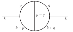
Figure 7: First contribution for two-loop self energy

In this section we will consider the two-loop contributions to the self-energy. Now we have to consider all types of nontrivial topologies which, unlike the ones shown in Figs. 2 and 3, are dependent on the external momentum and cannot be reduced to the one-loop case. There are five such topologies. Here we will present the details of two of them, which are representative of the technicalities and illustrate the main aspects of this analysis. The other three topologies will be considered in the Appendix.

III.1 First topology

Let us first consider the contribution shown in Fig. 7. In the static limit, this amplitude can be written as

$$\Pi_{e}^{A}=\oint_{C}\frac{dp_{0}}{2\pi i}\oint_{C}\frac{dq_{0}}{2\pi i}\frac{f^{A}(p_{0},q_{0})}{(p_{0}^{2}-x^{2})(p_{0}^{2}-w^{2})[(p_{0}-q_{0})^{2}-z^{2}](q_{0}^{2}-y^{2})(q_{0}^{2}-v^{2})},$$ (37)

where $x=|\vec{p}|$, $y=|\vec{q}|$, $w=|\vec{p}+\vec{k}|$, $v=|\vec{q}+\vec{k}|$ and $z=|\vec{p}-\vec{q}|$. The hard thermal loop region, which yields leading high-temperature contributions, comes from the terms containing the product of two thermal distributions so that the function $f^{A}(p_{0},q_{0})$ has the following form (there are indications that these terms may be the only ones which survive in the high-temperature limit Mottola:2009mi )

$$f^{A}(p_{0},q_{0})=N_{p}(p_{0})N_{q}(q_{0})V(p^{\mu},q^{\nu}),$$ (38)

and the same high-temperature considerations we have made for $f(p_{0})$ in Sec.  II.1 also holds for $f^{A}(p_{0},q_{0})$, so that it does not depend on the external momentum.

Using the residue theorem to perform the $p_{0}$ integration yields

$$\Pi_{e}^{A} =-\oint_{C}\frac{dq_{0}}{2\pi i}\left\{\frac{f^{A}(x,q_{0})}{2x(x^{2}-w^{2})[(x-q_{0})^{2}-z^{2}](q_{0}^{2}-y^{2})(q_{0}^{2}-v^{2})}\right.$$

$$+\left.\frac{f^{A}(w,q_{0})}{2w(w^{2}-x^{2})[(w-q_{0})^{2}-z^{2}](q_{0}^{2}-y^{2})(q_{0}^{2}-v^{2})}\right.$$

$$+\left.\frac{f^{A}(q_{0}+z,q_{0})}{2z[(q_{0}+z)^{2}-x^{2}][(q_{0}+z)^{2}-w^{2}](q_{0}^{2}-y^{2})(q_{0}^{2}-v^{2})}\right\}+\{(x,w,z)\rightarrow(-x,-w,-z)\}.$$ (39)

Similarly, the $q_{0}$ integral produces

$$\Pi_{e}^{A} =\left\{\left[\frac{f^{A}(x,x+z)}{4zx(x^{2}-w^{2})[(x+z)^{2}-y^{2}][(x+z)^{2}-v^{2}]}+\frac{f^{A}(w,w+z)}{4zw(w^{2}-x^{2})[(w+z)^{2}-y^{2}][(w+z)^{2}-v^{2}]}\right.\right.$$

$$+\left.\left.(z\rightarrow-z)\right]+\left[\frac{f^{A}(x,y)}{4xy(x^{2}-w^{2})[(x-y)^{2}-z^{2}](y^{2}-v^{2})}+\frac{f^{A}(w,y)}{4wy(w^{2}-x^{2})[(w-y)^{2}-z^{2}](y^{2}-v^{2})}\right.\right.$$

$$+\left.\left.\frac{f^{A}(y+z,y)}{4zy[(y+z)^{2}-x^{2}][(y+z)^{2}-w^{2}](y^{2}-v^{2})}+(y\rightarrow-y)\right]\right.$$

$$+\left.\left[\frac{f^{A}(x,v)}{4xv(x^{2}-w^{2})[(x-v)^{2}-z^{2}](v^{2}-y^{2})}+\frac{f^{A}(w,v)}{4wv(w^{2}-x^{2})[(w-v)^{2}-z^{2}](v^{2}-y^{2})}\right.\right.$$

$$+\left.\left.\frac{f^{A}(v+z,v)}{4zv[(v+z)^{2}-x^{2}][(v+z)^{2}-w^{2}](v^{2}-y^{2})}+(v\rightarrow-v)\right]+\left[\frac{f^{A}(x,x-z)}{4zx(x^{2}-w^{2})[(x-z)^{2}-y^{2}][(x-z)^{2}-v^{2}]}\right.\right.$$

$$+\left.\left.(x\rightarrow-x)\right]+\left[\frac{f^{A}(w,w-z)}{4zw(w^{2}-x^{2})[(w-z)^{2}-y^{2}][(w-z)^{2}-v^{2}]}+(w\rightarrow-w)\right]\right\}$$

$$+\left\{[(x,w,z)\rightarrow(-x,-w,-z)]\right\}.$$ (40)

The HTL region is now characterized by $q\gg k$ and $p\gg k$, so that we can write $w=x+\epsilon$ and $v=y+\delta$, with $\epsilon=w-x\ll x$ and $\delta=v-y\ll y$, and a series expansion can be performed around $\epsilon=0$ and $\delta=0$. In this way, all the terms in Eq. (III.1) can be dealt with using the following relations:

$$\frac{1}{x^{2}-w^{2}}\left[\frac{f^{A}(x,x+z)}{4zx[(x+z)^{2}-y^{2}][(x+z)^{2}-v^{2}]}\right.$$

$$-\left.\frac{f^{A}(w,w+z)}{4zw[(w+z)^{2}-y^{2}][(w+z)^{2}-v^{2}]}\right]\simeq$$

$$\simeq\frac{1}{2x}\frac{\partial}{\partial x}\left[\frac{f^{A}(x,x+z)}{4zx[(x+z)^{2}-y^{2}]^{2}}\right],$$ (41)

$$\frac{1}{y^{2}-v^{2}}\left[\frac{f^{A}(y+z,y)}{4zy[(y+z)^{2}-x^{2}][(y+z)^{2}-w^{2}]}\right.$$

$$-\left.\frac{f^{A}(v+z,v)}{4zv[(v+z)^{2}-x^{2}][(v+z)^{2}-w^{2}]}\right]$$

$$\simeq\frac{1}{2y}\frac{\partial}{\partial y}\left[\frac{f^{A}(y+z,y)}{4zy[(y+z)^{2}-x^{2}]^{2}}\right],$$ (42)

$$\frac{1}{x^{2}-w^{2}}\left[\frac{f^{A}(x,x-z)}{4zx[(x-z)^{2}-y^{2}][(x-z)^{2}-v^{2}]}\right.$$

$$-\left.\frac{f^{A}(w,w-z)}{4zw[(w-z)^{2}-y^{2}][(w-z)^{2}-v^{2}]}\right]$$

$$\simeq\frac{1}{2x}\frac{\partial}{\partial x}\left[\frac{f^{A}(x,x-z)}{4zx[(x-z)^{2}-y^{2}]^{2}}\right],$$ (43)

$$\frac{1}{x^{2}-w^{2}}\frac{1}{y^{2}-v^{2}}\left[g(x,y)-g(w,y)-g(x,v)+g(w,v)\right]$$

$$\simeq\frac{1}{2x}\frac{\partial}{\partial x}\frac{1}{y^{2}-v^{2}}\left[g(x,y)-g(x,v)\right]$$

$$\simeq\frac{1}{4xy}\frac{\partial^{2}}{\partial x\partial y}g(x,y),$$ (44)

with

$$g(x,y)=\frac{f^{A}(x,y)}{4xy[(x-y)^{2}-z^{2}]}.$$ (45)

Substituting these results back into Eq. (III.1), we obtain the following static hard thermal loop approximation:

$$\Pi_{e}^{A} \simeq\left\{\frac{1}{2x}\frac{\partial}{\partial x}\left[\frac{f^{A}(x,x+z)}{4zx[(x+z)^{2}-y^{2}]^{2}}\right]+[z\rightarrow-z]\right.$$

$$+\left.\frac{1}{2x}\frac{\partial}{\partial x}\left[\frac{f^{A}(x,x-z)}{4zx[(x-z)^{2}-y^{2}]^{2}}\right]+[x\rightarrow-x]\right.$$

$$+\left.\frac{1}{2y}\frac{\partial}{\partial y}\left[\frac{f^{A}(y+z,y)}{4zy[(y+z)^{2}-x^{2}]^{2}}\right]+[y\rightarrow-y]\right.$$

$$+\left.\frac{1}{4xy}\frac{\partial^{2}}{\partial x\partial y}\frac{f^{A}(x,y)}{4xy[(x-y)^{2}-z^{2}]}+[y\rightarrow-y]\right\}$$

$$+\{(x,z)\rightarrow(-x,-z)\}.$$ (46)

Let us now consider the zero-momentum limit. In this case Eq. (37) reduces to

$$\Pi_{0}^{A}=\oint_{C}\frac{dp_{0}}{2\pi i}\oint_{C}\frac{dq_{0}}{2\pi i}\frac{f^{A}(p_{0},q_{0})}{(p_{0}^{2}-x^{2})^{2}[(p_{0}-q_{0})^{2}-z^{2}](q_{0}^{2}-y^{2})^{2}}.$$ (47)

Using the residue theorem, the $p_{0}$ integration yields

$$\Pi_{0}^{A} =-\oint_{C}\frac{dq_{0}}{2\pi i}\left\{\frac{f^{A}(q_{0}+z,q_{0})}{2z[(q_{0}+z)^{2}-x^{2}]^{2}(q_{0}^{2}-y^{2})^{2}}+(z\rightarrow-z)+\lim_{p_{0}\rightarrow x}\frac{\partial}{\partial p_{0}}\frac{f^{A}(p_{0},q_{0})}{(p_{0}+x)^{2}[(p_{0}-q_{0})^{2}-z^{2}](q_{0}^{2}-y^{2})^{2}}\right.$$

$$+\left.(x\rightarrow-x)\right\}$$

$$=-\oint_{C}\frac{dq_{0}}{2\pi i}\left\{\left[\frac{f^{A}(q_{0}+z,q_{0})}{2z[(q_{0}+z)^{2}-x^{2}]^{2}(q_{0}^{2}-y^{2})^{2}}+\frac{1}{2x}\frac{\partial}{\partial x}\frac{f^{A}(x,q_{0})}{2x[(x-q_{0})^{2}-z^{2}](q_{0}^{2}-y^{2})^{2}}\right]\right.$$

$$+\left.[(x,z)\rightarrow(-x,-z)]\right\}.$$ (48)

Similarly, the $q_{0}$ integral produces

$$\Pi_{0}^{A} =\left\{\lim_{q_{0}\rightarrow x-z}\frac{\partial}{\partial q_{0}}\frac{f^{A}(q_{0}+z,q_{0})}{2z(q_{0}+z+x)^{2}(q_{0}^{2}-y^{2})^{2}}+(x\rightarrow-x)+\lim_{q_{0}\rightarrow y}\frac{\partial}{\partial q_{0}}\frac{f^{A}(q_{0}+z,q_{0})}{2z[(q_{0}+z)^{2}-x^{2}]^{2}(q_{0}+y)^{2}}+(y\rightarrow-y)\right.$$

$$+\left.\frac{1}{2x}\frac{\partial}{\partial x}\lim_{q_{0}\rightarrow y}\frac{\partial}{\partial q_{0}}\frac{f^{A}(x,q_{0})}{2x[(x-q_{0})^{2}-z^{2}](q_{0}+y)^{2}}+(y\rightarrow-y)+\frac{1}{2x}\frac{\partial}{\partial x}\frac{f^{A}(x,x+z)}{4xz[(x+z)^{2}-y^{2}]^{2}}+(z\rightarrow-z)\right\}$$

$$+\{(x,z)\rightarrow(-x,-z)\}$$

$$=\left\{\frac{1}{2x}\frac{\partial}{\partial x}\frac{f^{A}(x,x-z)}{4zx[(x-z)^{2}-y^{2}]^{2}}+(x\rightarrow-x)+\frac{1}{2y}\frac{\partial}{\partial y}\frac{f^{A}(y+z,y)}{4zy[(y+z)^{2}-x^{2}]^{2}}+(y\rightarrow-y)\right.$$

$$+\left.\frac{1}{4xy}\frac{\partial^{2}}{\partial x\partial y}\frac{f^{A}(x,y)}{4xy[(x-y)^{2}-z^{2}]}+(y\rightarrow-y)+\frac{1}{2x}\frac{\partial}{\partial x}\frac{f^{A}(x,x+z)}{4xz[(x+z)^{2}-y^{2}]^{2}}+(z\rightarrow-z)\right\}$$

$$+\{(x,z)\rightarrow(-x,-z)\},$$ (49)

which is the same as the static limit [(46)]. This concludes the verification of the SZM identity for the amplitude shown in Fig. 7. It is remarkable that this identity holds even before performing the integrations over $\vec{p}$ and $\vec{q}$.

III.2 Second topology

The topology shown in Fig. 8 has the following form in the static limit:

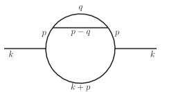
Figure 8: Second topology for two-loop self-energy

$$\Pi_{e}^{B}=\oint_{C}\frac{dp_{0}}{2\pi i}\oint_{C}\frac{dq_{0}}{2\pi i}\frac{f^{B}(p_{0},q_{0})}{(p_{0}^{2}-x^{2})^{2}(p_{0}^{2}-w^{2})[(p_{0}-q_{0})^{2}-z^{2}](q_{0}^{2}-y^{2})}.$$ (50)

In this case we introduce the quantities $x=\left|\vec{p}\right|$, $y=\left|\vec{q}\right|$, $w=|\vec{p}+\vec{k}|$ and $z=\left|\vec{p}-\vec{q}\right|$. In the high-temperature limit, the numerator $f^{B}$ has the same form as $f^{A}$ in Eq. (38). The integrations over $p_{0}$ and $q_{0}$ can be evaluated, as in the previous case, using the residue theorem, yielding

$$\Pi_{e}^{B} =\left\{\left[\frac{1}{2x}\frac{\partial}{\partial x}\frac{f^{B}(x,x-z)}{4xz(x^{2}-w^{2})[(x-z)^{2}-y^{2}]}+(x\rightarrow-x)\right]+\left[\frac{f^{B}(w,w+z)}{4zw(w^{2}-x^{2})^{2}[(w+z)^{2}-y^{2}]}\right.\right.$$

$$+\left.\frac{1}{2x}\frac{\partial}{\partial x}\frac{f^{B}(x,x+z)}{4xz(x^{2}-w^{2})[(x+z)^{2}-y^{2}]}+(z\rightarrow-z)\right]+\left[\frac{f^{B}(w,w-z)}{4zw(w^{2}-x^{2})^{2}[(w-z)^{2}-y^{2}]}+(w\rightarrow-w)\right]$$

$$+\left[\frac{f^{B}(y+z,y)}{4zy[(y+z)^{2}-x^{2}]^{2}[(y+z)^{2}-w^{2}]}+\frac{f^{B}(w,y)}{4wy(w^{2}-x^{2})^{2}[(w-y)^{2}-z^{2}]}\right.$$

$$+\left.\left.\frac{1}{2x}\frac{\partial}{\partial x}\frac{f^{B}(x,y)}{4yx(x^{2}-w^{2})[(x-y)^{2}-z^{2}]}+(y\rightarrow-y)\right]\right\}+\{(x,w,z)\rightarrow(-x,-w,-z)\},$$ (51)

where the derivative terms come from doubles poles. In the HTL region we set $w=x+\epsilon$, with $\epsilon\ll x$. Using relations like

$$\frac{g(w)}{(w^{2}-x^{2})^{2}}+\frac{1}{2x}\frac{\partial}{\partial x}\frac{g(x)}{x^{2}-w^{2}}\simeq\frac{g(x)}{(w^{2}-x^{2})^{2}}+\frac{1}{(w+x)(w^{2}-x^{2})}\frac{\partial}{\partial x}g(x)$$

$$+\frac{1}{2(w+x)^{2}}\frac{\partial^{2}}{\partial x^{2}}g(x)-\frac{1}{(x^{2}-w^{2})^{2}}g(x)+\frac{1}{2x(x^{2}-w^{2})}\frac{\partial}{\partial x}g(x)$$

$$\simeq-\frac{1}{8x^{3}}\frac{\partial}{\partial x}g(x)+\frac{1}{8x^{2}}\frac{\partial^{2}}{\partial x^{2}}g(x),$$ (52)

we obtain from (III.2)

$$\Pi_{e}^{B} \simeq\left\{\left[\left(\frac{1}{8x^{2}}\frac{\partial^{2}}{\partial x^{2}}-\frac{1}{8x^{3}}\frac{\partial}{\partial x}\right)\frac{f^{B}(x,x-z)}{4xz[(x-z)^{2}-y^{2}]}+(x\rightarrow-x)\right]+\left[\left(\frac{1}{8x^{2}}\frac{\partial^{2}}{\partial x^{2}}-\frac{1}{8x^{3}}\frac{\partial}{\partial x}\right)\frac{f^{B}(x,x+z)}{4xz[(x+z)^{2}-y^{2}]}\right.\right.$$

$$+\left.\left.(z\rightarrow-z)\right]+\left[\left(\frac{1}{8x^{2}}\frac{\partial^{2}}{\partial x^{2}}-\frac{1}{8x^{3}}\frac{\partial}{\partial x}\right)\frac{f^{B}(x,y)}{4yx[(x-y)^{2}-z^{2}]}+\frac{f^{B}(y+z,y)}{4zy[(y+z)^{2}-x^{2}]^{3}}+(y\rightarrow-y)\right]\right\}$$

$$+\{(x,z)\rightarrow(-x,-z)\}.$$ (53)

It is also convenient to employ the identity

$$\left(\frac{1}{8x^{2}}\frac{\partial^{2}}{\partial x^{2}}-\frac{1}{8x^{3}}\frac{\partial}{\partial x}\right)\frac{h(x)}{x}=\left(\frac{3}{8x^{5}}-\frac{3}{8x^{4}}\frac{\partial}{\partial x}+\frac{1}{8x^{3}}\frac{\partial^{2}}{\partial x^{2}}\right)h(x),$$ (54)

so that the amplitude takes the final form

$$\Pi_{e}^{B} \simeq\left\{\left[\left(\frac{3}{8x^{5}}-\frac{3}{8x^{4}}\frac{\partial}{\partial x}+\frac{1}{8x^{3}}\frac{\partial^{2}}{\partial x^{2}}\right)\frac{f^{B}(x,x-z)}{4z[(x-z)^{2}-y^{2}]}+(x\rightarrow-x)\right]\right.$$

$$+\left.\left[\left(\frac{3}{8x^{5}}-\frac{3}{8x^{4}}\frac{\partial}{\partial x}+\frac{1}{8x^{3}}\frac{\partial^{2}}{\partial x^{2}}\right)\frac{f^{B}(x,x+z)}{4z[(x+z)^{2}-y^{2}]}+(z\rightarrow-z)\right]\right.$$

$$+\left.\left[\left(\frac{3}{8x^{5}}-\frac{3}{8x^{4}}\frac{\partial}{\partial x}+\frac{1}{8x^{3}}\frac{\partial^{2}}{\partial x^{2}}\right)\frac{f^{B}(x,y)}{4y[(x-y)^{2}-z^{2}]}+\frac{f^{B}(y+z,y)}{4zy[(y+z)^{2}-x^{2}]^{3}}+(y\rightarrow-y)\right]\right\}$$

$$+\{(x,z)\rightarrow(-x,-z)\}.$$ (55)

Let us now consider the zero-momentum limit. In this case, the amplitude shown in Fig. 8 reduces to

$$\Pi_{0}^{B}=\oint_{C}\frac{dp_{0}}{2\pi i}\oint_{C}\frac{dq_{0}}{2\pi i}\frac{f^{B}(p_{0},q_{0})}{(p_{0}^{2}-x^{2})^{3}[(p_{0}-q_{0})^{2}-z^{2}](q_{0}^{2}-y^{2})}.$$ (56)

Integrating in $p_{0}$,

$$\Pi_{0}^{B} =-\oint_{C}\frac{dq_{0}}{2\pi i}\left\{\frac{f^{B}(q_{0}+z,q_{0})}{2z[(q_{0}+z)^{2}-x^{2}]^{3}(q_{0}^{2}-y^{2})}+(z\rightarrow-z)\right.$$

$$+\left.\frac{1}{2}\lim_{p_{0}\rightarrow x}\frac{\partial^{2}}{\partial p_{0}^{2}}\frac{f^{B}(p_{0},q_{0})}{(p_{0}+x)^{3}[(p_{0}-q_{0})^{2}-z^{2}](q_{0}^{2}-y^{2})}+(x\rightarrow-x)\right\}$$ (57)

and computing the limit, yields

$$\Pi_{0}^{B} =\oint_{C}\frac{dq_{0}}{2\pi i}\left\{\left[\frac{f^{B}(q_{0}+z,q_{0})}{2z[(q_{0}+z)^{2}-x^{2}]^{3}(q_{0}^{2}-y^{2})}+\left(\frac{3}{16x^{5}}-\frac{3}{16x^{4}}\frac{\partial}{\partial x}+\frac{1}{16x^{3}}\frac{\partial^{2}}{\partial x^{2}}\right)\frac{f^{B}(x,q_{0})}{[(x-q_{0})^{2}-z^{2}](q_{0}^{2}-y^{2})}\right]\right.$$

$$+\{(x,z)\rightarrow(-x,-z)\}.$$ (58)

Finally, integrating in $q_{0}$, we obtain

$$\Pi_{0}^{B} =\left\{\left[\frac{1}{2}\lim_{q_{0}\rightarrow x-z}\frac{\partial^{2}}{\partial q_{0}^{2}}\frac{f^{B}(q_{0}+z,q_{0})}{2z(q_{0}+z+x)^{3}(q_{0}^{2}-y^{2})}+(x\rightarrow-x)\right]+\left[\frac{f^{B}(y+z,y)}{4zy[(y+z)^{2}-x^{2}]^{3}}+(y\rightarrow-y)\right]\right.$$

$$+\left[\left(\frac{3}{16x^{5}}-\frac{3}{16x^{4}}\frac{\partial}{\partial x}+\frac{1}{16x^{3}}\frac{\partial^{2}}{\partial x^{2}}\right)\frac{f^{B}(x,y)}{2y[(x-y)^{2}-z^{2}]}+(y\rightarrow-y)\right]$$

$$+\left.\left[\left(\frac{3}{16x^{5}}-\frac{3}{16x^{4}}\frac{\partial}{\partial x}+\frac{1}{16x^{3}}\frac{\partial^{2}}{\partial x^{2}}\right)\frac{f^{B}(x,x+z)}{2z[(x+z)^{2}-y^{2}]}+(z\rightarrow-z)\right]\right\}+\{(x,z)\rightarrow(-x,-z)\}$$

$$=\left\{\left[\left(\frac{3}{16x^{5}}-\frac{3}{16x^{4}}\frac{\partial}{\partial x}+\frac{1}{16x^{3}}\frac{\partial^{2}}{\partial x^{2}}\right)\frac{f^{B}(x,x-z)}{2z[(x-z)^{2}-y^{2}]}+(x\rightarrow-x)\right]+\left[\frac{f^{B}(y+z,y)}{4zy[(y+z)^{2}-x^{2}]^{3}}+(y\rightarrow-y)\right]\right.$$

$$+\left[\left(\frac{3}{16x^{5}}-\frac{3}{16x^{4}}\frac{\partial}{\partial x}+\frac{1}{16x^{3}}\frac{\partial^{2}}{\partial x^{2}}\right)\frac{f^{B}(x,y)}{2y[(x-y)^{2}-z^{2}]}+(y\rightarrow-y)\right]$$

$$+\left.\left[\left(\frac{3}{16x^{5}}-\frac{3}{16x^{4}}\frac{\partial}{\partial x}+\frac{1}{16x^{3}}\frac{\partial^{2}}{\partial x^{2}}\right)\frac{f^{B}(x,x+z)}{2z[(x+z)^{2}-y^{2}]}+(z\rightarrow-z)\right]\right\}+\{(x,z)\rightarrow(-x,-z)\},$$ (59)

which is identical to the static-limit result in Eq. (55), in agreement with the SZM identity.

IV Discussion

The results presented in this work may be useful in physical scenarios where there are static external fields and the temperature is high. An important example would arise in the calculation of effective actions in static backgrounds. Indeed, in the configuration space, the SZM identity implies that one may compute the static effective action using a much simpler space-time independent background field configuration. For instance in Ref. Brandt and Siqueira (2012) we have shown that the effective action of static gravitational fields can be obtained, in a closed-form, using the hypothesis that the external fields are space-time independent. We based this hypothesis on the results suggested in Frenkel et al. (2009), where the SZM identities was verified up to the three-point function. In the present work, we have provided an iterative general proof of the one-loop SZM for all $n$-point 1PI one-loop Green’s functions.

The main result of the present paper is the proof of the SZM identity, using a rather lengthy calculation, at the two-loop order, in the case of the two-point function. The two-loop result is physically interesting because, at finite temperature, it may be employed in order to describe physical situations such that the thermal particles are interacting not only with the external fields, but also with each other.

It is important to point out that we have proved the SZM identity for the hard thermal loop contributions to the thermal amplitudes. Nonleading contributions to the static amplitudes would in general depend on the scale of external three-momenta or the mass (for massive field theories). While it is obvious that any subleading contribution which depends on the external momenta would violate the SZM identity, the same may not be true for the mass-dependent subleading terms. However, this would only be relevant (if true) for the nonleading contributions to static amplitudes.

We also remark that the Feynman graph topologies which we have considered in this work are sufficiently general to encompass a rather general class of field theories with a finite or infinite number of vertices (like gravity in the weak field approximation), in $d$ space-time dimensions. Once we have a proof of the SZM identity also for all the two-loop 1PI Green’s functions, then it would be possible to obtain the pressure of interacting thermal particles in a background of static fields. This problem is currently under investigation.

Appendix A

A.1 Third topology

In this appendix we will present the analysis of the three remaining topologies which contribute to the two-point function. We begin with the topology shown in Fig. 9 which in the static limit yields

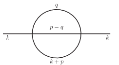
Figure 9: Third topology for two-loop self-energy

$$\Pi_{e}^{C}=\oint_{C}\frac{dp_{0}}{2\pi i}\oint_{C}\frac{dq_{0}}{2\pi i}\frac{f^{C}(p_{0},q_{0})}{(p_{0}^{2}-w^{2})[(p_{0}-q_{0})^{2}-z^{2}](q_{0}^{2}-y^{2})},$$ (60)

with the notation $w=|\vec{p}+\vec{k}|$, $y=|\vec{q}|$ and $z=|\vec{p}-\vec{q}|$.

Performing the integration in $p_{0}$, with the help of the residue theorem, we obtain

$$\Pi_{e}^{C} =-\oint_{C}\frac{dq_{0}}{2\pi i}\left\{\left[\frac{f^{C}(w,q_{0})}{2w[(w-q_{0})^{2}-z^{2}](q_{0}^{2}-y^{2})}\right.\right.$$

$$+\left.\left.\frac{f^{C}(q_{0}+z,q_{0})}{2z[(q_{0}+z)^{2}-w^{2}](q_{0}^{2}-y^{2})}\right]+[w,z\rightarrow-w,-z]\right\}.$$ (61)

Similarly, the integration in $q_{0}$ yields

$$\Pi_{e}^{C} =\left\{\left[\frac{f^{C}(w,y)}{4wy[(w-y)^{2}-z^{2}]}+\frac{f^{C}(y+z,y)}{4zy[(y+z)^{2}-w^{2}]}\right.\right.$$

$$+\left.(y\rightarrow-y)\right]+\left[\frac{f^{C}(w,w+z)}{4wz[(w+z)^{2}-y^{2}]}+(z\rightarrow-z)\right]$$

$$+\left.\left[\frac{f^{C}(w,w-z)}{4zw[(w-z)^{2}-y^{2}]}+(w\rightarrow-w)\right]\right\}$$

$$+\{w,z\rightarrow-w-z\}.$$ (62)

In the high-temperature limit we consider $w=x+\epsilon$, with $x=|\vec{p}|$, so that the dominant term is

$$\Pi_{e}^{C} \simeq\left\{\left[\frac{f^{C}(x,y)}{4xy[(x-y)^{2}-z^{2}]}+\frac{f^{C}(y+z,y)}{4zy[(y+z)^{2}-x^{2}]}\right.\right.$$

$$+\left.(y\rightarrow-y)\right]+\left[\frac{f^{C}(x,x+z)}{4xz[(x+z)^{2}-y^{2}]}+(z\rightarrow-z)\right]$$

$$+\left.\left[\frac{f^{C}(x,x-z)}{4zx[(x-z)^{2}-y^{2}]}+(x\rightarrow-x)\right]\right\}$$

$$+\{x,z\rightarrow-x-z\}$$

$$=\oint_{C}\frac{dp_{0}}{2\pi i}\oint_{C}\frac{dq_{0}}{2\pi i}\frac{f^{C}(p_{0},q_{0})}{(p_{0}^{2}-x^{2})[(p_{0}-q_{0})^{2}-z^{2}](q_{0}^{2}-y^{2})}$$

$$=\Pi_{0}^{C},$$ (63)

where we identify the zero-momentum limit of the amplitude

$$\Pi_{0}^{C} =\oint_{C}\frac{dp_{0}}{2\pi i}\oint_{C}\frac{dq_{0}}{2\pi i}\frac{f^{C}(p_{0},q_{0})}{(p_{0}^{2}-x^{2})[(p_{0}-q_{0})^{2}-z^{2}](q_{0}^{2}-y^{2})},$$ (64)

which establishes the SZM identity for this amplitude.

A.2 Fourth topology

Let us now consider the topology shown in Fig. 10 which, in the static limit, has the following form

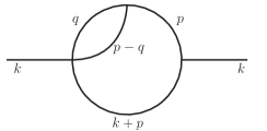
Figure 10: Fourth topology for two-loop self-energy

$$\Pi_{e}^{D}=\oint_{C}\frac{dp_{0}}{2\pi i}\oint_{C}\frac{dq_{0}}{2\pi i}\frac{f^{D}(p_{0},q_{0})}{(p_{0}^{2}-x^{2})(p_{0}^{2}-w^{2})[(p_{0}-q_{0})^{2}-z^{2}](q_{0}^{2}-y^{2})},$$ (65)

where we are using the notation $x=\left|\vec{p}\right|$, $y=\left|\vec{q}\right|$, $w=|\vec{p}+\vec{k}|$ and $z=\left|\vec{p}-\vec{q}\right|$.

As before, we employ the residue theorem to perform the integration in $p_{0}$ and in $q_{0}$, obtaining

$$\Pi_{e}^{D} =\left\{\left[\frac{f^{D}(x,y)}{4xy(x^{2}-w^{2})[(x-y)^{2}-z^{2}]}+\frac{f^{D}(w,y)}{4wy(w^{2}-x^{2})[(w-y)^{2}-w^{2}]}+\frac{f^{D}(y+z,y)}{4zy[(y+z)^{2}-x^{2}][(y+z)^{2}-w^{2}]}\right.\right.$$

$$+\left.(y\rightarrow-y)\right]+\left[\frac{f^{D}(x,x+z)}{4zx(x^{2}-w^{2})[(x+z)^{2}-y^{2}]}+\frac{f^{D}(w,w+z)}{4zw(w^{2}-x^{2})[(w+z)^{2}-y^{2}]}+(z\rightarrow-z)\right]$$

$$+\left[\frac{f^{D}(x,x-z)}{4xz(x^{2}-w^{2})[(x-z)^{2}-y^{2}]}+(x\rightarrow-x)\right]+\left.\left[\frac{f^{D}(w,w-z)}{4wz(w^{2}-x^{2})[(w-z)^{2}-y^{2}]}+(w\rightarrow-w)\right]\right\}$$

$$+\{(x,w,z)\rightarrow(-x,-w,-z)\}.$$ (66)

In the high-temperature limit, the relation in Eq. (4) yields

$$\Pi_{e}^{D} \simeq\left\{\left[\frac{1}{2x}\frac{\partial}{\partial x}\frac{f^{D}(x,y)}{4xy[(x-y)^{2}-z^{2}]}+\frac{f^{D}(y+z,y)}{4zy[(y+z)^{2}-x^{2}]^{2}}+(y\rightarrow-y)\right]+\left[\frac{1}{2x}\frac{\partial}{\partial x}\frac{f^{D}(x,x+z)}{4zx[(x+z)^{2}-y^{2}]}+(z\rightarrow-z)\right]\right.$$

$$+\left.\left[\frac{1}{2x}\frac{\partial}{\partial x}\frac{f^{D}(x,x-z)}{4xz[(x-z)^{2}-y^{2}]}+(x\rightarrow-x)\right]\right\}+\{(x,z)\rightarrow(-x,-z)\}.$$ (67)

On the other hand, the zero external four-momentum amplitude is

$$\Pi_{0}^{D}=\oint_{C}\frac{dp_{0}}{2\pi i}\oint_{C}\frac{dq_{0}}{2\pi i}\frac{f^{D}(p_{0},q_{0})}{(p_{0}^{2}-x^{2})^{2}[(p_{0}-q_{0})^{2}-z^{2}](q_{0}^{2}-y^{2})}.$$ (68)

Using the residue theorem, the integration in $p_{0}$ gives

$$\Pi_{0}^{D} =-\oint_{C}\frac{dq_{0}}{2\pi i}\left\{\left[\frac{f^{D}(q_{0}+z,q_{0})}{2z[(q_{0}+z)^{2}-x^{2}]^{2}(q_{0}^{2}-y^{2})}\right.\right.$$

$$+\left.\frac{1}{2x}\frac{\partial}{\partial x}\frac{f^{D}(x,q_{0})}{2x[(x-q_{0})^{2}-z^{2}](q_{0}^{2}-y^{2})}\right]$$

$$+\left.\left[(x,z)\rightarrow(-x,-z)\right]\right\}.$$ (69)

Similarly, the integration in $q_{0}$ produces

$$\Pi_{0}^{D} =\left\{\left[\frac{f^{D}(y+z,y)}{4zy[(y+z)^{2}-x^{2}]^{2}}\right.\right.$$

$$+\left.\frac{1}{2x}\frac{\partial}{\partial x}\frac{f^{D}(x,y)}{4xy[(x-y)^{2}-z^{2}]}+(y\rightarrow-y)\right]$$

$$+\left[\frac{1}{2x}\frac{\partial}{\partial x}\frac{f^{D}(x,x+z)}{4xz[(x+z)^{2}-y^{2}]}+(z\rightarrow-z)\right]$$

$$+\left.\left[\frac{1}{2x}\frac{\partial}{\partial x}\frac{f^{D}(x,x-z)}{4zx[(x-z)^{2}-y^{2}]}+(x\rightarrow-x)\right]\right\}$$

$$+\{(x,z)\rightarrow(-x,-z)\}.$$ (70)

Comparing the static limit [(67)] with the zero momentum limit [(70)] we can verify the SZM identity for the amplitude shown in Fig. 10.

A.3 Fifth topology

The fifth topology for the two-loop self-energy is shown in Fig. 11. In the static limit it reduces to

$$\Pi_{e}^{E}=\oint_{C}\frac{dp_{0}}{2\pi i}\oint_{C}\frac{dq_{0}}{2\pi i}\frac{f^{E}(p_{0},q_{0})}{(p_{0}^{2}-x^{2})^{2}(p_{0}^{2}-w^{2})(q_{0}^{2}-y^{2})},$$ (71)

with $x=\left|\vec{p}\right|$, $y=\left|\vec{q}\right|$ and $w=|\vec{p}+\vec{k}|$.

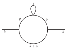
Figure 11: Fifth topology for two loops self energy.

Performing the integration in $p_{0}$ with the help of the residue theorem, we obtain

$$\Pi_{e}^{E} =-\oint_{C}\frac{dq_{0}}{2\pi i}\left\{\frac{f^{E}(w,q_{0})}{2w(w^{2}-x^{2})^{2}(q_{0}^{2}-y^{2})}\right.$$

$$+\left.(w\rightarrow-w)\right.$$

$$+\left.\frac{1}{2x}\frac{\partial}{\partial x}\frac{f^{E}(x,q_{0})}{2x(x^{2}-w^{2})(q_{0}^{2}-y^{2})}\right.$$

$$+\left.(x\rightarrow-x)\right\}.$$ (72)

In this amplitude the internal loops do not overlap, and therefore it is not necessary, for the present purpose, to perform the $q_{0}$ integration.

In the high-temperature limit we can use the approximation in Eq. (52) and the identity in Eq. (54) which lead to

$$\Pi_{e}^{E} \simeq-\oint_{C}\frac{dq_{0}}{2\pi i}\left\{\frac{3}{16x^{5}}\frac{f^{E}(x,q_{0})}{(q_{0}^{2}-y^{2})}\right.$$

$$-\left.\frac{3}{16x^{4}}\frac{\partial}{\partial x}\frac{f^{E}(x,q_{0})}{(q_{0}^{2}-y^{2})}+\frac{1}{16x^{3}}\frac{\partial^{2}}{\partial x^{2}}\frac{f^{E}(x,q_{0})}{(q_{0}^{2}-y^{2})}\right.$$

$$+\left.(x\rightarrow-x)\right\}.$$ (73)

When all the external four-momentum vanish, the amplitude reduces to

$$\Pi_{0}^{E}=\oint_{C}\frac{dp_{0}}{2\pi i}\oint_{C}\frac{dq_{0}}{2\pi i}\frac{f^{E}(p_{0},q_{0})}{(p_{0}^{2}-x^{2})^{3}(q_{0}^{2}-y^{2})}.$$ (74)

Using the residue theorem in order to perform the $p_{0}$ integration, we obtain

$$\Pi_{0}^{E} =-\oint_{C}\frac{dq_{0}}{2\pi i}\left[\frac{1}{2}\lim_{p_{0}=x}\frac{\partial^{2}}{\partial p_{0}^{2}}\frac{f^{E}(p_{0},q_{0})}{(p_{0}+x)^{3}(q_{0}^{2}-y^{2})}\right.$$

$$+\left.(x\rightarrow-x)\right].$$ (75)

Finally, computing the limit, we obtain

$$\Pi_{0}^{E} =-\oint_{C}\frac{dq_{0}}{2\pi i}\left\{\frac{3}{16x^{5}}\frac{f^{E}(x,q_{0})}{(q_{0}^{2}-y^{2})}-\frac{3}{16x^{4}}\frac{\partial}{\partial x}\frac{f^{E}(x,q_{0})}{(q_{0}^{2}-y^{2})}\right.$$

$$+\left.\frac{1}{16x^{3}}\frac{\partial^{2}}{\partial x^{2}}\frac{f^{E}(x,q_{0})}{(q_{0}^{2}-y^{2})}+(x\rightarrow-x)\right\}.$$ (76)

Therefore, the static result [(73)] together with the zero-momentum result [(76)] implies the SZM identity for the topology shown in Fig. 11.

References

- Braaten and Pisarski (1990a) E. Braaten and R. D. Pisarski, Nucl. Phys. B337, 569 (1990a); B339, 310 (1990b).
- Frenkel and Taylor (1990) J. Frenkel and J. C. Taylor, Nucl. Phys. B334, 199 (1990); B374, 156 (1992).
- Kapusta (1989) J. I. Kapusta, Finite Temperature Field Theory (Cambridge University Press, Cambridge, England, 1989).
- Bellac (1996) M. L. Bellac, Thermal Field Theory (Cambridge University Press, Cambridge, England, 1996).
- Brandt et al. (2009) F. T. Brandt, J. Frenkel, D. G. C. McKeon, and J. B. Siqueira, Phys. Rev. D 80, 025024 (2009).
- Brandt et al. (2006) F. T. Brandt, J. Frenkel, and C. Muramoto, Nucl. Phys. B754, 146 (2006).
- Brandt and Frenkel (1993) F. T. Brandt and J. Frenkel, Phys. Rev. D 47, 4688 (1993).
- Brandt et al. (1995) F. T. Brandt, J. Frenkel, and J. C. Taylor, Nucl. Phys. B437, 433 (1995).
- Brandt and Siqueira (2012) F. T. Brandt and J. B. Siqueira, Phys. Rev. D 85, 067701 (2012).
- Frenkel et al. (2009) J. Frenkel, S. H. Pereira, and N. Takahashi, Phys. Rev. D 79, 085001 (2009).
- (11) F. T. Brandt, J. Frenkel and J. C. Taylor, Nucl. Phys. B 814, 366 (2009).
- (12) E. Mottola and Z. Szep, Phys. Rev. D 81, 025014 (2010).