A Modified Histogram Method for Disordered Lattices

Abstract

A new method is developed to extend the histogram method [1, 2] to lattices with any type of disorder. The Monte Carlo single- and multiple-histogram methods were developed to get the most out of only a few simulations, but are restricted to simulations with identical lattice configurations. The method introduced here expands on the histogram method to allow data from various disordered lattice configurations to be optimally combined in a single weighted average result. This method is applied to a simple Ising-like model of the relaxor ferroelectric perovskite solid solution $BaTiO_{3}$ - $Bi(Zn_{1/2}Ti_{1/2})O_{3}$ (BT-BZT), in which disorder plays a pivotal role.

1 Introduction

Studying phase transitions using Monte Carlo simulations can be challenging. Various analysis methods have been developed, especially for simple systems such as the Ising[3, 4, 5] , Potts[6, 7, 8], and Heisenberg models[9, 10]. These methods can be expanded to more complex systems, but there are limitations. One thing that most Ising-like models have in common is a homogeneous lattice, where each cell has the same accessible magnetic states. A useful tool for analyzing Monte Carlo data for systems like this is the histogram method developed by Ferrenberg and Swendsen[1, 2]. The histogram method allows for only a few simulations to be performed, while maintaining a high level of accuracy in the calculations. As long as the necessary accessible states are sufficiently sampled, the accuracy of the calculations remains high. For a traditional Ising model, the histogram method uses a histogram that is populated from accessible energy and magnetization states to calculate the probability that the system will end up in a particular state. Several studies using the histogram methods[9, 11, 12, 10] have shown promise in improving the temperature resolution without increased computational time.

A modified histogram method is introduced to analyze phase transitions of an Ising-like model in which the system is disordered and contains cells with different accessible states. One drawback of the histogram method is that it is constrained to combining data from simulations of homogeneous lattices of the same size. The new method allows simulations of differing lattice size to be combined in a similar fashion, as well as allowing for the combination of inhomogeneous disordered lattices.

The modified method is tested on a system—a solid solution relaxor ferroelectric—containing cells with electric dipoles, instead of the traditional magnetic dipoles. Therefore, the measurables of the system are energy and polarization, $E$ and $\vec{p}$. The method applies for computation of any thermal average of a function of $E$ and $\vec{p}$ can be calculated. See Section 7 for more details on the solid solution used as a test case. In this context, the histograms will be populated with energies and polarizations, instead of the usual energies and magnetizations.

2 Single Histogram Method

A conventional Monte Carlo simulation involves generating a set of $N$ samples that represent the canonical ensemble at a temperature $T$. From this set of samples, the mean value of any function of the energy and polarization may be found using the equation

$$\langle f(E,\vec{p})\rangle=\frac{1}{N}\sum_{i=1}^{N}f(E_{i},\vec{p}_{i})\;,$$ (1)

where the subscript $i$ is the index of a particular data sample, and $N$ is the total number of samples. Unfortunately, this method only gives results at the temperature used to create the sampled data. Thus, a computationally expensive Monte Carlo simulation must be run for each temperature of interest. Using the single histogram method, the data from a simulation at one temperature may be used to predict properties at other similar temperatures[1].

The histogram method was created to extract as much information as possible from a Monte Carlo simulation, while minimizing the computational effort. This technique relies on the fact that if the probability of finding the system in each microstate at a given temperature is precisely known, then in principle the probability of finding the system in any of those microstates at any other temperature can be predicted. In practice, these probabilities can only be approximated, and calculated temperatures must be relatively close to simulated temperatures in order to achieve statistically significant results.

The histogram method begins with constructing a histogram of microstates $H(E,\vec{p})$, from a Monte Carlo simulation at a single temperature. For the simple Ising model, this histogram has a natural resolution in terms of both energy and magnetization, with the resolution determined by the change in each of these quantities due to a single cell flip. In this paper, consideration is given to disorder in the number of polarization states available in each cell, complicating the choice of bin size. These bin size effects are discussed in more detail in Section 4. The summations below are summations over the energy and polarization bins of the histogram.

The single histogram method is used to calculate the probability of finding the system in a particular microstate at a similar desired temperature $T$, different from the temperature $T_{0}$ at which the simulation was performed. The probability is given by

$$P_{\beta}(E,\vec{p})=\frac{1}{Z_{\beta}}H(E,\vec{p})\exp(-(\beta-\beta_{0})(E-\vec{p}\cdot\vec{E}))\;,$$ (2)

where $\beta_{0}=1/(k_{B}T_{0})$, $\beta=1/(k_{B}T)$, $\vec{E}$ is the external applied electric field, and $Z_{\beta}$ is a the partition function given by

$$Z_{\beta}=\sum_{E,\,\vec{p}}H(E,\vec{p})\exp(-(\beta-\beta_{0})(E-\vec{p}\cdot\vec{E}))\;.$$ (3)

The mean value of any quantity at the desired temperature is then found using,

$$\langle f(E,\vec{p})\rangle_{\beta}=\sum_{E,\,\vec{p}}f(E,\vec{p})P_{\beta}(E,\vec{p})\;.$$ (4)

This technique is accurate if the desired temperature $T$ is near the simulation temperature $T_{0}$, but becomes increasingly imprecise as the temperature $T$ deviates from $T_{0}$, and the population $P_{\beta}(E,\vec{p})$ becomes increasingly different from $H(E,\vec{p})$. Details of this uncertainty are discussed in Section 6.

3 Multiple Histogram Method

When computing the value of a property over a large range of temperatures, the single histogram method becomes sub-optimal. Each calculation uses data from only a single simulation temperature histogram. When examining a temperature precisely between two simulation temperatures, it would be ideal to use data from both of those simulations. The multiple-histogram method addresses this issue, and allows for the use of all the Monte Carlo simulation data for each computed data point. Similar uncertainties are achieved with similar computational effort by either simulating many temperatures with fewer iterations at each temperature, or by running simulations at fewer temperatures with more iterations in each simulations. Thus the multiple-histogram method serves as an optimal interpolation scheme for examining intermediate temperatures. This allows for more precise results, and leads to greatly reduced computation time.

The multiple histogram method as proposed by Ferrenberg and Swendsen [2], uses the following equation for the probability function at temperature $T$:

$$\tilde{P}_{\beta}(E,\vec{p})=\frac{\sum_{n=1}^{N}H_{n}(E,\vec{p})g_{n}^{-1}\exp\left(-\beta E\right)}{\sum_{m=1}^{N}n_{m}g_{m}^{-1}\exp\left(-\beta_{m}E-f_{m}\right)}\;,$$ (5)

where $\beta_{m}=1/k_{B}T_{m}$, $N$ is the number of simulations, $H_{m}(E,\vec{p})$ is the histogram of the $m^{th}$ simulation, $n_{m}$ is the total number of samples included in the $m^{th}$ histogram, $g_{m}=1+2\tau_{m}$ with $\tau_{m}$ being the correlation time, and $f_{m}$ is an estimate of the dimensionless free energy of the $m^{th}$ simulation, discussed below. The correlation time serves as a weighting factor to account for the differing correlation times of the samples for different simulations, which affects the number of statistically distinct configurations present. The free energies serve as a correction factor due to combining data from multiple temperatures, and are calculated self consistently using

$$\exp\left(f_{m}\right)=\tilde{P}_{\beta_{m}}(E,\vec{p})\;.$$ (6)

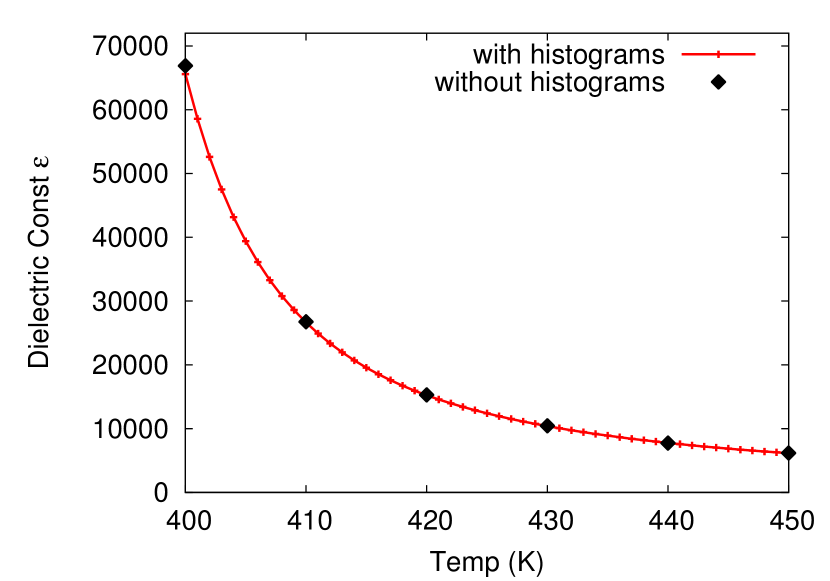
(a) Dielectric constant with and without multiple-histogram method

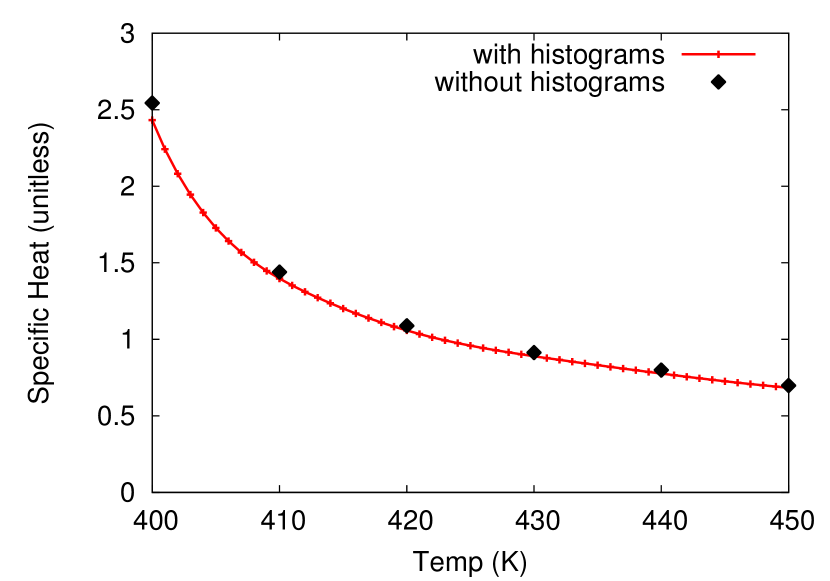
(b) Specific heat with and without multiple-histogram method

Figure 1: [Color online] Dielectric constant and Specific Heat of a homogeneous $16\times 16\times 16$ lattice using raw data and the multiple histogram method. The simulations used for the non-histogram method are also the inputs in the multiple histogram method. The multiple histogram method is sampled every 1K, while the input simulations were performed every 10K.

Note that Equation 5 does not give the actual probability, but a probability distribution function that is unnormalized. To normalize the distribution function and obtain an actual probability, it is just a matter of dividing by another partition function:

$$P_{\beta}(E,\vec{p})=\frac{\tilde{P}_{\beta}(E,\vec{p})}{\sum_{E,\vec{p}}\tilde{P}_{\beta}(E,\vec{p})}\;.$$ (7)

Once the probabilities are determined, the mean value of a quantity is once again calculated using Equation 4. To illustrate the interpolation benefits of the multiple-histogram method, Figure 1 compares the dielectric constant and specific heat of a $16\times 16\times 16$ homogeneous lattice for simulations at every 10 Kelvin and the multiple-histogram method using the data from the same input simulations. The specific heat and electric susceptibility are essentially the variance of the energy and polarization respectively:

$$c=\frac{\beta^{2}}{N}\left(\langle E^{2}\rangle-\langle E\rangle^{2}\right)\;,$$ (8)

where $N$ is the number of cells in the lattice, and

$$\chi=\beta\left(\langle P^{2}\rangle-\langle P\rangle^{2}\right)\;.$$ (9)

Note that $\chi$ is a tensor value, and only a single independent direction may be calculated at once. The dielectric constant may also be calculated using

$$\epsilon=1+4\pi\chi\;.$$ (10)

4 Histogram Bin Size

The bin size that determines the allowable microstates for energy and polarization is not as easily defined for inhomogeneous lattices as it is for the simple Ising model. For the inhomogeneous model, instead of calculating every possible microstate of energy and polarization, a standard bin size is used because different lattice configurations may have different sets of available energy and polarization microstates. This also allows for data from multiple simulations to be combined in a straight-forward manner. The bin size used here is determined by calculating the energy and polarization differences for a single flip of the cells with the smallest polarization. The histogram is then filled with the simulation data according to the smallest bin sizes.

Larger bin sizes are less computationally expensive than small bins, since the mean value of any function of $E$ and $\vec{p}$ is a sum over the available microstates. More bins means more microstates, and more microstates amount to more computational time. However, there is a limit to the maximum size a bin may be before the technique loses accuracy. The smallest bin size that should be used is that which corresponds to the difference in energy or polarization due to flipping a single cell from one state to another. The dielectric constant is the variance of the polarization, and thus depends only on the bin size of the polarizations. Similarly, the specific heat only depends on the bin size of the energy. A simple test for the application used here reveals that the maximum accurate bin size for both energy and polarization occurs at about four times the minimum bin size.

5 Combining Histograms of Different Configurations

The multiple-histogram method addresses the possibility of combining together simulations at several temperatures in order to reduce the statistical errors associated with the number of iterations simulated. When studying a disordered material such as a solid solution, there is another sort of statistical error, which arises from the lattice size. This could be addressed by simulating a very large lattice, but the statistical error only drops as the square root of the size of the lattice. If the lattice size of a completed simulation is determined to be too small, it is discouraging to start again with a larger lattice, losing the computational effort on the original lattice. The new approach discussed here combines simulations from distinct lattices that differ in disorder as well as lattice size, so as to provide improved statistical averaging over all disordered configurations. While the conventional multiple-histogram method combines simulations at different temperatures, the new modified histogram method combines simulations in different lattice configurations and temperatures, to provide better statistical averaging of disordered materials.

Consider the case of two systems with the same lattice size that represent the same system, with different disordered lattice configurations. The two systems may be combined into one large system with twice the volume and number of cells of each original system. To get accurate results for this larger system, the probabilities are calculated for the new larger system and are used to obtain the averaged values from Equation 4. Instead of running the full Monte Carlo simulation of the larger cell, the probability of finding each microstate of the large cell is approximated using the probability distributions of the smaller subsystems.

In general, the probability of finding multiple configurations each with a particular energy is the product of the individual probabilities

$$P_{tot}(E_{1},E_{2},\cdots,E_{n})=P_{1}(E_{1})P_{2}(E_{2})\cdots P_{N}(E_{n})\;,$$ (11)

where $P_{i}(E_{j_{i}})$ is the probability of finding system $i$ with energy $E_{i}$, under the assumption that the systems may be considered non-interacting and statistically independent. For brevity, the discussion here is only focused on the energy of the system, but the method is trivially extended to include polarization or magnetization.

To describe a system that combines multiple systems together into a larger volume, the resulting probability must be a function of the total energy, rather than the energy of each subsystem as in Equation 11. This is accomplished by integrating over all energy microstates with an appropriate delta function constraining the total energy

$$P_{tot}(E_{tot}) =\int dE_{1}\int dE_{2}\cdots\int dE_{n}P_{1}(E_{j_{1}})P_{2}(E_{j_{2}})\cdots P_{N}(E_{j_{n}})\delta(E-(E_{1}+E_{2}+\cdots+E_{n}))\;.$$ (12)

Considering only discrete states and including the polarization dimension as well, the combined probability becomes

$$\begin{split}P_{\beta,tot}\left(E,\vec{p}\right)=\sum_{E_{1},\vec{p}_{1}}\sum_{E_{2},\vec{p}_{2}}\cdots\sum_{E_{n},\vec{p}_{n}}P_{\beta,1}\left(E_{1},\vec{p}_{1}\right)P_{\beta,2}\left(E_{2},\vec{p}_{2}\right)\cdots P_{\beta,N}\left(E_{N},\vec{p}_{N}\right)\\ \delta_{E,(E_{1}+E_{2}+\cdots+E_{N})}\delta_{\vec{p},(\vec{p}_{1}+\vec{p}_{2}+\cdots+\vec{p}_{N})}\;,\end{split}$$ (13)

where the subscript $\beta$ indicates the dependence of probability on temperature.

One challenge that arises when calculating the total probability this way is that it is computationally expensive. If each sum is order $\mathcal{O}(M)$, where $M$ is the number of energy and polarization microstates for an individual lattice configuration, and the total probability is a combination of $N$ lattice configurations, the resulting probability calculation is order $\mathcal{O}(M^{N})$. This can be a serious performance issue when combining more than just a few lattice configurations. Convolutions are used to speed up the computational process.

A convolution of two functions $f(t)$ and $g(t)$ is defined as

$$(f\circ g)(t)\equiv\int_{-\infty}^{\infty}f(\tau)g(t-\tau)d\tau\;.$$ (14)

To quickly calculate convolutions, the convolution theorem is utilized:

$$\mathcal{F}[f\circ g]=\mathcal{F}[f]\cdot\mathcal{F}[g]\;,$$ (15)

where $\mathcal{F}$ represents a Fourier transform. Recognizing the similarity between the new total probability, given in Equation 13, and a series of convolutions allows for the use of the advantageous discrete Fourier transforms to calculate the final unnormalized probability:

$$\begin{split}\tilde{P}_{\beta,tot}\left(E,\vec{p}\right)&=\mathcal{F}^{\;-1}\Big{[}\mathcal{F}[P_{\beta,1}\left(E_{1},\vec{p}_{1}\right)]\times\\ &\mathcal{F}[P_{\beta,2}\left(E_{2},\vec{p}_{2}\right)]\times\cdots\times\mathcal{F}[P_{\beta,N}\left(E_{N},\vec{p}_{N}\right)]\Big{]}\;.\end{split}$$ (16)

The final normalized probability is found using Equation 7.

In order to use the Fourier transform technique, each individual probability must have the same number of microstates as the total probability. As was previously stated, the number of microstates of the final probability is of order $\mathcal{O}(M^{N})$. This number can be dramatically reduced by making the bins of each individual histogram, and subsequently each polarization, conform to the same microstate grid. If each histogram has the same bin size and is centered on the same values, the number of microstates of the final polarization can be reduced to

$$M_{E_{total}} =\Big{[}M_{E_{1}}+M_{E_{2}}+\cdots+M_{E_{N}}-(N-1)\Big{]}\;,$$ (17)

$$M_{\vec{p}_{total}} =\Big{[}M_{\vec{p}_{1}}+M_{\vec{p}_{2}}+\cdots+M_{\vec{p}_{N}}-(N-1)\Big{]}\;,$$ (18)

$$M =M_{E_{total}}\times M_{\vec{p}_{total}}\;,$$ (19)

where $M_{E_{i}}$, $M_{\vec{p}_{i}}$ are the number of energy and polarization microstates of the $i^{th}$ lattice configuration respectively, and $N$ is the number of lattice configurations being combined. To calculate the total probability of Equation 13, there are $N$ convolutions required and $3N$ FFTs per convolution. Each FFT is of order $\mathcal{O}(M\log M)$, so the total probability calculation is of order $\mathcal{O}(N\times M\log M)$. When combining many simulations, or even a few simulations with many bins, this can be computationally intensive.

6 Uncertainties

The level of accuracy in any computed quantity is always of great importance, and the multiple histogram method is no exception. In general, Monte Carlo methods have the advantage of begin able to produce rigorous statistical error bars. The statistical uncertainty of the multiple histogram probability is given by

$$\delta P_{\beta}\left(E,\vec{p}\right)=\left(\sum_{n=1}^{N}\frac{H_{n}\left(E,\vec{p}\right)}{g_{n}}\right)^{-1/2}P_{\beta}\left(E,\vec{p}\right)\;,$$ (20)

where the sum is over all $N$ simulations, $H_{n}(E,\vec{p})$ is the histogram of a single simulation, and $g_{n}=1+2\tau_{n}$ is the correlation time factor [2].

The form of Equation 20 is similar to that of any counting experiment, with a relative uncertainty $(\delta P/P)$ proportional to $1/\sqrt{N}$. Just as more counts reduce the uncertainty in any normal counting experiment, more counts per bin of each histogram reduce the statistical error in the probabilities. If the relative uncertainty is high, more Monte Carlo data must be obtained to fill in the gaps for those microstates. The relative uncertainty should be low for the entire range of occupied microstates in order to produce reliable results at a given temperature. Figure 2 shows the relative uncertainty of Equation 20 using both two and three simulation temperatures. The relative uncertainty with only two simulations has a region of high uncertainty, while adding a third simulation reduces the uncertainty for a larger temperature range. The uncertainty at the end points diverges as there are no occupied microstates far from the simulated temperatures.

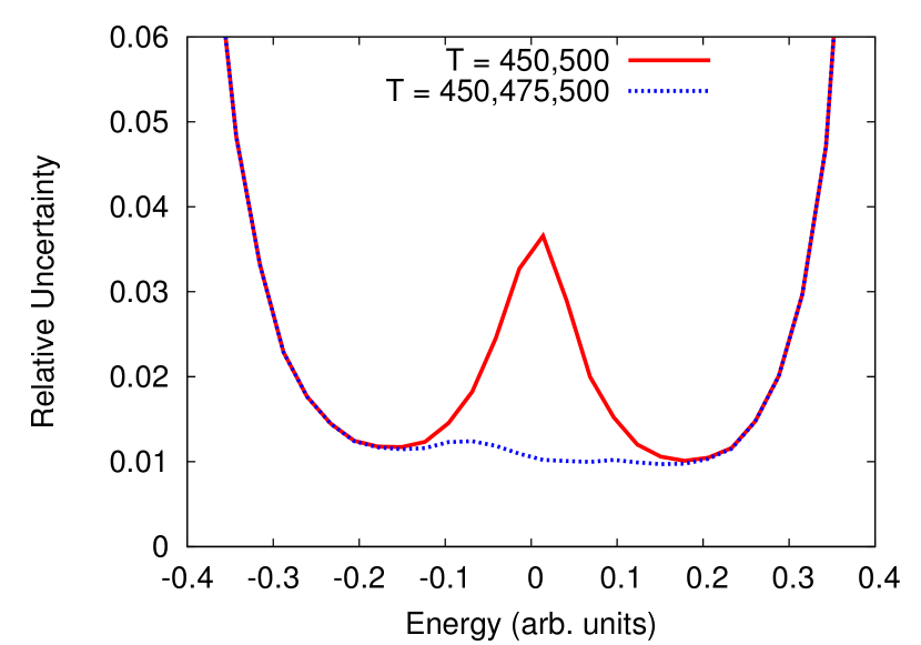
Figure 2: [Color online] The relative uncertainty for two different multiple histograms. One with simulations at T=450,500K, and the other with simulations at T=450,475,500K. The relative uncertainty with only two simulations has a region of higher uncertainty. Adding a third simulation to the histogram data lowers the uncertainty in the center region so the relative uncertainty of the probability for the entire valid region is less than 2%.

Another source of error in histogram re-weighting is due to using a finite number of samples in the histogram. For an excellent discussion of errors associated with the histogram method, see Newman and Palmer[13], who discuss this error in detail. As long as the histograms of every simulation temperature have sufficient overlap, the finite sample error will be small for the entire temperature range. Figure 3 shows the overlap of three histograms at different simulation temperatures. If the amount of overlap is sufficient, the finite sample error will be small because the number of counts in each bin of the histogram is large. At the end points of the histogram the finite sample error becomes large because the histogram is not filled in that region. This becomes extremely important if the histogram contains empty bins. According to Equation 20, the relative statistical uncertainty is infinite for microstates with empty bins. To avoid this problem, only data that has a reasonably high number of samples is used. Thus, the statistical error will dominate over finite sampling errors and remain finite. This may require more simulations or longer runs.

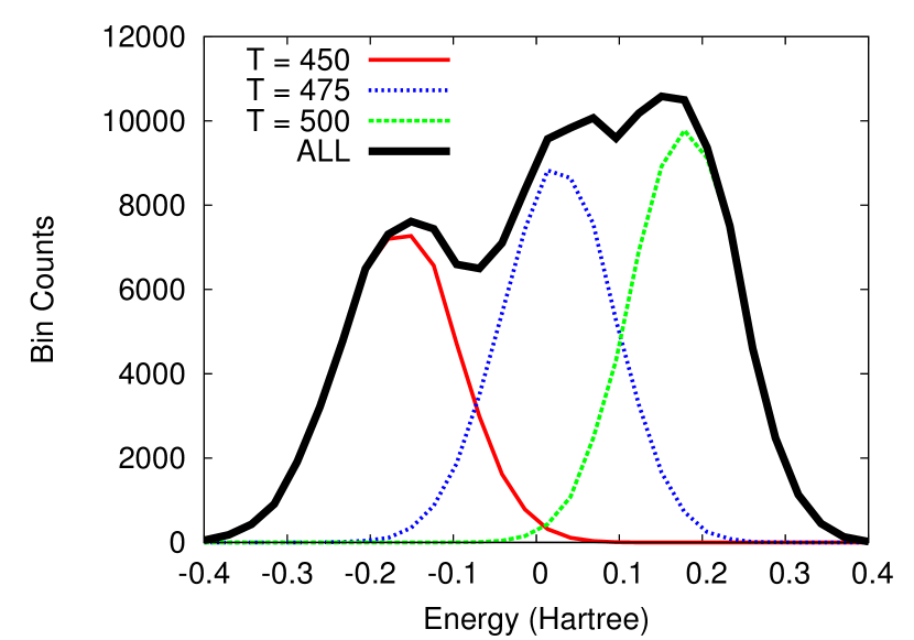
Figure 3: [Color online] Single and multiple energy histograms. Each of the three histograms have considerable overlap and combine to form one continuous multiple histogram. Sufficient overlap of histograms reduces the finite sample error.

Equation 20 gives the statistical error for the usual multiple-histogram method of Ferrenberg and Swendsen[2]. When combining multiple lattice configurations, the uncertainty equation must be modified in a way that is consistent with the combined probability of Equation 13. To make this clear, a shorthand for the probability in Equation 13 is introduced as

$$P_{tot}=\sum_{1}\sum_{2}\cdots\sum_{N}P_{1}P_{2}\cdots P_{N}\;,$$ (21)

where each summation is over the microstates of the probabilities of the same subscript, and the delta functions are simply implied. The uncertainty in the total probability is then given by

$$\begin{split}\delta P_{tot}^{2}=\sum_{1}\left(\frac{\partial P}{\partial P_{1}}\delta P_{1}\right)^{2}&+\sum_{2}\left(\frac{\partial P}{\partial P_{2}}\delta P_{2}\right)^{2}+\cdots\\ &+\sum_{N}\left(\frac{\partial P}{\partial P_{N}}\delta P_{N}\right)^{2}\;,\end{split}$$ (22)

where the uncertainty for each lattice configuration $\delta P_{i}$ is calculated using Equation 20. This method is valid if each probability is independent, that is, the errors in probabilities are uncorrelated.

The derivative of Equation 21 with respect to a single lattice configuration probability is

$$\frac{\partial P}{\partial P_{i}}=\sum_{1}\cdots\sum_{i-1}\sum_{i+1}\cdots\sum_{N}P_{1}\cdots P_{i-1}P_{i+1}\cdots P_{N}\;.$$ (23)

The error in the total probability is then given by

$$\begin{split}\delta P_{tot}^{2}=\sum_{1}\Bigg{[}\left(\delta P_{1}\right)^{2}\left(\sum_{2}\sum_{3}\cdots\sum_{N}P_{2}P_{3}\cdots P_{N}\right)^{2}\Bigg{]}+\\ \sum_{2}\Bigg{[}\left(\delta P_{2}\right)^{2}\left(\sum_{1}\sum_{3}\cdots\sum_{N}P_{1}P_{3}\cdots P_{N}\right)^{2}\Bigg{]}+\cdots\\ +\sum_{N}\Bigg{[}\left(\delta P_{N}\right)^{2}\left(\sum_{1}\sum_{2}\cdots\sum_{N-1}P_{1}P_{2}\cdots P_{N-1}\right)^{2}\Bigg{]}\;.\end{split}$$ (24)

While this method is accurate considering the assumption that each probability is independent, it is computationally challenging, even when FFTs are used to do the convolutions. Since convolutions are essentially three discrete Fourier transforms, each convolution scales as that of an FFT, which is of order $\mathcal{O}{(M\log M)}$, with $M$ being the number of microstates and histogram bins. The uncertainty of the combined probability requires $N^{2}$ convolutions, thus the computational time is order $\mathcal{O}{(N^{2}\times M\log M)}$.

Once the total uncertainty $\delta P$ is found, the uncertainties in the polarization magnitude, specific heat, and dielectric constant may be determined. Here, the results are summarized for the uncertainty of each of the thermodynamic averages that are computed. First, consider the polarization magnitude. The uncertainty in the mean magnitude of polarization is given by

$$\delta\langle\,|\,\vec{p}\,|\,\rangle^{2}=\sum_{E,\vec{p}}\left(\frac{\partial\langle\,|\,\vec{p}\,|\,\rangle}{\partial P_{\beta}(E,\vec{p})}\delta P_{\beta}(E,\vec{p})\right)^{2}\;.$$ (25)

Taking the derivative of Equation 4 results in

$$\delta\langle\,|\,\vec{p}\,|\,\rangle^{2}=\sum_{E,\vec{p}}\left(\,|\,\vec{p}\,|\,-\langle\,|\,\vec{p}\,|\,\rangle\right)^{2}\left(\frac{\delta P}{Z}\right)^{2}\;.$$ (26)

The uncertainties of the susceptibility can be determined in the same manner as Equation 25,

$$\delta\chi^{2}=\sum_{E,\vec{p}}\left(\frac{\partial\chi\left(\vec{p}\right)}{\partial P_{\beta}\left(E,\vec{p}\right)}\delta P_{\beta}\left(E,\vec{p}\right)\right)^{2}.$$ (27)

By carrying out the derivative of Equation 9, and using the average values in the form of Equation 4, the resulting uncertainty in the susceptibility is given by

$$\begin{split}\delta\chi^{2}=\frac{\beta\,^{2}}{Z_{\beta}^{2}}\sum_{E,\vec{p}}\Big{[}\big{[}\vec{p}\;^{2}-\langle\vec{p}\;^{2}\rangle+2\langle\vec{p}\rangle\,^{2}-2\langle\vec{p}\rangle\,\vec{p}\big{]}^{2}\times\\ \left(\delta P_{\beta}\left(E,\vec{p}\right)\right)^{2}\Big{]}\;,\end{split}$$ (28)

and similarly for the specific heat,

$$\begin{split}\delta c^{2}=\frac{\beta\,^{4}}{M^{2}Z_{\beta}^{2}}\sum_{E,\vec{p}}\Big{[}\big{[}E\,^{2}-\langle E\,^{2}\rangle+2\langle E\rangle\,^{2}-2\langle E\rangle E\big{]}\,^{2}\times\\ \left(\delta P_{\beta}\left(E,\vec{p}\right)\right)^{2}\Big{]}\;,\end{split}$$ (29)

where $M$ is the number of cells on the lattice.

7 Application

The material that inspired this method is the solid solution $x\text{BaTiO}_{3}+(1-x)\text{Bi}(\text{Zn}_{1/2}\text{Ti}_{1/2})\text{O}_{3}$ (BT-BZT). For certain compositions, BT-BZT is a relaxor ferroelectric perovskite, which exhibits both long- and short-range disorder. At these compositions, BT-BZT features the so-called diffuse phase transition. For other compositions of BT-BZT behaves as a ferroelectric such as pure $BaTiO_{3}$, which maintains an ordinary ferroelectric phase transition.

The relaxor behavior is modeled using a combination of techniques including ab initio methods and an Ising-like model. The ab initio calculations are accurate at small length scales, but lack the ability to describe the necessary long-range interactions. The Ising-like model is able describe long-range effects, but cannot predict short-range interactions. By combining these methods into a single model, insight is gained about the larger picture by including both long- and short-range effects.

The ab initio calculations are restricted to $2\times 2\times 2$ supercells of BT-BZT for symmetry reasons. This allows for compositions of $x=0,0.25,0.5,0.75,1$, in the 40 atom supercell. Calculations are performed to determine the energies and polarizations of each unique configuration using the Quantum Espresso [14] package, Density Functional Theory (DFT) and the Modern Theory of Polarization (MTP) [15, 16, 17]. The DFT calculations were run using a PBE-GGA exchange-correlation functional, ultrasoft pseudopotentials, a cutoff energy of 80 Rydberg, and a $2\times 2\times 2$ Monkhorst-Pack $k$-point grid within the supercell. For all but $x=1$ there are multiple supercell configurations, each with multiple discrete polarization states. This disorder prompted the development of the new modified histogram method. For supercells with several polarization, each such state is treated within the Monte Carlo simulations.

After the energies and all polarization states of each $2\times 2\times 2$ configuration are determined for all compositions, this information is used to construct an Ising-like model. The classic Ising model for ferromagnetic systems has two states per lattice position: spin up and spin down[3, 4, 5]. The Heisenberg model improves this model by introducing a continuum of states, with the spin pointing in any direction. In this model, a lattice of $2\times 2\times 2$ supercells is used, which is populated with the atomic configurations discussed above. Each state has a set of possible polarizations determined by the ab initio calculations. The number of each type of $2\times 2\times 2$ supercells are determined using Boltzmann statistics at a formation temperature, and are distributed on the lattice stochastically. This differs from both Ising and Heisenberg models in that the polarizations are not simply up and down, but neither are they allowed to point in any direction. This adaptation is more closely related to the Potts model [6, 7, 8] in that there are several discrete directions of the polarizations, but unlike the Potts model the polarizations of the disordered lattice are not uniform in nature and each cell on the lattice may have different accessible polarization states.

The interaction Hamiltonian of the Heisenberg model used here is given by

$$H=-\frac{J}{2}\sum_{i}^{cells}\sum_{j}^{NN}\vec{p}_{i}\cdot\vec{p}_{j}-\sum_{i}^{cells}\vec{p}_{i}\cdot\vec{E}\;,$$ (30)

where $\vec{p}_{i}$ is the polarization of a single cell, $\vec{E}$ is the external electric field and $J$ is a coupling constant. The coupling constant is tuned to match the experimental Curie temperature of pure barium titanate using the fourth order Binder cumulant method [18]. This Hamiltonian does not take into account all of the long-range forces, but it is a good first approximation.

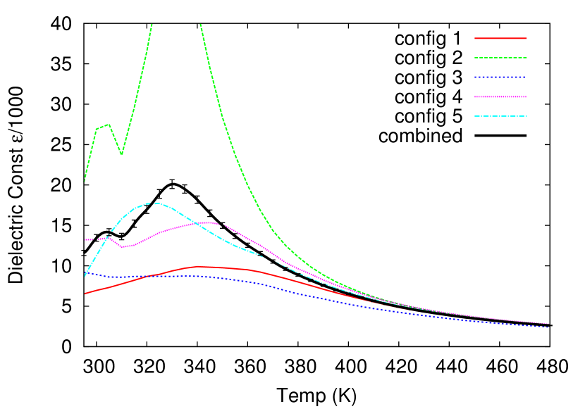
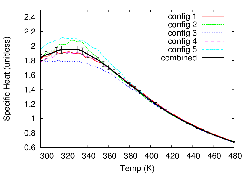
Figure 4: [Color online] The (a) dielectric constant and (b) specific heat for five different lattice configurations and the combined result with error bars for a composition of $x=0.95$.

Figure 4 shows the dielectric constant and specific heat for five different lattice configurations of BT-BZT, each with a composition of $x=0.95$, as well as the convolved combination of each configuration. Pure BTO ($x=1$) has a distinct phase transition near 380 K. As expected for a relaxor, the data in Figure 4 correctly shows that a sharp phase transition does not occur, and the material exhibits a diffuse phase transition. There is a large variation between individual configurations because the accessible energy and polarization microstates are different for each lattice configuration.

The combined result behaves very much like a weighted average of each individual result for both the specific heat and the dielectric constant. This is unsurprising, given that it corresponds to system composed of precisely these configurations. At high temperatures, where the results from each lattice configuration are very similar, the convolved results are quite smooth. At lower temperatures, there is quite a difference in the results for each lattice configuration, as the system freezes into different states according to the precise disordered state. The convolved results begin to smooth out compared to the results for an individual simulation, but there is a higher degree of uncertainty, and adding additional lattice configurations would reduce the uncertainty.

8 Conclusion and Summary

A modification of the multiple-histogram method for analysis of Monte Carlo data has been introduced. This new modification allows for easier and more efficient study of systems with a disordered lattice. The method was applied to a model of the relaxor ferroelectric perovskite solid solution $BaTiO_{3}$ - $Bi(Zn_{1/2}Ti_{1/2})O_{3}$ (BT-BZT). A total of 255 simulations were combined using the new modified histogram method to compute the specific heat and dielectric constant of this disordered material with improved accuracy and precision.

References

- [1] A. Ferrenberg, R. Swendsen, New Monte Carlo technique for studying phase transitions, Physical review letters 61 (23) (1988) 2635.
- [2] A. Ferrenberg, R. Swendsen, Optimized monte carlo data analysis, Physical Review Letters 63 (12) (1989) 1195–1198.
- [3] E. Ising, Beitrag zur theorie des ferromagnetismus, Zeitschrift für Physik A Hadrons and Nuclei 31 (1) (1925) 253–258.
- [4] L. Onsager, Crystal statistics. I. A two-dimensional model with an order-disorder transition, Physical Review 65 (3-4) (1944) 117.
- [5] M. Jensen, P. Bak, Mean-field theory of the three-dimensional anisotropic Ising model as a four-dimensional mapping, Physical Review B 27 (11) (1983) 6853.
- [6] R. Potts, Some generalized order-disorder transformations, in: Mathematical Proceedings of the Cambridge Philosophical Society, Vol. 48, Cambridge Univ Press, 1952, pp. 106–109.
- [7] B. Berg, H. Meyer-Ortmanns, A. Velytsky, Dynamics of phase transitions: The 3D 3-state Potts model, Physical Review D 70 (5) (2004) 054505.
- [8] A. Bazavov, B. Berg, S. Dubey, Phase transition properties of 3D Potts models, Nuclear Physics B 802 (3) (2008) 421–434.
- [9] P. Peczak, A. M. Ferrenberg, D. Landau, High-accuracy monte carlo study of the three-dimensional classical heisenberg ferromagnet, Physical Review B 43 (7) (1991) 6087.
- [10] K. Chen, A. Ferrenberg, D. Landau, Static critical behavior of three-dimensional classical Heisenberg models: A high-resolution Monte Carlo study, Physical Review B 48 (5) (1993) 3249.
- [11] A. Ferrenberg, D. Landau, R. Swendsen, Statistical errors in histogram reweighting, Physical Review E 51 (5) (1995) 5092.
- [12] A. Ferrenberg, D. Landau, Critical behavior of the three-dimensional Ising model: A high-resolution Monte Carlo study, Physical Review B 44 (10) (1991) 5081.
- [13] M. Newman, R. Palmer, Error estimation in the histogram Monte Carlo method, Journal of Statistical Physics 97 (5) (1999) 1011–1026.
-
[14]
P. G. et. al., QUANTUM ESPRESSO: a
modular and open-source software project for quantum simulations of
materials, Journal of Physics: Condensed Matter 21 (39) (2009) 395502
(19pp).
URL http://www.quantum-espresso.org - [15] R. King-Smith, D. Vanderbilt, Theory of polarization of crystalline solids, Physical Review B 47 (3) (1993) 1651.
- [16] D. Vanderbilt, R. King-Smith, Electric polarization as a bulk quantity and its relation to surface charge, Physical Review B 48 (7) (1993) 4442.
- [17] R. Resta, D. Vanderbilt, Theory of polarization: a modern approach, Physics of Ferroelectrics (2007) 31–68.
- [18] K. Binder, Critical properties from Monte Carlo coarse graining and renormalization, Physical Review Letters 47 (9) (1981) 693–696.