A Classical Density-Functional Theory for Describing Water Interfaces

Abstract

We develop a classical density functional for water which combines the White Bear fundamental-measure theory (FMT) functional for the hard sphere fluid with attractive interactions based on the Statistical Associating Fluid Theory (SAFT-VR). This functional reproduces the properties of water at both long and short length scales over a wide range of temperatures, and is computationally efficient, comparable to the cost of FMT itself. We demonstrate our functional by applying it to systems composed of two hard rods, four hard rods arranged in a square and hard spheres in water.

I Introduction

A large fraction of interesting chemistry—including all of molecular biology—takes place in aqueous solution. However, while quantum chemistry enables us to calculate the ground state energies of large molecules in vacuum, prediction of the free energy of even the smallest molecules in the presence of a solvent poses a continuing challenge due to the complex structure of a liquid and the computational cost of ab initio molecular dynamics car1985 ; grossman2004 . The current state-of-the art in ab initio molecular dynamics is limited to a few hundred water molecules per unit cell lewis2011doesnitric . On top of this, standard ab initio methods using classical molecular dynamics without van der Waals corrections strongly over-structure water, to the point that ice melts at over 400Kyoo2009phase ! There has been a flurry of recent publications implicating van der Waals effects as significant in reducing this over-structuringlin2009importance ; wang2011density ; mogelhoj2011ab ; jonchiere2011van . It has also been found that the inclusion of nuclear quantum effects can provide similar improvements morrone2008nuclear . Each of these corrections imposes an additional computational burden on an approach that is already feasible for only a very small number of water molecules. A more efficient approach is needed in order to study nanoscale and larger solutes.

I.1 Classical density-functional theory

Numerous approaches have been developed to approximate the effect of water as a solvent in atomistic calculations. Each of these approaches gives an adequate description of some aspect of interactions with water, but none of them is adequate for describing all these interactions with an accuracy close to that attained by ab initio calculations. The theory of Lum, Chandler and Weeks (LCW) lum1999hydrophobicity , for instance, can accurately describe the free energy cost of creating a cavity by placing a solute in water, but does not lend itself to extensions treating the strong interaction of water with hydrophilic solutes. Treatment of water as a continuum dielectric with a cavity surrounding each solute can give accurate predictions for the energy of solvation of ions latimer1939 ; rashin1985 ; zhan1998 ; hsu1999 ; hildebrandt2004 ; hildebrandt2007 , but provides no information about the size of this cavity. In a physically consistent approach, the size of the cavity will naturally arise from a balance between the free energy required to create the cavity, the attraction between the water and the solute, and the steric repulsion which opens up the cavity in the first place.

One promising approach for an efficient continuum description of water is that of classical density-functional theory (DFT), which is an approach for evaluating the free energy and thermally averaged density of fluids in an arbitrary external potential ebner1976density . The foundation of classical DFT is the Mermin theoremmermin1965thermal , which extends the Hohenberg-Kohn theoremhohenberg1964inhomogeneous to non-zero temperature, stating that

$$A(T)=\underset{n(\textbf{r})}{min}\left\{F[n(\textbf{r}),T]+\int V_{\textit{ext}}(\textbf{r})n(\textbf{r})d\textbf{r}\right\},$$ (1)

where $A(T)$ is the Helmholtz free energy of a system in the external potential $V_{\textit{ext}}$ at temperature $T$, $n(\textbf{r})$ is the density of atoms or molecules, and $F[n(\textbf{r}),T]$ is a universal free-energy functional for the fluid, which is independent of the external potential $V_{\textit{ext}}$. Classical DFT is a natural framework for creating a more flexible theory of hydrophobicity that can readily describe interaction of water with arbitrary external potentials—such as potentials describing strong interactions with solutes or surfaces.

A number of exact properties are easily achieved in the density-functional framework, such as the contact-value theorem, which ensures a correct excess chemical potential for small hard solutes. Much of the research on classical density-functional theory has focused on the hard-sphere fluid curtin1985 ; rosenfeld1989 ; rosenfeld1993 ; rosenfeld1997 ; tarazona1997 ; tarazona2000 , which has led to a number of sophisticated functionals, such as the fundamental-measure theory (FMT) functionalsrosenfeld1989 ; rosenfeld1993 ; rosenfeld1997 ; tarazona1997 ; tarazona2000 ; roth2002whitebear . These functionals are entirely expressed as an integral of local functions of a few convolutions of the density (fundamental measures) that can be efficiently computed. We will use the White Bear version of the FMT functionalroth2002whitebear . This functional reduces to the Carnahan-Starling equation of state in the homogeneous limit, and it reproduces the exact free energy in the strongly-confined limit of a small cavity.

A number of classical density functionals have been developed for water ding1987 ; Yang1992 ; yang1994density ; gloor2002saft ; gloor2004accurate ; gloor2007prediction ; Jaqaman2004 ; clark2006developing ; chuev2006 ; lischner2010classical ; fu2005vapor-liquid-dft ; kiselev2006new ; blas2001examination , each of which captures some of the qualitative behavior of water. However, each of these functionals also fail to capture some of water’s unique properties. For instance, the functional of Lischner et allischner2010classical treats the surface tension correctly, but can only be used at room temperature, and thus captures none of the temperature-dependence of water. A functional by Chuev and Skolovchuev2006 uses an ad hoc modification of FMT that can predict hydrophobic hydration near temperatures of 298 K, but does not produce a correct equation of state due to their method producting a high value for pressure. A number of classical density functionals have recently been produced that are based on Statistical Associating Fluid Theory (SAFT)yu2002fmt-dft-inhomogeneous-associating ; fu2005vapor-liquid-dft ; gloor2002saft ; muller2001molecular ; clark2006developing ; gloor2007prediction ; gloor2004accurate ; gross2009density ; kahl2008modified ; blas2001examination . These functionals are based on a perturbative thermodynamic expansion, and do reproduce the temperature-dependence of water’s properties.

I.2 Statistical associating fluid theory

Statistical Associating Fluid Theory (SAFT) is a theory describing complex fluids in which hydrogen bonding plays a significant rolemuller2001molecular . SAFT is used to accurately model the equations of state of both pure fluids and mixtures over a wide range of temperatures and pressures. SAFT is based on Wertheim’s first-order thermodynamic perturbation theory (TPT1)wertheim1984fluidsI ; wertheim1984fluidsII ; wertheim1986fluidsIII ; wertheim1986fluidsIV , which allows it to account for strong associative interactions between molecules.

The SAFT Helmholtz free energy is composed of five terms:

$$F=F_{\textit{id}}+F_{\textit{hs}}+F_{\textit{disp}}+F_{\textit{assoc}}+F_{\textit{chain}},$$ (2)

where the first three terms—ideal gas, hard-sphere repulsion and dispersion—encompass the monomer contribution to the free energy, the fourth is the association free energy, describing hydrogen bonds, and the final term is the chain formation energy for fluids that are chain polymers. While a number of formulations of SAFT have been published, we will focus on SAFT-VRgil-villegas-1997-SAFT-VR , which was used by Clark et al to construct an optimal SAFT model for waterclark2006developing . All but one of the six empirical parameters used in the functional introduced in this paper are taken directly from this Clark et al paper. As an example of the power of this model, it predicts an enthalpy of vaporization at 100^∘C of $\Delta H_{vap}$= 39.41 kJ/mol, compared with the experimental value $\Delta H_{vap}$= 40.65 kJ/molnistwater , with an error of only a few percent. We show a phase diagram for this optimal SAFT model for water in Figure 1, which demonstrates that its vapor pressure as a function of temperature is very accurate, while the liquid density shows larger discrepancies. The critical point is very poorly described, which is a common failing of models that are based on a mean-field expansion.

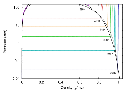
Figure 1: The pressure versus density for various temperatures, including experimental pressure data from NISTnistwater . The solid colored lines indicate the computationally calculated pressure and the dotted colored lines are NIST data points. The solid and dotted black lines represent the theoretical and experimental coexistence curves.

SAFT has been used to construct classical density functionals, which are often used to study the surface tension as a function of temperatureclark2006developing ; gloor2004accurate ; kahl2008modified ; gloor2007prediction ; blas2001examination ; kiselev2006new ; gloor2002saft ; fu2005vapor-liquid-dft ; gross2009density ; yang1994density ; Jaqaman2004 . Such functionals have qualitatively predicted the dependence of surface tension on temperature, but they also overestimate the surface tension by about 50%, and most SAFT-based functionals are unsuited for studying systems that have density variations on a molecular length scale due to the use of a local density approximationgloor2002saft ; clark2006developing ; gloor2007prediction ; gloor2004accurate ; gross2009density ; kahl2008modified ; blas2001examination ; kiselev2006new .

Functionals constructed using a local density approximation fail to satisfy the contact-value theorem, and therefore incorrectly model small hard solutes. The contact-value theorem states that the pressure any fluid exerts on a hard wall interface is proportional to the contact density of the fluidhenderson1979exact :

$$p=n_{c}k_{B}T,$$ (3)

where $n_{c}$ is the contact density, $k_{B}$ is the Boltzmann constant and $T$ is the temperature of the fluid. This leads to the property that the excess chemical potential of a small hard solute is proportional to the solvent-excluded volume:

$$F=nk_{B}TV.$$ (4)

The contact-value theorem is satisfied by classical density functionals in which the only purely local term is the ideal gas contribution to the free energy, and conversely, this theorem is not satisfied by functionals built using a local density approximation.

II Theory and Methods

We construct a classical density functional for water, which reduces in the homogeneous limit to the optimal SAFT model for water found by Clark et al. The Helmholtz free energy is constructed using the first four terms from Equation 2: $F_{\textit{id}}$, $F_{\textit{hs}}$, $F_{\textit{disp}}$ and $F_{\textit{assoc}}$. In the following sections, we will introduce the terms of this functional.

II.1 Ideal gas functional

The first term is the ideal gas free energy functional, which is purely local:

$$F_{id}[n]=k_{B}T\int n(\textbf{r})\left(\ln{\frac{n(\textbf{r})}{n_{Q}}}-1\right)d\textbf{r},$$ (5)

where n(r) is the density of water molecules and $n_{Q}$ is the quantum concentration

$$n_{Q}=\left(\frac{mk_{B}T}{2\pi\hbar^{2}}\right)^{3/2}.$$ (6)

The ideal gas free energy functional on its own satisfies the contact value theorem and its limiting case of small solutes (Equations 3 and 4). These properties are retained by our total functional, since all the remaining terms are purely nonlocal.

II.2 Hard-sphere repulsion

We treat the hard-sphere repulsive interactions using the White Bear version of the Fundamental-Measure Theory (FMT) functional for the hard-sphere fluid roth2002whitebear . FMT functionals are expressed as the integral of the fundamental measures of a fluid, which provide local measures of quantities such as the filling fraction, density of spheres touching a given point and mean curvature. The hard-sphere excess free energy is written as:

$$F_{hs}[n]=k_{B}T\int(\Phi_{1}(\textbf{r})+\Phi_{2}(\textbf{r})+\Phi_{3}(\textbf{r}))d\textbf{r}\;,$$ (7)

with integrands

$$\Phi_{1} =-n_{0}\ln\left(1-n_{3}\right)$$ (8)

$$\Phi_{2} =\frac{n_{1}n_{2}-\mathbf{n}_{V1}\cdot\mathbf{n}_{V2}}{1-n_{3}}$$ (9)

$$\Phi_{3} =(n_{2}^{3}-3n_{2}\mathbf{n}_{V2}\cdot\mathbf{n}_{V2})\frac{n_{3}+(1-n_{3})^{2}\ln(1-n_{3})}{36\pi n_{3}^{2}\left(1-n_{3}\right)^{2}},$$ (10)

where the fundamental measure densities are given by:

$$n_{3}(\textbf{r}) =\int n(\textbf{r}^{\prime})\Theta(\left|\textbf{r}-\textbf{r}^{\prime}\right|-R)d\textbf{r}^{\prime}$$ (11)

$$n_{2}(\textbf{r}) =\int n(\textbf{r}^{\prime})\delta(\left|\textbf{r}-\textbf{r}^{\prime}\right|-R)d\textbf{r}^{\prime}$$ (12)

$$\mathbf{n}_{V2} =\mathbf{\nabla}n_{3}$$ (13)

$$n_{1} =\frac{n_{2}}{4\pi R}$$ (14)

$$\mathbf{n}_{V1} =\frac{\mathbf{n}_{V2}}{4\pi R}$$ (15)

$$n_{0} =\frac{n_{2}}{4\pi R^{2}}.$$ (16)

The density $n_{3}$ is the filling fraction and $n_{2}$ describes the number of spheres touching a given point. For our functional for water, we use the hard-sphere radius of 3.03420 Å, which was found to be optimal by Clark et al.clark2006developing

II.3 Dispersion free energy

The dispersion free energy includes the van der Waals attraction and any orientation-independent interactions. We use a dispersion term based on the SAFT-VR approachgil-villegas-1997-SAFT-VR , which has two free parameters (taken from Clark et alclark2006developing ): an interaction energy $\epsilon_{\textit{d}}$ and a length scale $\lambda_{\textit{d}}R$.

The SAFT-VR dispersion free energy has the form gil-villegas-1997-SAFT-VR

$$F_{\text{disp}}[n] =\int\left(a_{1}(\textbf{r})+\beta a_{2}(\textbf{r})\right)n(\textbf{r})d\textbf{r},$$ (17)

where $a_{1}$ and $a_{2}$ are the first two terms in a high-temperature perturbation expansion and $\beta=1/k_{B}T$. The first term, $a_{1}$, is the mean-field dispersion interaction. The second term, $a_{2}$, describes the effect of fluctuations resulting from compression of the fluid due to the dispersion interaction itself, and is approximated using the local compressibility approximation (LCA), which assumes the energy fluctuation is simply related to the compressibility of a hard-sphere reference fluidbarker1976liquid .

The form of $a_{1}$ and $a_{2}$ for SAFT-VR is given in reference gil-villegas-1997-SAFT-VR , expressed in terms of the filling fraction. In order to apply this form to an inhomogeneous density distribution, we construct an effective local filling fraction for dispersion $\eta_{\textit{d}}$, given by a Gaussian convolution of the density:

$$\eta_{\textit{d}}(\textbf{r}) =\frac{1}{6\sqrt{\pi}\lambda_{\textit{d}}^{3}s_{d}^{3}}\int n(\textbf{r}^{\prime})\exp\left({-\frac{|\textbf{r}-\textbf{r}^{\prime}|^{2}}{2(2\lambda_{\textit{d}}s_{d}R)^{2}}}\right)d\textbf{r}^{\prime}.$$ (18)

This effective filling fraction is used throughout the dispersion functional, and represents a filling fraction averaged over the effective range of the dispersive interaction. Here we have introduced an additional empirical parameter $s_{d}$ which modifies the length scale over which the dispersion interaction is correlated.

II.4 Association free energy

The final attractive energy term is the association term, which accounts for hydrogen bonding. Hydrogen bonds are modeled as four attractive patches (“association sites”) on the surface of the hard sphere. These four sites represent two protons and two electron lone pairs. There is an attractive energy $\epsilon_{\textit{a}}$ when two molecules are oriented such that the proton of one overlaps with the lone pair of the other. The volume over which this interaction occurs is $\kappa_{\textit{a}}$, giving the association term in the free energy two empirical parameters that are fit to the experimental equation of state of water (again, taken from Clark et alclark2006developing ).

The association functional we use is a modified version of Yu and Wuyu2002fmt-dft-inhomogeneous-associating , which includes the effects of density inhomogeneities in the contact value of the correlation function $g^{HS}_{\sigma}$, but is based on the SAFT-HS model, rather than the SAFT-VR modelgil-villegas-1997-SAFT-VR , which is used in the optimal SAFT parametrization for water of Clark et alclark2006developing . Adapting Yu and Wu’s association free energy to SAFT-VR simply involves the addition of a correction term in the correlation function (see Equation 23).

The association functional we use is constructed by using the density $n_{0}(\textbf{r})$, which is the density of hard spheres touching a given point, in the standard SAFT-VR association energygil-villegas-1997-SAFT-VR . The association free energy for our four-site model has the form

$$F_{\text{assoc}}[n] =4k_{B}T\int n_{0}(\textbf{r})\zeta(\textbf{r})\left(\ln X(\textbf{r})-\frac{X(\textbf{r})}{2}+\frac{1}{2}\right)d\textbf{r},$$ (19)

where the factor of $4$ comes from the four association sites per molecule, the functional $X$ is the fraction of association sites not hydrogen-bonded, and $\zeta(\textbf{r})$ is a dimensionless measure of the density inhomogeneity.

$$\zeta(\textbf{r}) =1-\frac{\mathbf{n}_{2V}\cdot\mathbf{n}_{2V}}{n_{2}^{2}}.$$ (20)

The fraction $X$ is determined by the quadratic equation

$$X(\textbf{r}) =\frac{\sqrt{1+8n_{0}(\textbf{r})\zeta(\textbf{r})\Delta(\textbf{r})}-1}{4n_{0}(\textbf{r})\zeta(\textbf{r})\Delta(\textbf{r})},$$ (21)

where the functional $\Delta$ is a measure of hydrogen-bonding probability, given by

$$\Delta(\textbf{r}) =\kappa_{\textit{a}}g^{\textit{SW}}_{\sigma}(\textbf{r})\left(e^{-\beta\epsilon_{\textit{a}}}-1\right)$$ (22)

$$g^{\textit{SW}}_{\sigma}(\textbf{r}) =g^{\textit{HS}}_{\sigma}(\textbf{r})+\frac{1}{4}\beta\left(\frac{\partial a_{1}}{\partial\eta_{\textit{d}}(\textbf{r})}-\frac{\lambda_{\textit{d}}}{3\eta_{\textit{d}}}\frac{\partial a_{1}}{\partial\lambda_{\textit{d}}}\right),$$ (23)

where $g^{\textit{SW}}_{\sigma}$ is the correlation function evaluated at contact for a hard-sphere fluid with a square-well dispersion potential, and $a_{1}$ and $a_{2}$ are the two terms in the dispersion free energy. The correlation function $g^{\textit{SW}}_{\sigma}$ is written as a perturbative correction to the hard-sphere fluid correlation function $g^{\textit{HS}}_{\sigma}$, for which we use the functional of Yu and Wuyu2002fmt-dft-inhomogeneous-associating :

$$g_{\sigma}^{HS} =\frac{1}{1-n_{3}}+\frac{R}{2}\frac{\zeta n_{2}}{(1-n_{3})^{2}}+\frac{R^{2}}{18}\frac{\zeta n_{2}^{2}}{(1-n_{3})^{3}}.$$ (24)

II.5 Determining the empirical parameters

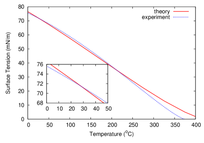
Figure 2: Comparison of Surface tension versus temperature for theoretical and experimental data. The experimental data is taken from NIST.nistwater The length-scaling parameter $s_{d}$ is fit so that the theoretical surface tension will match the experimental surface tension near room temperature.

The majority of the empirical parameters used in our functional are taken from the paper of Clark et al on developing an optimal SAFT model for waterclark2006developing . This SAFT model contains five empirical parameters: the hard-sphere radius, an energy and length scale for the dispersion interaction, and an energy and length scale for the association interaction. In addition to the five empirical parameters of Clark et al, we add a single additional dimensionless parameter $s_{d}$—with a fitted value of 0.353—which determines the length scale over which the density is averaged when computing the dispersion free energy and its derivative. We determine this final parameter by fitting the to the experimental surface tension with the result shown in Figure 2. Because the SAFT model of Clark et al overestimates the critical temperature—which is a common feature of SAFT-based functionals that do not explicitly treat the critical point—we cannot reasonably describe the surface tension at all temperatures, and choose to fit the surface tension at and around room temperature.

III Results and discussion

III.1 One hydrophobic rod

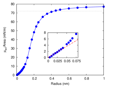
Figure 3: Excess chemical potential per area versus radius for a single hydrophobic rod immersed in water. This should have an asymptote equal to the surface tension at room temperature, and it agrees well with the surface tension in Figure 2. The inset for rods with a very small radius shows the linear relationship expected based on Equation 4.

We begin by studying a single hydrophobic rod immersed in water. In Figure 3 we show the excess chemical potential at room temperature, scaled by the solvent-accessible surface area of the hard rod, plotted as a function of hard-rod radius. We define the hard-rods radius as the radius from which water is excluded. For rods with radius larger than 0.5 nm or so, this reaches a maximum value of 75 mN/m, which is slightly higher than the bulk surface. In the limit of very large rods, this value will decrease and approach the bulk surface value. As seen in the inset of Fig. 3, for rods with very small radius (less than about 0.5 Å) the excess chemical potential is proportional to volume, as required by the contact-value theorem (see Equation 4).

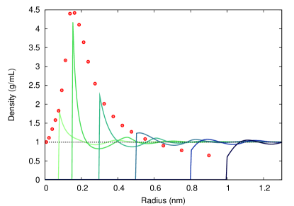
Figure 4: Density profiles for single rods of different radii. The dotted line represents the saturated liquid density and the points represent the expected contact density derived from the contact value theorem and calculated free energy data.

We show in Figure 4 density profiles for different radii rods, as well as the prediction for the contact value of the density as a function of rod radius, as computed from the free energies plotted in Figure 3. The agreement between these curves confirms that our functional satisfies the contact-value theorem and that our minimization is well converged. As expected, as the radius of the rods becomes zero the contact density approaches the bulk density, and as the radius becomes large, the contact density will approach the vapor density.

III.2 Hydrophobic interaction of two rods

We now look at the more interesting problem of two parallel hard rods in water, separated by a distance $d$, as shown in Figure 5. At small separations there is only vapor between the rods, but as the rods are pulled apart, the vapor region expands until a critical separation is reached at which point liquid water fills the region between the rods. Figure 5 shows density profiles before and after this transition for rods of radius 0.6 nm. This critical separation for the transition to liquid depends on the radii of the rods, and is about 0.65 nm for the rods shown in Figure 5. The critical separation will be different for a system where there is attraction between the rods and water. At small separations, the shape of the water around the two rods makes them appear as one solid “stadium”-shaped object (a rectangle with semi-circles on both ends).

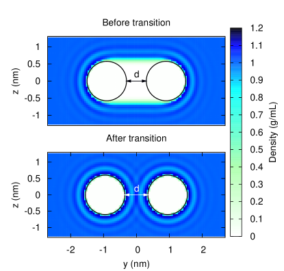
Figure 5: Density profiles illustrating the transition from vapor to liquid water between the rods. The radius is 0.6 nm, the top figure is at a separation of 0.6 nm and the bottom is 0.7 nm. Figure 6 shows the energy for these and other separations.

To understand this critical separation, we consider the free energy in the macroscopic limit, which is given by

$$F=\gamma A+pV.$$ (25)

The first term describes the surface energy and the second term is the work needed to create a cavity of volume $V$. Since the pressure term scales with volume, it can be neglected relative to the surface term provided the length scale is small compared with $\gamma/p$, which is around $20~{}\mu m$, and is much larger than any of the systems we study. For micron-scale rods, the water on the sides of the ‘stadium’ configuration will bow inward between the rods and the density will reduce to vapor near the center point where the rods are closest to each other.

Starting from the surface energy term, we can calculate the free energy per length, which is equal to the circumference multiplied by the surface tension. The force per length is the derivative of this with respect to the separation. The circumference of the stadium-shape is

$$C_{s}=2\pi r+4r+2d$$ (26)

and so the force per length is equal to twice the surface tension.

We plot in Figure 6 the computed free energy of interaction per unit length from our classical density functional (solid lines), as a function of the separation $d$, along with the free energy predicted by our simple macroscopic model (dashed lines). The models agree very well on the force between the two rods at close separations, and have reasonable agreement as to the critical separation for rods greater than 0.5 nm in radius.

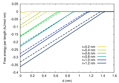
Figure 6: Free energy of interaction (also known as the potential of mean force) versus separation for two hydrophobic rods ranging in radius from 0.2 nm to 1.2 nm. All were arbitrarily offset to zero at large separations for ease of comparison. The transition corresponds to the phase change from vapor to liquid between the rods as pictured in the density profiles in Figure 5.

Walther et alwalther2004hydrophobic studied the interactions between two carbon nanotubes, which are geometrically similar to our hydrophobic rods, using molecular dynamics with the SPC model for water, and a Lennard-Jones potential for the interaction of carbon with water, for nanotubes of diameter 1.25 nm and separations ranging from about 0.3 nm to 1.5 nm. The SPC model underestimates the surface tension of water by about 24%vega2007surface , so we cannot expect this work to provide quantitative agreement with real water. Walther et al observe a drying transition between the two nanotubes, which occurs at a smaller radius than our results suggest. However, when Walther et al disable the attractive interaction between nanotube and water, the drying effect occurs at much longer range, in agreement with our results.

III.3 Hydrophobic interactions of four rods

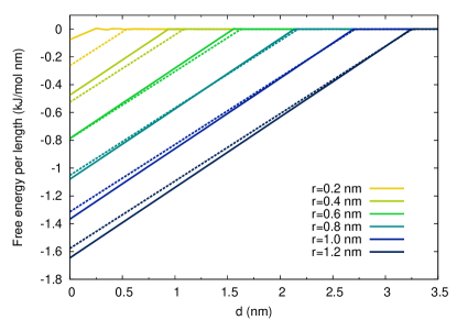
Figure 7: Free energy of interaction versus separation for four hydrophobic rods ranging in radius from 0.2 nm to 1.2 nm. All were arbitrarily offset to zero at large separations. The transition corresponds to the phase change from vapor to liquid between the rods as pictured in the density profiles in Figure 8.

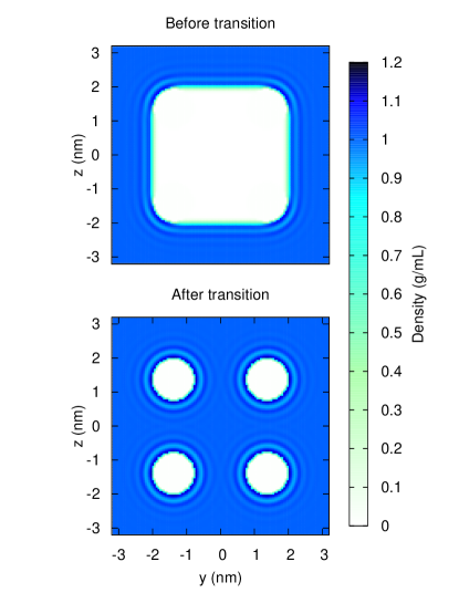
Figure 8: Density profiles illustrating the transition from vapor to liquid water between four rods. The radius is 0.6 nm, the top figure is at a separation of 1.53 nm and the bottom is 1.56 nm. Figure 7 shows the energy for these and other separations.

We go on to study four parallel hard rods, as examined by Lum, Chandler and Weeks in their classic paper on hydrophobicity at small and large length scales lum1999hydrophobicity . As in the case of two rods—and as predicted by Lum et al—we observe a drying transition, as seen the density plot shown in Figure 8. In Figure 7, we plot the free energy of interaction together with the macroscopic approximation, and find good agreement for rods larger than 0.5 nm in radius. This free energy plot is qualitatively similar to that predicted by the LCW theory lum1999hydrophobicity , with the difference that we find no significant barrier to the association of four rods.

III.4 Hydration energy of hard-sphere solutes

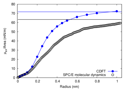
Figure 9: Excess chemical potential per area versus radius for a single hydrophobic sphere immersed in water. This should have an asymptote equal to the surface tension at room temperature, and it agrees well with the surface tension in Figure 2. Results from a simulation of SPC/E water huang2001shs are shown as circles. The horizontal lines show the experimental and SPC/E bulk surface tension for water at standard atmospheric temperature and pressure.

A common model of hydrophobic solutes is the hard-sphere solute, which is the simplest possible solute, and serves as a test case for understanding of hydrophobic solutes in watersedlmeier2011entropy . As in the single rod, we begin by examining the ratio of the excess chemical potential of the cavity system to the solvent-accessible surface area (Figure 9). This effective surface tension surpasses the bulk surface tension at a radius of almost 1 nm, and at large radius will drop to the bulk value. As with the single rod, we see the analytically correct behavior in the limit of small solutes. For comparison, we plot the free energy calculated using a molecular dynamics simulation of SPC/E waterhuang2001shs . The agreement is quite good, apart from the issue that the SPC/E model for water significantly underestimates the surface bulk tension of water at room temperaturevega2007surface .

Figure 10 shows the density profile for several hard sphere radii, plotted together with the results of the same SPC/E molecular dynamics simulation shown in Figure 9huang2001shs . The agreement with simulation is quite reasonable. The largest disagreement involves the density at contact, which according to the contact value theorem cannot agree, since the free energies do not agree.

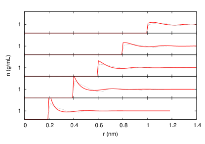
Figure 10: Density profiles around hard-sphere solutes of different radii. Predictions from our classical density-functional theory are in solid red, while the dotted line shows the result of a molecular dynamics simulation of SPC/E water huang2001shs .

IV Conclusion

We have developed a classical density functional for water that combines SAFT with the fundamental-measure theory for hard spheres, using one additional empirical parameter beyond those in the SAFT equation of state, which is used to match the experimental surface tension. This functional does not make a local density approximation, and therefore correctly models water at both small and large length scales. In addition, like all FMT functionals, this functional is expressed entirely in terms of convolutions of the density, which makes it efficient to compute and minimize.

We apply this functional to the case of hard hydrophobic rods and spheres in water. For systems of two or four hydrophobic rods surrounded by water, we see a transition from a vapor-filled state a liquid-filled state. A simple model treatment for the critical separation for this transition works well for rods with diameters larger than 1 nm. In the case of spherical solutes, we find good agreement with SPC/E simulations.

References

- (1) R. Car and M. Parrinello, Phys. Rev. Lett. 55, 2471 (Nov 1985)
- (2) J. C. Grossman, E. Schwegler, E. W. Draeger, F. Gygi, and G. Galli, The Journal of Chemical Physics 120, 300 (2004), http://link.aip.org/link/?JCP/120/300/1
- (3) T. Lewis, B. Winter, A. C. Stern, M. D. Baer, C. J. Mundy, D. J. Tobias, and J. C. Hemminger, J. Phys. Chem. C 115, 21183 (2011)
- (4) S. Yoo, X. Zeng, and S. Xantheas, The Journal of chemical physics 130, 221102 (2009)
- (5) I. Lin, A. Seitsonen, M. Coutinho-Neto, I. Tavernelli, and U. Rothlisberger, The Journal of Physical Chemistry B 113, 1127 (2009)
- (6) J. Wang, G. Roma´ n Pe´ rez, J. Soler, E. Artacho, and M. Ferna´ ndez Serra, Journal of Chemical Physics 134, 24516 (2011)
- (7) A. Møgelhøj, A. Kelkkanen, K. Wikfeldt, J. Schiøtz, J. Mortensen, L. Pettersson, B. Lundqvist, K. Jacobsen, A. Nilsson, and J. Nørskov, The Journal of Physical Chemistry B(2011)
- (8) R. Jonchiere, A. Seitsonen, G. Ferlat, A. Saitta, and R. Vuilleumier, The Journal of chemical physics 135, 154503 (2011)
- (9) J. Morrone and R. Car, Physical review letters 101, 17801 (2008)
- (10) K. Lum, D. Chandler, and J. Weeks, The Journal of Physical Chemistry B 103, 4570 (1999)
- (11) W. M. Latimer, K. S. Pitzer, and C. M. Slansky, The Journal of Chemical Physics 7, 108 (1939), http://link.aip.org/link/?JCP/7/108/1
- (12) A. A. Rashin and B. Honig, Journal of Physical Chemistry 89, 5588 (1985), ISSN 0022-3654
- (13) C.-G. Zhan, J. Bentley, and D. M. Chipman, J. Chem. Phys. 108, 177 (1998)
- (14) C.-P. Hsu, M. Head-Gordon, and T. Head-Gordon, J. Chem. Phys. 111, 9700 (December 1999)
- (15) A. Hildebrandt, R. Blossey, S. Rjasanow, O. Kohlbacher, and H.-P. Lenhof, Physical Review Letters 93, 108104 (2004), http://link.aps.org/abstract/PRL/v93/e108104
- (16) A. Hildebrandt, R. Blossey, S. Rjasanow, O. Kohlbacher, and H.-P. Lenhof, Bioinformatics 23, e99 (2007), http://bioinformatics.oxfordjournals.org/cgi/reprint/23/2/e99.pdf, http://bioinformatics.oxfordjournals.org/cgi/content/abstract/23/2/e99
- (17) C. Ebner, W. Saam, and D. Stroud, Physical Review A 14, 2264 (1976)
- (18) N. Mermin, Physical Review 137, 1441 (1965)
- (19) P. Hohenberg and W. Kohn, Physical Review 136, B864 (1964)
- (20) W. A. Curtin and N. W. Ashcroft, Phys. Rev. A 32, 2909 (Nov 1985)
- (21) Y. Rosenfeld, Phys. Rev. Lett. 63, 980 (Aug 1989)
- (22) Y. Rosenfeld, J. Chem. Phys. 98, 8126 (May 1993)
- (23) Y. Rosenfeld, M. Schmidt, H. Löwen, and P. Tarazona, Phys. Rev. E 55, 4245 (Apr 1997)
- (24) P. Tarazona and Y. Rosenfeld, Phys. Rev. E 55, R4873 (May 1997)
- (25) P. Tarazona, Phys. Rev. Lett. 84, 694 (Jan 2000)
- (26) R. Roth, R. Evans, A. Lang, and G. Kahl, Journal of Physics: Condensed Matter 14, 12063 (2002)
- (27) K. Ding, D. Chandler, S. J. Smithline, and A. D. J. Haymet, Phys. Rev. Lett. 59, 1698 (Oct 1987)
- (28) B. Yang, D. Sullivan, B. Tjipto-Margo, and C. Gray, Molecular Physics 76, 709 (June 1992)
- (29) B. Yang, D. Sullivan, and C. Gray, Journal of Physics: Condensed Matter 6, 4823 (1994)
- (30) G. Gloor, F. Blas, E. del Rio, E. de Miguel, and G. Jackson, Fluid phase equilibria 194, 521 (2002)
- (31) G. Gloor, G. Jackson, F. Blas, E. Del Río, and E. de Miguel, The Journal of chemical physics 121, 12740 (2004)
- (32) G. Gloor, G. Jackson, F. Blas, E. del Río, and E. de Miguel, The Journal of Physical Chemistry C 111, 15513 (2007)
- (33) K. Jaqaman, K. Tuncay, and P. J. Ortoleva, J. Chem. Phys. 120, 926 (2004)
- (34) G. Clark, A. Haslam, A. Galindo, and G. Jackson, Molecular physics 104, 3561 (2006)
- (35) G. N. Chuev and V. F. Sokolov, Journal of Physical Chemistry B 110, 18496 (2006)
- (36) J. Lischner and T. Arias, The Journal of Physical Chemistry B 114, 1946 (2010)
- (37) D. Fu and J. Wu, Ind. Eng. Chem. Res 44, 1120 (2005)
- (38) S. Kiselev and J. Ely, Chemical Engineering Science 61, 5107 (2006), ISSN 0009-2509
- (39) F. Blas, E. Del Río, E. De Miguel, and G. Jackson, Molecular Physics 99, 1851 (2001)
- (40) Y. X. Yu and J. Wu, The Journal of Chemical Physics 116, 7094 (2002)
- (41) E. A. Müller and K. E. Gubbins, Industrial & engineering chemistry research 40, 2193 (2001)
- (42) J. Gross, The Journal of chemical physics 131, 204705 (2009)
- (43) H. Kahl and J. Winkelmann, Fluid Phase Equilibria 270, 50 (2008)
- (44) M. S. Wertheim, Journal of statistical physics 35, 19 (1984)
- (45) M. S. Wertheim, Journal of statistical physics 35, 35 (1984)
- (46) M. S. Wertheim, Journal of statistical physics 42, 459 (1986)
- (47) M. S. Wertheim, Journal of statistical physics 42, 477 (1986)
- (48) A. Gil-Villegas, A. Galindo, P. Whitehead, S. Mills, G. Jackson, and A. Burgess, The Journal of Chemical Physics 106, 4168 (1997)
- (49) E. W. Lemmon, M. O. McLinden, and D. G. Friend, “Nist chemistry webbook, nist standard reference database number 69,” (National Institute of Standards and Technology, Gaithersburg MD, 20899, 2010) Chap. Thermophysical Properties of Fluid Systems, http://webbook.nist.gov, (retrieved December 15, 2010)
- (50) D. Henderson, L. Blum, and J. Lebowitz, Journal of Electroanalytical Chemistry and Interfacial Electrochemistry 102, 315 (1979)
- (51) J. Barker and D. Henderson, Reviews of Modern Physics 48, 587 (1976)
- (52) J. Walther, R. Jaffe, E. Kotsalis, T. Werder, T. Halicioglu, and P. Koumoutsakos, Carbon 42, 1185 (2004)
- (53) C. Vega and E. De Miguel, The Journal of chemical physics 126, 154707 (2007)
- (54) D. Huang, P. Geissler, and D. Chandler, Journal of Physical Chemistry B 105, 6704 (2001)
- (55) F. Sedlmeier, D. Horinek, and R. Netz, The Journal of chemical physics 134, 055105 (2011)