On correlation between protein secondary structure,
backbone bond angles, and side-chain orientations

Abstract

We investigate the fine structure of the $sp3$ hybridized covalent bond geometry that governs the tetrahedral architecture around the central C_α carbon of a protein backbone, and for this we develop new visualization techniques to analyze high resolution X-ray structures in Protein Data Bank. We observe that there is a correlation between the deformations of the ideal tetrahedral symmetry and the local secondary structure of the protein. We propose a universal coarse grained energy function to describe the ensuing side-chain geometry in terms of the C_β carbon orientations. The energy function can model the side-chain geometry with a sub-atomic precision. As an example we construct the C_α-C_β structure of HP35 chicken villin headpiece. We obtain a configuration that deviates less than 0.4 Ȧ in root-mean-square distance from the experimental X-ray structure.

I I: Introduction

Protein structure validation is based on various well tested and broadly accepted stereochemical paradigms. Methods such as MolProbity mol and Procheck pro and many others help crystallographers to find and fix potential problems during fitting and refinement. Stereochemical assumptions are also instrumental to structure prediction packages such as Rosetta and I-Tasser ros . Likewise, they form the foundation for parameter determination in force fields such as Charmm and Amber nat that aim to describe protein dynamics at atomic scale.

One of the paradigms is the transfersability assumption. It states that stereochemical restraints are universal and independent of the environment. Among its consequences are that the covalent bond geometry around the backbone C_α should seize a very precise tetrahedral $sp3$ hybridized shape. For example, the backbone

$$\tau_{NC}\ \equiv\ (N-C_{\alpha}-C)$$

bond angle should oscillate around a computable average value that depends only on the covalent bonds between the C_α and the N, C, H and C_β atoms in the trans-peptide group. In particular, at least to to the leading order its value should not depend on the character of the secondary structure environment. Standard molecular dynamics force fields explicitly assume this to be the case. These force fields are based on a harmonic approximation where the bond angles $\kappa$ oscillate with energy nat

$$E_{bond}=\sum_{\rm bonds}\omega_{\kappa}(\kappa-\kappa_{0})^{2}$$ (1)

Here $\omega_{\kappa}$ and $\kappa_{0}$ are parameters that are in general amino acid dependent. But these parameters are presumed to be independent of the geometry of the surrounding secondary structure. Instead, they are supposed to predict the local secondary structure environment.

The enormous success that has been enjoyed by the validation methods and structure prediction programs in resolving close to 80.000 crystallographic protein structures that are presently in Protein Data Bank (PDB) struc is a clear manifestation that the various paradigms are valid to a good precision. However, with the advent of third-generation synchrotron sources of X-rays, there is now a small but rapidly expanding number of protein structures that are resolved with an ultrahigh sub-Angström resolution. The present, third-generation X-ray synchrotron sources such as ESRF in Grenoble and PETRA at DESY in Hamburg can already produce photons with wavelengths as short as 10 pico-meters. Thus it is in principle possible to obtain three dimensional protein structures with a comparable resolution. The next-generation sources of high brilliance X-ray beams such as the European X-Ray Free Electron Laser at DESY, will push protein X-ray crystallography to its extreme. These future experimental facilities can reach both ultra-high spatial and temporal resolutions, with a fully coherent peak brightness that is many orders of magnitude higher than what can be obtained with the present third-generation synchrotron sources. The on-going experimental revolution in combination with the ever expanding need of higher precision for example in the study of protein-protein interactions, enzyme catalysis and search of causes for protein misfolding related diseases, are good incentives for us to scrutinize the level of precision in some of the paradigm assumptions on protein backbone geometry. And, if need be, to try and develop new theoretical concepts that aim to describe proteins at a precision that matches the highest present and near future experimental standards, in revealing the finer structures of folded proteins.

In fact, ab initio quantum mechanical calculations sch and empirical studies krp1 -tou of protein backbone geometry have already disclosed that the backbone bond angle $\tau_{NC}\equiv$ (N-C_α-C) about the C_α carbons might oscillate quite substantially. The range of variations can be as large as 8.8^o krp2 . This corresponds to a shift of $\sim\!0.6$ Å  in the relative positioning of two consecutive C_α carbons. A deviation of this size from the ideal value can be subjected to experimental scrutiny in X-ray experiments that reach sub-Ångström resolution. Indeed, on the basis of existing data the authors krp1 -tou have already reported that the deviations in the values of the $\tau_{NC}$ angle are systematic, and in particular that these deviations reflect the local secondary structure.

The $\tau_{NC}$ angles are primarily affected by the backbone. As such, their values relate directly to the two standard Ramachandran angles, that form the basis for structure validation. As a consequence, the literature sch -tou has until now mainly concentrated on the effects that potential deviations of $\tau_{NC}$ from ideality have on the backbone geometry. Here we extend this analysis to the side-chains: The fluctuations in the lengths of the covalent bonds in the C_α tetrahedron are no more than around 0.1 Å  which is much less than the potential $\sim\!0.6$ Å  shift in the relative positioning of two consecutive C_α carbons, due to $\tau_{NC}$ fluctuations krp1 -tou . This proposes that any deviation of $\tau_{NC}$ from its ideal value inevitably propagates to the side-chain dependent $\tau_{N\beta}\equiv$ (N-C_α-C_β) and $\tau_{C\beta}\equiv$ (C-C_α-C_β) bond angles, and this should lead to observable effects in the angular positions of the side-chain C_β atoms.

In this article we first analyze PDB data to find whether there are experimental variations in the tetrahedral angles around the C_α. In particular, we extend the analysis of krp1 -tou to study correlations between the side-chain dependent angles $\tau_{N\beta}$ and $\tau_{C\beta}$ that determine the C_β orientations, and the local secondary structure of the backbone. Since the side-chain atom positions are not easily described in terms of the backbone Ramachandran angles, we start by developing new visualization tools. In line with krp1 -tou we observe that the local secondary structure has a systematic effect on the relative tetrahedral position of the C_β carbon. We then proceed to utilize our visualization tools to develop theoretical arguments. We propose a coarse-grained framework that computes how the observed direction of the C_β evolves along the backbone. In particular, we argue that the direction of the C_β can be computed from the soliton solution of a discrete nonlinear Schrödinger (DNLS) equation. The DNLS soliton already shares a remarkable history with protein research dnls . Both the DNLS equation and its soliton solution were first introduced by Davydov to describe the propagation of energy along $\alpha$-helices davy . He also proposed that since the propagation leads to a local deformation of the protein shape, a trapped soliton is a natural cause for the protein to fold. Here we first argue on general grounds that the DNLS soliton solution can be utilized to determine the secondary structure dependence in the relative direction of the C_β atoms along the backbone. We then consider an explicit example to illustrate our general arguments. The example we consider is the 35-residue subdomain of the villin headpiece with PDB code 1YRF. It is a paradigm protein that has been studied widely in theoretical approaches to protein folding.

II II: Visualization of the C_α tetrahedron

We start by visual analysis of crystallographic protein data in PDB. The goal is to reveal any secondary structure dependence in the values of $\tau_{NC}$, and in the adjacent

$$\tau_{N\beta}\ \equiv\ (N-C_{\alpha}-C_{\beta})$$

and

$$\tau_{C\beta}\ \equiv\ (C-C_{\alpha}-C_{\beta})$$

bond angles. In order to minimize any bias, we inspect several subsets of PDB. These include the canonical one that comprises all PDB configurations with resolution 2.0 Ȧ or better, and its two subsets with resolution better than 1.5 Ȧ, and better than 1.0 Ȧ. We also inspect a subset of the 2.0 Ȧ set that contains only those proteins that have less than 30$\%$ sequence similarity. Our conclusions are independent of the data set, and for illustrative purposes we here use the canonical 2.0 Ȧ set. There are presently over 30.000 such entries in PDB.

The Ramachandran angles are defined in terms of the backbone amide planes. As such they are not the most convenient ones for describing the side-chain geometry. Since both $\tau_{N\beta}$ and $\tau_{C\beta}$ relate to the side-chain geometry, we prefer to follow dff and describe the folded protein structure in terms of the geometrically determined backbone discrete Frenet frames (DFF). These frames govern the entire backbone neighborhood, including the side-chains. But their construction involves only the C_α coordinates ${\bf r}_{i}$ where $i=1,...,N$ label the residues. As such, these frames then give a manifestly N, C_β and C independent, purely geometric description of the tetrahedral $sp3$ neighborhood of the C_α atoms.

The backbone tangent vectors are

$$\mathbf{t}_{i}=\frac{{\bf r}_{i+1}-{\bf r}_{i}}{|{\bf r}_{i+1}-{\bf r}_{i}|}$$ (2)

The unit binormal vectors are

$$\mathbf{b}_{i}=\frac{{\mathbf{t}}_{i-1}-{\mathbf{t}}_{i}}{|{\mathbf{t}}_{i-1}-{\mathbf{t}}_{i}|}$$ (3)

The unit normal vectors

$$\mathbf{n}_{i}=\mathbf{b}_{i}\times\mathbf{t}_{i}$$ (4)

The orthogonal triplets ($\mathbf{n}_{i},\mathbf{b}_{i},\mathbf{t}_{i}$) determine the discrete Frenet frame at each of the positions $\mathbf{r}_{i}$ of the C_α carbons. Note that if the tangent vectors and the distances between the C_α are known, we can reconstruct the entire C_α backbone using

$$\mathbf{r}_{k}=\sum_{i=1}^{k-1}|\mathbf{r}_{i+1}-\mathbf{r}_{i}|\cdot\mathbf{t}_{i}$$ (5)

For the initial condition we can utilize Galilean invariance to take $\mathbf{r}_{1}=0$, and $\mathbf{t}_{1}$ to point into the direction of the positive $z$-axis. In particular, (5) does not involve the vectors $\mathbf{n}_{i}$ and $\mathbf{b}_{i}$.

We introduce the backbone bond angles

$$\cos\kappa_{i+1}\ \equiv\ \cos\kappa_{i+1,i}={\bf t}_{i+1}\cdot{\bf t}_{i}$$ (6)

and the backbone torsion angles

$$\cos\tau_{i+1}\ \equiv\ \cos\tau_{i+1,i}={\bf b}_{i+1}\cdot{\bf b}_{i}$$ (7)

Note that both angles are manifestly independent of the N, C_β and C atoms that are covalently bonded to the C_α atoms, in this sense they provide an unbiased set of coordinates for describing the positions of these atoms. If these angles are known, we can use

$$\left(\begin{matrix}{\bf n}_{i+1}\\ {\bf b}_{i+1}\\ {\bf t}_{i+1}\end{matrix}\right)=\left(\begin{matrix}\cos\kappa\cos\tau&\cos\kappa\sin\tau&-\sin\kappa\\ -\sin\tau&\cos\tau&0\\ \sin\kappa\cos\tau&\sin\kappa\sin\tau&\cos\kappa\end{matrix}\right)_{\hskip-2.84544pti+1,i}\left(\begin{matrix}{\bf n}_{i}\\ {\bf b}_{i}\\ {\bf t}_{i}\end{matrix}\right)$$

$$\equiv\ {\mathcal{R}}_{i+1,i}\left(\begin{matrix}{\bf n}_{i}\\ {\bf b}_{i}\\ {\bf t}_{i}\end{matrix}\right)$$ (8)

to iteratively construct the Frenet frame at position $i+i$ from the frame at position $i$. Once we have all the frames, we can proceed to construct the entire backbone using (5).

The bond and torsion angles have a natural interpretation in terms of the canonical latitude and longitude angles of a two-sphere $\mathbb{S}^{2}$. In the sequel we find it useful to extend the range of $\kappa_{i}$ to $[-\pi,\pi]\ mod(2\pi)$. But we introduce no change in the range of $\tau_{i}\in[-\pi,\pi]\ mod(2\pi)$. We compensate for this two-fold covering of $\mathbb{S}^{2}$ by the following discrete $\mathbb{Z}_{2}$ symmetry

$$\begin{matrix}\kappa_{k}\ \to\ -\kappa_{k}\ \ \ {\rm for~{}all~{}}\ k\geq i\\ \hskip-54.06006pt\tau_{i}\ \to\ \tau_{i}-\pi\end{matrix}$$ (9)

It inverts the directions of the vectors $\mathbf{n}_{i}$ and $\mathbf{b}_{i}$ but has no effect on the $\mathbf{t}_{i}$ and consequently leaves the backbone intact. For details we refer to dff .

We use the discrete Frenet frames to display each atom in the way, how the atom is seen on the surface of a sphere that surrounds an imaginary observer who roller-coasts the backbone along the C_α atoms, so that the gaze direction is always fixed towards the next C_α and with local orientation determined by the DFF frames dff .

In Figure 1 we show the statistical angular distribution of the backbone N and C atoms, and in Figure 2 we show the same for the side-chain C_β atoms in our PDB data set as seen by the Frenet frame observer who moves through all the proteins in our data set. The sphere is centered at the C_α, and its radius coincides with the length of the (approximatively constant) covalent bond. We take the vector $\bf t$ that points towards the next C_α to be in the direction of the positive $z$-axis, towards the north-pole of the sphere. With $\mathbf{n}$ in the direction of positive $x$-axis we have a right-handed Cartesian coordinate system. We introduce the canonical spherical coordinates ($\theta,\varphi$) to describe the distributions. The angle $\theta\in[0,\pi]$ measures latitude from the positive $z$-axis, hence it describes the distribution of the bond angles $\kappa_{i}$. The angle $\varphi\in[-\pi,\pi]$ measures longitude in a counterclockwise direction from the $x$-axis i.e. from the direction of $\mathbf{n}$ towards that of $\mathbf{b}$, with $\varphi=0$ at the $x$-axis. Consequently it describes the distribution of the torsion angles $\tau_{i}$.

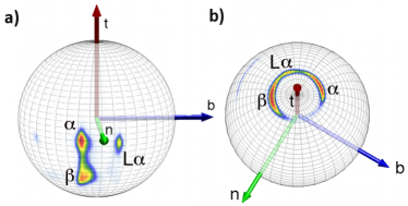
Figure 1: (Color online) The directions of a) backbone N-atoms and b) backbone C-atoms as seen by a Frenet frame observer located at the C_α carbon which is at the center of the sphere. In a) the smaller, more point-like direction of backbone N atoms corresponds to the L-$\alpha$ Ramachandran region. The larger region forms a segment of the great circle $\varphi\approx-15^{\mathrm{o}}$. Loops interpolate latitudinally between $\alpha$-helices and $\beta$-sheets. In b) the directions of backbone C form a segment of a small circle around $z$-axis, with $\theta\approx 20^{\mathrm{o}}$.

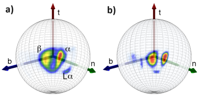
Figure 2: (Color online) The distribution of the C_β directions in the Frenet frame. In a) we have all amino acids (including proline but excluding glycine that has no C_β). In b) we show only proline. Comparison between a) and b) exemplifies how the C_β direction can depend on the individual amino acid. We have chosen proline in b) as it is particularly interesting due to the way how it appears in Figure 3b).

We find that in the Frenet frame coordinate system, the N and C oscillations shown in Figures 1a) and 1b) are fully separated into the locally orthogonal $\theta$ and $\varphi$ directions, respectively. This would certainly not be the case in a generic coordinate system. Furthermore, secondary structures such as $\alpha$-helices, $\beta$-sheets, loops and left-handed $\alpha$-regions are all clearly identifiable in Figures 1. Figure 2a) reveals how the N and C oscillations of Figure 1, through the covalent bonds that form the $sp3$ tetrahedron around C_α, combine into a horseshoe (annulus) shaped nutation of C_β. As visible in the Figure, this nutation reflects the local secondary structure environment in an equally systematic manner as Figures 1.

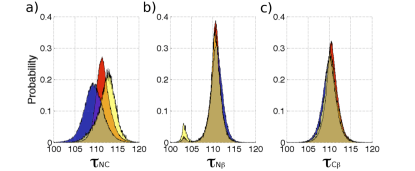
Figure 3: (Color online) The normalized probability density angular distribution of the a) $\tau_{NC}$, b) $\tau_{N\beta}$ and c) $\tau_{C\beta}$ angles in degrees, with $\alpha$-helices in red (grey), $\beta$-strands in blue (dark grey), and 3/10 helices in yellow. The secondary peak in b) is due to cis-peptide prolines. Only in Figure a) are the different secondary structures visibly separated from each other. In Figures b) and c) they are practically fully overlapping, the only notable effect is the somewhat higher propensity of 3/10 helices in connection of cis-peptide prolines.

The pattern of angular separation in the N and C oscillations in Figure 1 reveals that the underlying ideal tetrahedral covalent symmetry around C_α is not transferable along the protein backbone krp1 -tou .

We proceed to Figures 3 a)-c) where we plot the tetrahedral bond angles $\tau_{NC}$, $\tau_{C\beta}$ and $\tau_{N\beta}$ jointly for the $\alpha$-helices, $\beta$-strands and $3/10$-helices. As in figure 1 the loops interpolate continuously between these regular secondary structures. The Figure 3a) clearly reveals that at the level of the $\tau_{NC}$ angle the transferability of the tetrahedral symmetry is absent in a systematic and secondary structure dependent manner. But neither $\tau_{C\beta}$ nor $\tau_{N\beta}$ show any sign whatsoever of secondary structure dependence. The distributions are practically the same, independently of the secondary structure. (The isolated small peak in Figure 3b) is due to proline cis-peptide groups.)

As such, the distribution in both Figures 3b) and 3c) is what we would expect in the case of ideal, transferable $sp3$ tetrahedral symmetry. In each Figure the average value is around $111^{\rm o}$ and there are secondary structure independent fluctuations that are in line with quantum mechanical estimates and sch and empirical studies krp1 -tou . But the fact that $\tau_{NC}$ in Figure 3a) displays clearly visible and systematic secondary structure dependence makes it plain and clear that the paradigm of transferable tetrahedral covalent symmetry around the C_α carbon is absent. Furthermore, the way how transferability becomes violated reflects the wider secondary structure environment of the amino acid along the protein backbone.

Since the deviation from the ideal tetrahedral symmetry is organized in the same way how the proteins are folded, these two must share a common origin. But we do not have any physical explanation why the lack of ideal symmetry is only visible in $\tau_{NC}$. We suspect this has to do with existing experimental refinement methods, the way how refinement tension is distributed between the backbone and side-chains. The high resolution crystallographic data which becomes available in future third and fourth generation experiments should help to clarify this.

III III: Solitons and side-chains

Any molecular dynamics approach to protein folding that we are familiar with, utilizes the harmonic approximation (1) for bond and torsion angles. Here $\kappa_{0}$ is in general amino acid dependent but secondary structure independent equilibrium value of the bond angle. But from Figure 3a) we observe, that for the $\tau_{NC}$ angle there are three different major equilibrium values. These equilibrium bond angle values are amino acid independent, but do depend in a nontrivial manner on the local secondary structure: The three peaks in Figure 3a) correspond to the $\alpha$-helix, $\beta$-strand, and $3/10$-helix while for a loop the values of the corresponding equilibrium $\kappa_{0}$ interpolates between these three ground state values. Since each of these secondary structures are characterized by a different equilibrium value of bond angle $\kappa$, to the leading order we may take $\kappa_{0}$ to be a function of $\kappa$. By expanding to leading order we get

$$\kappa_{0}\to\kappa_{0}(\kappa)\ \approx\ \kappa^{(0)}_{0}+\kappa^{(1)}_{0}\cdot\kappa+\kappa^{(2)}_{0}\cdot\kappa^{2}+\mathcal{O}(\kappa^{3})$$

where the $\kappa^{(i)}$ are independent of the local value of $\kappa$. The first two terms simply renormalize the values of $\omega_{\kappa}$ and $\kappa_{0}$ in (1). But the third term is conceptually different. It introduces an anharmonic correction. We conclude that after redefinitions of the parameters, in the leading order the potential obtains the functional form

$$E_{bond}\ \sim\ q\cdot(\kappa^{2}-m^{2})^{2}$$ (10)

We argue that based on the Figure 3a), the anharmonic corrections are already visible in the existing high resolution X-ray data. In order to answer the theoretical challenge that this poses, we propose to improve existing MD force fields, to account for the anharmonic corrections in the bond angle contribution.

III.1 A: Backbone energy

The presence of an anharmonic correction in the bond angle energy has important implications to the way how proteins fold. For this we start with a simple example. We consider the anharmonic potential (10) in the presence of a single coordinate $x$ on a line. The Newton’s equation is

$$m\ddot{x}=-\frac{dV}{dx}$$

We take the potential to have the form

$$V(x)=\frac{\sigma}{4}\hskip 0.85358pt\,(x+b)^{2}\cdot(x-a)^{2}$$ (11)

We introduce

$$c=-\frac{1}{2}(b+a)$$

and define

$$y=x-\frac{1}{2}(a-b)$$

to arrive at the equation of motion

$$\ddot{y}=-\frac{\sigma}{m}{y}({y}^{2}-c^{2})$$

which is essentially the continuum nonlinear Schrödinger equation (NLSE) dnls , davy Note that the potential has the symmetric form (10). This equation is solved by

$${y}(t)\ =\ c\cdot\tanh[\,c\,\sqrt{\frac{\sigma}{2m}}(t-t_{0})]$$

$$\Rightarrow\ x(t)\ =\ y(t)+\frac{1}{2}(a-b)$$

$$=\ -\,\frac{b\cdot e^{c\,\sqrt{\frac{\sigma}{2m}}(t-t_{0})}\ -\ a\cdot e^{-c\,\sqrt{\frac{\sigma}{2m}}(t-t_{0})}}{\cosh[c\,\sqrt{\frac{\sigma}{2m}}(t-t_{0})]}$$ (12)

This is the hallmark NLSE soliton configuration, so called dark soliton solution of the NLSE equation. It interpolates between the two uniform ground states at $x=a$ and $x=-b$ when $t\to\pm\infty$. The parameters $a$, $b$, $t_{0}$ and the combination

$$c\,\sqrt{\frac{\sigma}{2m}}$$

are the canonical ones that characterize the asymptotic values of $x(t)$ i.e. minima of the potential, and the size and location of the soliton.

For finite $t$ the soliton (12) describes a configuration with an energy above the uniform ground state $x\equiv a$ (or $x\equiv b$). Nevertheless, it can not decay into $x\equiv a$ (or $x\equiv b$) through any kind of continuous finite energy transformation. In particular, a soliton configuration such as (12) can not be obtained from any approach that only accounts for perturbations that describe small localized fluctuations around the uniform background ground state.

In oma2 -and1 , it has been shown that the soliton profile (12) can be used to describe loops in folded proteins. For this one merges general geometric arguments with the concept of universality widom -fisher , to arrive at the following simplified, coarse-grained energy function for the backbone bond and torsion angles oma1 , ulf ,

$$E=-\sum\limits_{i=1}^{N-1}2\,\kappa_{i+1}\kappa_{i}+\sum\limits_{i=1}^{N}\biggl{\{}2\kappa_{i}^{2}+q\cdot(\kappa_{i}^{2}-m^{2})^{2}$$

$$\left.+\frac{d_{\tau}}{2}\,\kappa_{i}^{2}\tau_{i}^{2}-{b_{\tau}}\kappa_{i}^{2}\tau_{i}-a_{\tau}\tau_{i}+\frac{c_{\tau}}{2}\tau^{2}_{i}\right\}$$ (13)

where $\kappa_{i}$ and $\tau_{i}$ are the backbone bond and torsion angles (6), (7). Unlike force fields in molecular dynamics, the energy function (13) does not purport to explain the fine details of the atomic level mechanisms that give rise to protein folding. Instead, in line with general principles of effective Landau-Lifschitz theories it describes the properties of a folded protein backbone in terms of universal physical arguments. Indeed, according to the concept of universality widom -fisher the energy function (13) can be viewed as the universal long distance limit that emerges from any atomic level energy function when the internal energy is coarse-grained to include only the backbone bond and torsion angles.

In order to construct the soliton solution, we start by introducing the $\tau$-equation of motion

$$\frac{\partial E}{\partial\tau_{i}}=d_{\tau}\kappa_{i}^{2}\tau_{i}-b_{\tau}\kappa_{i}^{2}-a_{\tau}+c_{\tau}\tau_{i}=0$$

$$\Rightarrow\ \tau_{i}[\kappa]=\frac{a_{\tau}+b_{\tau}\kappa_{i}^{2}}{c_{\tau}+d_{\tau}\kappa^{2}_{i}}$$ (14)

Notice that even though there are four parameters in (14) one of them, the overall scale, drops out. We then use (14) to eliminate the torsion angles, so that the energy for the bond angles becomes

$$E[\kappa]=-\sum\limits_{i=1}^{N-1}2\,\kappa_{i+1}\kappa_{i}+\sum\limits_{i=1}^{N}2\kappa_{i}^{2}+V[\kappa_{i}]$$ (15)

where

$$V[\kappa]=-\left(\frac{b_{\tau}c_{\tau}-a_{\tau}d_{\tau}}{d_{\tau}}\right)\cdot\frac{1}{c_{\tau}+d_{\tau}\kappa^{2}}$$

$$-\left(\frac{b_{\tau}^{2}+8qm^{2}}{2b_{\tau}}\right)\cdot\kappa^{2}+q\cdot\kappa^{4}$$ (16)

Because the first term contains $\kappa$ in the denominator, its variation with $\kappa$ is not that pronounced as the variation of the other two terms, which are proportional to the second and the fourth power of $\kappa$, respectively. Moreover, because $|\kappa|>1$ radian for proteins, it turns out that the first term is small in value compared to the other terms. The second and third terms have then the functional form of the double well potential (10).

In applications to folded proteins the parameters values are such, that in the energy ground state both $\kappa$ and $\tau$ acquire a non-vanishing value. In particular, since the functional form of (16) is similar to (10), (11) we can expect that there are soliton solutions:

Geometrically, a uniform constant value of the bond and torsion angles describes regular protein secondary structures. For example, the standard $\alpha$-helix is

$$\alpha-{\rm helix:}\ \ \ \ \left\{\begin{matrix}\kappa\approx\frac{\pi}{2}\\ \tau\approx 1\end{matrix}\right.$$ (17)

and for the standard $\beta$-strand we have

$$\beta-{\rm strand:}\ \ \ \ \left\{\begin{matrix}\kappa\approx 1\\ \tau\approx\pi\end{matrix}\right.$$ (18)

The additional regular secondary structures including 3/10 helices, left-handed helices etc. are described similarly.

But in addition of constant value configurations, as in (11) there are also soliton solutions. In particular, since protein loops are structures that interpolate between different constant values such as (17), (18), this means that loops correspond to these soliton solutions oma2 -and1 . In order to construct the relevant soliton, we introduce the generalized discrete nonlinear Schrödinger (DNLS) equation that derives from the energy (13). Variation of this energy w.r.t. $\kappa_{i}$ and substitution of (14) gives

$$\kappa_{i+1}=2\kappa_{i}-\kappa_{i-1}+\frac{dV[\kappa]}{d\kappa_{i}^{2}}\kappa_{i}\ \ \ \ \ (i=1,...,N)$$ (19)

where $\kappa_{0}=\kappa_{N+1}=0$. The exact soliton solution to the present discrete nonlinear Schrödinger equation is not known in a closed form. But numerical approximations can be easily constructed using the procedure described in nora . Furthermore, whenever the first term in (16) is small as it is in the case of proteins, an excellent approximation and1 is obtained from the naive discretization of the continuum soliton (12),

$$\kappa_{i}=\frac{\mu_{1}\cdot e^{\sigma_{1}(i-s)}-\mu_{2}\cdot e^{-\sigma_{2}(i-s)}}{e^{\sigma_{1}(i-s)}+e^{-\sigma_{2}(i-s)}}$$ (20)

Here $s$ is a parameter that determines the backbone site location of the center of the fundamental loop that is described by the soliton. The $\mu_{1,2}\in[0,\pi]$ are parameters, their values are entirely determined by the adjacent helices and strands: Away from the soliton center we have

$$\kappa_{i}\ \to\left\{\begin{matrix}\mu_{1}\ &\ \ \ \ i>s\\ -\mu_{2}\ &\ \ \ \ i<s\end{matrix}\right.$$

and for $\alpha$-helices and $\beta$-strands the $\mu_{1,2}$ values are determined by (17), (18). We remind that negative values of $\kappa_{i}$ are related to the positive values by (9). Note that for $\mu_{1}=\mu_{2}$ and $\sigma_{1}=\sigma_{2}$ we recover the hyperbolic tangent. In this case the two regular secondary structures before and after the loop are the same. Moreover, only the (positive) $\sigma_{1}$ and $\sigma_{2}$ are intrinsically loop specific parameters, they specify the length of the loop and as in the case of the $\mu_{1,2}$, they are combinations of the parameters in (13).

Similarly, in the case of the torsion angle there is only one loop specific parameter in (14): The overall, common scale of the four parameters is irrelevant in (14), and two of the remaining three parameters characterize the regular secondary structures that are adjacent to the loop, as in (17), (18).

Entire protein loops can be constructed by combining together solitons (19), (14). In peng it has been shown using the Ansatz (20) that over 92$\%$ of crystallographic PDB configurations can be constructed in terms of 200 explicit soliton profiles. The solitons of the DNLS equation can thus be interpreted as the modular building blocks of folded proteins.

III.2 B: Side-chain energy

We proceed to extend the energy function (13) so that it models the deviations from the paradigm tetrahedral symmetry around the C_α atoms: The Figures 1a) and 1b) reveal that the directions of the backbone N and C atoms oscillate in the latitudinal ($\theta$) and longitudinal ($\varphi$) directions respectively, on the surface of the sphere that surrounds the corresponding C_α atom. The covalent bond structure that forms the $sp3$ tetrahedron of the C_α atom combines these two oscillations into the annulus (horseshoe) shaped C_β nutation of Figure 2a). Consequently the natural dynamical variable that describes the nutation of C_β on the surface of the sphere is the canonically parametrized three component unit vector

$$\mathbf{u}=\left(\begin{matrix}\sin\theta\cdot\cos\varphi\\ \sin\theta\cdot\sin\varphi\\ \cos\theta\end{matrix}\right)$$ (21)

In order to account for the C_β nutation contribution to the protein free energy, we then need to augment (13) by terms that engage the additional variables ($\theta_{i},\varphi_{i})$.

The latitude angle $\theta_{i}$ is counted from the direction of the corresponding Frenet frame tangent vector $\mathbf{t}_{i}$. Consequently it remains invariant under the rotations of the local Frenet frames around the direction of $\mathbf{t}_{i}$ dff . Thus it can only couple to other frame rotation invariant quantities. There are two natural terms,

$$|\mathbf{t}_{i}\times\mathbf{u}_{i}|=\sin\theta_{i}$$

and

$$\mathbf{t}_{i}\cdot\mathbf{u}_{i}=\cos\theta_{i}$$

In the leading order we only account for local interactions. When we also demand invariance under the $\mathbb{Z}_{2}$ gauge transformation (9) we conclude that to the leading order the corresponding free energy contribution should have the form

$$E_{\theta}=\sum\limits_{i=1}^{N}f_{i}(\kappa_{i}^{2})\,|\mathbf{t}_{i}\times\mathbf{u}_{i}|+g_{i}(\kappa_{i}^{2})\,\mathbf{t}_{i}\cdot\mathbf{u}_{i}+\dots$$ (22)

According to Figure 2a) the range of variations in $\theta_{i}$ are quite small and we estimate that the center of the annulus-like region is near

$$<\theta>\ \approx\ 113.4^{\rm o}$$

We Taylor expand (21) around this value so that we have to the leading order

$$E_{\theta}=\sum\limits_{i=1}^{N}\left\{\frac{d_{\theta}}{2}\,\kappa_{i}^{2}\theta_{i}^{2}-b_{\theta}\kappa_{i}^{2}\theta_{i}-a_{\theta}\theta_{i}+\frac{c_{\theta}}{2}\theta^{2}_{i}\right\}+\dots$$ (23)

The ensuing equation of motion is

$$\theta_{i}=\frac{a_{\theta}+b_{\theta}\kappa_{i}^{2}}{c_{\theta}+d_{\theta}\kappa_{i}^{2}}$$ (24)

As in the case of (14) we conclude that the overall scale of the parameters drops out and this leaves us with three independent parameters. In the case of a short loop that we can model in terms of a single soliton like (20), two of the parameters become determined by the value of $\theta_{i}$ in the regular secondary structures that are adjacent to the loop. This leaves us with only one loop specific parameter.

The longitude $\varphi_{i}$ in (21) is measured from the direction of the Frenet frame normal vector $\mathbf{n}_{i}$. Under the local rotations of the Frenet frames

$$\left(\begin{matrix}\mathbf{n}_{i}\\ \mathbf{b}_{i}\end{matrix}\right)\ \to\ \left(\begin{matrix}\cos\Delta_{i}&\sin\Delta_{i}\\ -\sin\Delta_{i}&\cos\Delta_{i}\end{matrix}\right)\left(\begin{matrix}\mathbf{n}_{i}\\ \mathbf{b}_{i}\end{matrix}\right)$$

around the tangent vectors $\mathbf{t}_{i}$ by an angle $\Delta_{i}$ we then have

$$\varphi_{i}\ \to\ \varphi_{i}+\Delta_{i}$$

Thus we may couple $\varphi$ to the torsion angle as follows,

$$\varphi_{i}+\sum\limits_{k=1}^{i}\tau_{k}$$

This combination is invariant under the local rotations of the Frenet frame around $\mathbf{t}_{i}$. Since the $\tau_{k}$ depend on the backbone angles according to (14), we can again Taylor expand the ensuing energy contribution. From Figure 2a) we estimate that for the center of the annulus

$$<\varphi>\ \approx\ 139.5^{(\rm o)}$$

Following (23) we then Taylor expand the $\varphi$ contribution to free energy around this value to conclude that to the leading order we have (in Frenet frames)

$$E_{\varphi}=\sum\limits_{i=1}^{N}\left\{\frac{d_{\varphi}}{2}\,\kappa_{i}^{2}\varphi_{i}^{2}-b_{\varphi}\kappa_{i}^{2}\varphi_{i}-a_{\varphi}\varphi_{i}+\frac{c_{\varphi}}{2}\varphi^{2}_{i}\right\}+\dots$$ (25)

The equation of motion has the same functional form with (14), (24)

$$\varphi_{i}=\frac{a_{\varphi}+b_{\varphi}\kappa_{i}^{2}}{c_{\varphi}+d_{\varphi}\kappa_{i}^{2}}$$ (26)

Again only three of the four parameters in $\varphi$ are independent, the overall scale drops out.

We confirm that the functional forms (23) and (25) are in line with the annulus-like (horseshoe-like) form of the C_β nutation in Figure 2a). For this we stereographically project the C_β distribution in Figure 2a) onto the complex plane. Despite the nonlinear nature of the standard stereographic projection the annulus-like shape is more or less retained. Let $r$ be the approximate radius of a thin annulus on the complex plane and let $(\theta_{0},\varphi_{0})$ be the location of its center. In the limit where the corrections to the round circular profile of the thin annulus become small we can determine the approximate form of the C_β nutation region from

$$(\tan\theta e^{i\varphi}-\tan\theta_{0}e^{i\varphi_{0}})(\tan\theta e^{-i\varphi}-\tan\theta_{0}e^{-i\varphi_{0}})=r^{2}$$ (27)

Note that this is invariant under local frame rotations. We re-write $\theta$ in (24) as follows,

$$\theta=\theta_{0}+\frac{1}{c+d\kappa^{2}}$$

We substitute this into (27) and Taylor expand to find that to leading order it makes sense to parametrize $\varphi$ by an expression of the functional form (26).

We make the following remark: When we combine (13), (23) and (25) we arrive at the total energy

$$E=-\sum\limits_{i=1}^{N-1}2\,\kappa_{i+1}\kappa_{i}+\sum\limits_{i=1}^{N}\biggl{\{}2\kappa_{i}^{2}+q\cdot(\kappa_{i}^{2}-m^{2})^{2}\biggr{\}}$$ (28)

$$+\sum\limits_{i=1}^{N}\biggl{\{}\frac{d_{\tau}}{2}\,\kappa_{i}^{2}\tau_{i}^{2}-{b_{\tau}}\kappa_{i}^{2}\tau_{i}-a_{\tau}\tau_{i}+\frac{c_{\tau}}{2}\tau^{2}_{i}\biggr{\}}$$ (29)

$$+\sum\limits_{i=1}^{N}\left\{\frac{d_{\theta}}{2}\,\kappa_{i}^{2}\theta_{i}^{2}-b_{\theta}\kappa_{i}^{2}\theta_{i}-a_{\theta}\theta_{i}+\frac{c_{\theta}}{2}\theta^{2}_{i}\right\}+\dots$$ (30)

$$+\sum\limits_{i=1}^{N}\left\{\frac{d_{\varphi}}{2}\,\kappa_{i}^{2}\varphi_{i}^{2}-b_{\varphi}\kappa_{i}^{2}\varphi_{i}-a_{\varphi}\varphi_{i}+\frac{c_{\varphi}}{2}\varphi^{2}_{i}\right\}$$ (31)

We have already established that protein backbones can be described in terms of soliton solutions to (28), (29). According to (14), (24), (26) the presence of (30) and (31) does not change the functional form of the effective $\kappa_{i}$ energy (15), (16), all three variables ($\tau_{i},\theta_{i},\varphi_{i}$) are similarly slaved to the bond angles $\kappa_{i}$. In particular, from Figure 2a) we conclude that the contribution of (30) and (31) to the full energy must be minuscule: The range of variations in the variables ($\theta_{i},\varphi_{i}$) is relatively small. (This is not the case with $\tau_{i}$, see for example Figure 4 below.) Thus the values of (30) and (31) show very little variation, and in comparison to (29) these two terms can be treated as if they were tiny perturbations.

Indeed, in the case of proteins the two terms (30) and (31) make no contribution to the total energy that we are able to observe. The variables ($\theta_{i},\varphi_{i}$) are entirely slaved by the DNLS soliton profile of the backbone bond angles $\kappa_{i}$. Since the direction of the vector (21) that specifies the position of the C_β carbon is slaved to $\kappa_{i}$, the deviation from the ideal tetrahedral symmetry in the C_α covalent bond geometry is determined by the local secondary structure environment of the amino acid.

III.3 C: Comment on parameters

The energy function (28)-(31) introduces eleven essential parameters, when we account for the overall scales in (14), (24), (26). According to peng , no more than 200 different parameter sets are needed to describe over 92$\%$ of high resolution structures in PDB with a precision of around 0.6 Å  in RMSD for the C_α. The solitons are like modular components from which the folded proteins are built. At the moment we do not have a method to compute the parameters directly from the sequence. However, even in its present form the approach can be subjected to a stringent experimental scrutiny: A typical super-secondary structure described by a soliton such as a helix-loop-helix consists of around 15 amino acids. If we assume that the bond lengths are fixed, this leaves us with 60 unknown coordinates for the C_α and C_β atoms. Since there are only 11 essential parameters in (28)-(31), we have a highly under-determined set of equations. Consequently the model is predictive, a comparison with experimental structures is directly testing the physical principles on which (28)-(31) is based, even though we are not yet able to compute the parameters from the sequence.

IV IV: Example: Villin headpiece HP35

As an example we consider the chicken villin headpiece subdomain HP35. We use the x-ray structure with PDB code 1YRF. The HP35 is a naturally existing 35-residue protein with three $\alpha$-helices separated from each other by two loops. It continues to be the subject of very extensive studies both experimentally meng -wic and in silico pande2 -sha , and sha reports on a molecular dynamics construction with overall backbone RMSD accuracy around one Ångström.

In Figure 4 we have the ($\kappa_{i},\tau_{i}$) spectrum that we compute from the PDB data of 1YRF. In the Figure 4a) we use the standard convention that bond angles take values in the range $[0,\pi]$. In the Figure 4b) we have extended the range to $[-\pi,\pi]$. This introduced the $\mathbb{Z}_{2}$ gauge transformation structure (9). In Figure 4b) we have applied the gauge transformation to disclose the solitons. We clearly have two solitons with the DNLS profile (20), separated from each other by regions with $\kappa\approx\pm 1.57$ and $\tau\approx 1$ corresponding to the $\alpha$-helix (17).

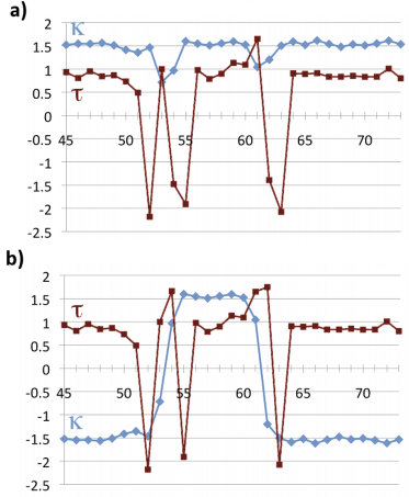
Figure 4: (Color online) The profile of $\kappa_{i}$ (light blue) and $\tau_{i}$ (dark red) along the 1YRF background. We use PDB indexing of the sites. In a) the $\kappa_{i}$ are restricted to $[0,\pi]$ and in b) this region is extended to $[-\pi,\pi]$ using (9).

Notice the irregular structure of the torsion angle $\tau_{i}$ in the loop (soliton) regions. A priori we expect from (14) that the torsion angle should have a regular profile. However, the numerical values that we compute from (14) are not restricted to the fundamental range $\tau_{i}\in[-\pi,\pi]$, they can take values beyond this range. The irregular structure of $\tau_{i}$ follows when we convert the values to the fundamental range, using $2\pi$ periodicity of $\tau_{i}$ in the discrete Frenet equation (8). Similarly we observe slight irregularity in the $\kappa_{i}$ profile. This can also be removed if we allow $\kappa_{i}$ to take values beyond $[-\pi,\pi]$ and use the $2\pi$ periodicity. But in the case of 1YRF the improvement in the precision turns out to be very small, and consequently we search for a solution of (19) by assuming that $\kappa_{i}\in[-\pi,\pi]$.

In Figure 5 we show the distribution of the side-chain angles ($\theta_{i},\varphi_{i}$) in YRF, by plotting the tips of the unit vector (21) on the two-sphere of Figure 2. As expected, they are located in the $\alpha$-helix region of Figure 2a) except along the loops, where they are located outside of the regular structure regions.

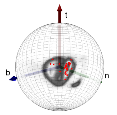
Figure 5: (Color online) The directional distribution of the side-chain angles ($\theta_{i},\varphi_{i}$). The background coincides with the annulus in Figure 2a).

We start by solving the classical equations of motion for $\kappa_{i}$ from (19). We then construct the remaining variables ($\tau_{i},\theta_{i},\varphi_{i}$) in terms of $\kappa_{i}$ using (14), (24) and (26); Since the ($\theta_{i},\varphi_{i}$) contributions to the $\kappa_{i}$ potential (16) are minuscule, we ignore the corresponding parameters in constructing the solution to the DNLS equation for $\kappa_{i}$. We use the iterative algorithm and procedure described in her , nora , and our results are summarized in Figure 6 and Table 1. We have been able to substantially improve the accuracy reported in nora , in particular for the first soliton. We now reach a RMSD accuracy less than 0.4 Ȧ even when we include the side-chain C_β atoms. The result is clearly within the Debye-Waller fluctuation distance regime that we compute from the experimental B-factors in the PDB data.

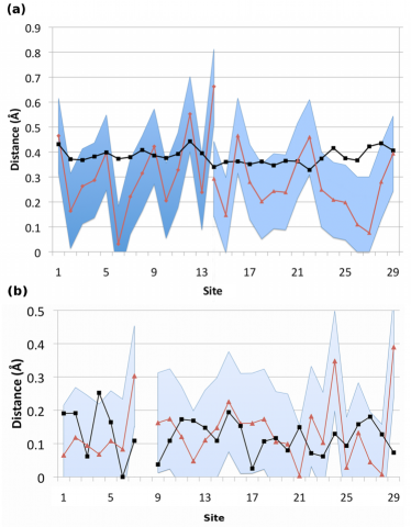
Figure 6: (Color online) Comparison between our soliton solutions in red (gray) and the experimental B-factor fluctuation distance of PDB data for 1YRF (black) along the backbone. In Figure a) for the C_α, and in Figure b) for the C_β where the experimental accuracy is estimated from (32). The shaded region describes the 0.15 Ȧ zero point fluctuations around solitons. The cut in Figure a) at sites 13-14 is where the two solitons overlap (Phe-58 in PDB), and the empty space in Figure b) is due to glycine that has no C_β.

parameter	soliton-1	soliton-2
$q_{1}$	0.459712	0.995867
$q_{2}$	4.5533320	9.408796
$m_{1}$	1.504535	1.550322
$m_{2}$	1.512836	1.535081
$a_{\tau}$	9.5752137e-9	7.840467e-6
$b_{\tau}$	-676965e-11	-4.973244e-9
$c_{\tau}$	4.875744e-9	4.2733696e-6
$d_{\tau}$	-2.917129e-9	-2.431388e-6
$a_{\theta}$	1.514770	1.322495
$b_{\theta}$	-0.0017952	-0.018619
$d_{\theta}$	0.0420877	6.930946e-8
$a_{\varphi}$	0.544859	0.3594184
$b_{\varphi}$	5.66111e-5	3.83253e-4
$d_{\varphi}$	-0.1845828	-0.226012
RMSD (Ȧ)	0.38	0.32

Table 1: Parameter values for the two-soliton solution that describes the two loops of 1YRF with a combined 0.39Ȧ accuracy for both C_α and C_β atoms. The displayed RMSD values are for the individual solitons. The soliton-1 is located at Glu-45 - Phe-58 and the soliton-2 is located at Phe-58 - Lys-73. We utilize scale invariance to set all $c_{\theta}=c_{\varphi}=1$. The result has sensitivity to the accuracy of parameters, because a folded protein is a piecewise linear polygonal chain with a positive Liapunov exponent.

In Figure 6a) we display the distance between the computed and the experimentally measured C_α atoms (excluding the N and C terminals). The shaded region in Figure 6a) describes the 0.15Ȧ zero point fluctuations peng around our solitons. For comparison, we also display the experimental Debye-Waller B-factor fluctuation distances, obtained from the PDB data. Except for the end point of soliton 1 (residue 58), our soliton solutions describe the backbone well within the limits of experimental accuracy.

In Figure 6b) we present our results for the C_β nutation, in comparison with the experimental data. We also present an estimate for the experimental uncertainties that we estimate as follows: The experimental B-factors give an estimate for the absolute fluctuation distance around the measured position. But now we are interested in estimating the (much smaller) relative error in the position of C_β with respect to the position of the ensuing C_α. For this we introduce the relative B-factor

$$B_{rel}\ =\ \left|B_{\alpha}-B_{\beta}\right|$$ (32)

In Figure 6b) we display the ensuing fluctuation distances that we have computed from the Debye-Waller relation using (32) in lieu of the B-factor. The precision of our computed results compare well with these experimental relative B-factor errors: For most of the sites the difference is no more than the 0.15Ȧ estimate for zero point fluctuations.

Finally, Figure 7 shows our soliton solution together with the 1YRF configuration in PDB.

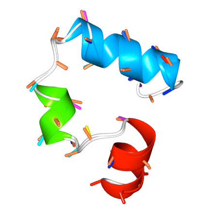
Figure 7: (Color online) A cartoon comparison of HP35 with our soliton solution summarized in Table 1. The combined C_α and C_β root-mean-square distance is 0.39 Ȧ which equals the experimental Debye-Waller B-factor fluctuation distance for the central carbons.

V Summary

In conclusion, the paradigm assumption that the tetrahedral covalent symmetry around the backbone C_α carbons is transferable, is correct to a good precision. However, with the advent of third and fourth generation X-ray sources there is now a rapid growth in the number of protein structures with sub-Ångström resolution. This makes it possible to scrutinize small corrections to this paradigm. We have found, that the backbone $N-C_{\alpha}-C$ bond angle shows systematic deviations from the ideal value, in a manner that is in direct correspondence with the corresponding secondary structure environment. We have investigated how this effect propagates to the orientation of the C_β carbon. We have found that the angular orientations of the C_β carbon similarly deviate from their ideal values, in a manner which is in a one-to-one correspondence with the underlying secondary structure environment.

We have presented a simple energy function that is based on the concept of universality, to model the secondary structure dependence in the C_β orientations. As an example, we have constructed the C_α-C_β backbone of HP35 villin, where we reach an accuracy that matches the experimental B-factor fluctuation distances. We propose that our observations and theoretical proposals could form a basis for the development of both more accurate refinement tools for experimental data analysis, and of more precise theoretical and computational MD force fields, to model the atomic level structure and dynamics of folded proteins.

References

- (1) I.W. Davis et.al., Nucl. Acids Res. 35 235 (2007)
- (2) R.A. Laskowski et.al., J. Biomol. NMR 8, 477 (1996)
- (3) X. Qu, R. Swanson, R. Day, J. Tsai, Curr. Protein Pept. Sci. 10, 270 (2009)
- (4) P.L. Freddolino, C.B. Harrison, Y. Liu, Y. Schulten, Nature Phys. 6, 751 (2010)
- (5) H.M. Berman et.al., Nucl. Acids Res. 28, W375 (2007)
- (6) L. Schäfer, M. Cao, Journ. Mol. Struc. 333, 201 (1995)
- (7) P.A. Karplus, Prot. Sci. 5, 1406 (1996)
- (8) D.S. Berkholz, M.V. Shapovalov, R.L. Dunbrack Jr., P. A. Karplus, Structure 17, 1316 (2009)
- (9) W.G. Touw, G. Vriend, Acta Cryst. D66, 1341 (2010)
- (10) P.G. Kevrekidis, The Discrete Nonlinear Schrödinger Equation: Mathematical Analysis, Numerical Computations and Physical Perspectives (Springer-Verlag, Berlin, 2009)
- (11) A.S. Davydov, Journ. Theor. Biol. 66, 379 (1977)
- (12) S. Hu, M. Lundgren, A.J. Niemi, Phys. Rev. E83, 061908 (2011)
- (13) M. Chernodub, S. Hu, A.J. Niemi, Phys. Rev. E82, 011916 (2010)
- (14) N. Molkenthin, S. Hu, A.J. Niemi, , Phys. Rev. Lett. 106, 078102 (2011)
- (15) S. Hu, A. Krokhotin, A.J. Niemi, X. Peng, Phys. Rev. E83, 041907 (2011)
- (16) B. Widom, J. Chem. Phys. 43, 3892 (1965).
- (17) L.P. Kadanoff, Physics 2, 263 (1966).
- (18) K.G. Wilson, Phys. Rev. B4, 3174 (1971).
- (19) M.E. Fisher, Rev. Mod. Phys. 46, 597 (1974).
- (20) A.J. Niemi, Phys. Rev. D67, 106004 (2003)
- (21) U.H. Danielsson, M. Lundgren, A.J. Niemi, Phys. Rev. E82, 021910 (2010)
- (22) A. Krokhotin, A.J. Niemi, X.Peng, Phys. Rev. E85, 031906 (2012)
- (23) J. Meng, D. Vardar, Y. Wang, H.C. Guo, J.F. Head, C.J. McKnight, Biochemistry 44, 11963 (2005)
- (24) T.K. Chiu, J. Kubelka, R. Herbst-Irmer, W.A. Eaton, J. Hofrichter, D.R. Davies, Proc. Natl. Acad. Sci. U.S.A 102, 7517 (2005)
- (25) L. Wickstrom, Y. Bi, V. Hornak, D.P Raleigh, C. Simmerling, Biochemistry 46, 3624 (2007)
- (26) D.L. Ensign, P.M. Kasson, V.S. Pande, J. Mol. Biol. 374, 806 (2007)
- (27) H. Lei, Y. Duan, J. Mol. Biol. 370, 196 (2007)
- (28) P.L. Freddolino, K. Schulten, Biophys. Journ. 97, 2338 (2009)
- (29) D.E. Shaw et.al., Science 330, 341 (2010)
- (30) M. Herrmann, Applic. Anal. 89, 1591 (2010)