Longitudinal magnetic excitation in KCuCl₃ studied by Raman scattering under hydrostatic pressures

Abstract

We measure Raman scattering in an interacting spin-dimer system KCuCl₃ under hydrostatic pressures up to 5 GPa mediated by He gas. In the pressure-induced quantum phase, we observe a one-magnon Raman peak, which originates from the longitudinal magnetic excitation and is observable through the second-order exchange interaction Raman process. We report the pressure dependence of the frequency, halfwidth and Raman intensity of this mode.

1 Introduction

The magnetic-field and pressure-induced quantum phase transitions in TlCuCl₃ and KCuCl₃ have been extensively studied.[1, 2] In the spin-gapped phase, the $S=1/2$ interacting antiferromagnetic (AF) spin dimer system has a spin-triplet excited state separated from the spin-singlet ground state. Because of the magnetic interaction between spin dimers, the excited state is dispersive and then the spin-gap energy is much lower than that of the isolated spin dimers. This is described by the bond-operator model.[3] The Zeeman effect under a magnetic field, the increase of interdimer interaction under high pressure and/or the impurity doping cause the quantum phase transition to the ordered phase. The ordered phase is characterized by the absence of the spin gap and the AF ordered moment of which amplitude can fluctuate. This fluctuation is the longitudinal magnetic excitation which we focus on in this paper.

As well as inelastic neutron scattering (INS), the inelastic light scattering, known as Raman scattering, is a powerful tool to detect the longitudinal magnetic excitation.[4] In the quantum phase induced by magnetic field, the longitudinal magnon excitation is detected as a one-magnon Raman peak induced through the second-order exchange interaction Raman process.[5, 6] Comparing INS, only a small size of sample is enough to measure Raman scattering. Using the diamond anvil cell (DAC), we can apply hydrostatic pressure up to about 10 GPa. These are advantages of Raman scattering. In this paper, we report the one-magnon Raman scattering in the pressure-induced ordered phase of KCuCl₃.

2 Experiments

The single crystal of KCuCl₃ was grown from a melt by the standard Bridgeman technique. A small piece of it with a size of 100 $\times$ 50 $\times$ 10 $\mu$m was enclosed into DAC. And then, the DAC was placed in a continuous flow type cryostat to cool the single crystal down to 3 K.

We used He gas as a pressure medium because it gives almost hydrostatic conditions.[7, 8]Moreover, the single crystal is easily dissolved in methanol-ethanol mixture, which is a standard pressure medium. The pressure $P$ was monitored by using the wavelength shift of the $R_{1}$ fluorescence line of a ruby powder. Because the wavelength of the $R_{1}$ fluorescence line depends on temperature, we set ruby powder in high pressure section and in the ambient pressure one (on the back surface of diamond). Because we can detect the $R_{1}$ fluorescence peaks from the ruby powder at the high pressure section and that at the ambient pressure one simultaneously, this method estimates very precise pressure at low temperatures.

Raman scattering was excited by an Ar⁺-ion laser with the wavelength of 514.5 nm. The scattered light was dispersed by using a triple grating monochromator (Jobin-Yvon T64000) and was detected by a CCD detector cooled by liquid-N₂. In order to observe the magnon Raman spectra strongly, the incident laser was polarized along the direction of the strong interdimer interaction, which is almost parallel to the one along the intradimer interaction,[5] and we did not use the analyzer (polarizer) in front of the entrance slit of the monochromator. The Raman shift was calibrated by using a rotational Raman spectrum of air.

3 Results

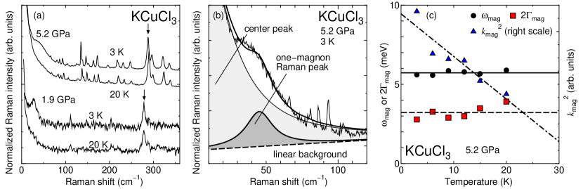
Figure 1: (a) Raman spectra at 3 and 20 K under pressures of 1.9 and 5.2 GPa. (b) Low-energy Raman spectrum at 3 K under 5.2 GPa and its decomposition. (c) Temperature dependences of the frequency $\omega_{\rm mag}$, halfwidth $2\Gamma_{\rm mag}$ and squared coupling coefficient $k^{2}_{\rm mag}$ of the one-magnon Raman peak at 1.9 GPa. The details of the fitting are written in text.

Figure 1(a) shows Raman spectra at 3 and 20 K under pressures of 1.9 and 5.2 GPa. The Raman intensity was normalized by the integrated intensity of the Raman peak around 300 cm^-1 in each spectrum, which is indicated by an arrow in Fig. 1(a). The overall phonon Raman spectrum above 50 cm^-1 is consistent with the one in the previous report at ambient pressure.[9] The frequencies of the phonon peaks increase with increasing pressure. Using this fact, we can obtain the mode Grüneisen constant. However, it is beyond of the scope of this paper and will be presented elsewhere. One can see that the Raman peak around 25 cm^-1 at 3 K under $P$ = 1.9 GPa is superimposed on the strong tail centered at 0 cm^-1 which comes from the stray light of the reflection and the Rayleigh scattering. This peak was not observed at 20 K. As will be discussed in the following, this is the one-magnon Raman peak from the longitudinal magnon excitation.

Figure 1(b) describes the fitting procedure at $P$ = 5.2 GPa. For quantitative discussion, we extract the one-magnon Raman peak $I_{\rm mag}(\omega)$ from the observed Raman spectrum $I_{\rm obs}(\omega)$, by using the nonlinear least square fit with the model of two Lorentz functions on a linear background:

$$I_{\rm obs}(\omega)\equiv I_{\rm mag}(\omega)+\frac{k_{\rm c}^{2}\Gamma_{\rm c}}{\omega^{2}+\Gamma_{\rm c}^{2}}+(a\omega+b)=\frac{[n(\omega_{\rm mag})+1]k_{\rm mag}^{2}\Gamma_{\rm mag}}{(\omega-\omega_{\rm mag})^{2}+\Gamma_{\rm mag}^{2}}+\frac{k_{\rm c}^{2}\Gamma_{\rm c}}{\omega^{2}+\Gamma_{\rm c}^{2}}+(a\omega+b)\ ,$$ (1)

where $\omega_{\rm mag}$, $k_{\rm mag}$ ($k_{\rm c}$), $\Gamma_{\rm mag}$ ($\Gamma_{\rm c}$), $n(\omega_{\rm mag})$ and $(a\omega+b)$ denote the frequency, the coupling coefficient and the halfwidth of the one-magnon mode (the strong tail at 0 cm^-1), the Bose factor and the linear background, respectively,

Figure 1(c) shows the temperature dependences of $\omega_{\rm mag}$, $2\Gamma_{\rm mag}$ and the squared coupling coefficient $k_{\rm mag}^{2}$. One can see that $k_{\rm mag}^{2}$ decreases with increasing temperature, while $\omega_{\rm mag}$ and $2\Gamma_{\rm mag}$ are almost independent of temperature. And therefore, we estimate $k_{\rm mag}^{2}$, $\omega_{\rm mag}$ and $2\Gamma_{\rm mag}$ at zero temperature. With the values obtained under different pressures, we show the pressure dependences of $\omega_{\rm mag}$, $2\Gamma_{\rm mag}$ and $k_{\rm mag}^{2}$ as functions of applied pressure in Fig. 2.

4 Discussion

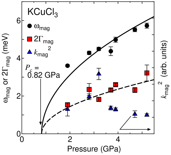
Figure 2: Pressure dependences of the frequency $\omega_{\rm mag}$, halfwidth $2\Gamma_{\rm mag}$ and squared coupling coefficient $k^{2}_{\rm mag}$ of the one-magnon Raman peak.

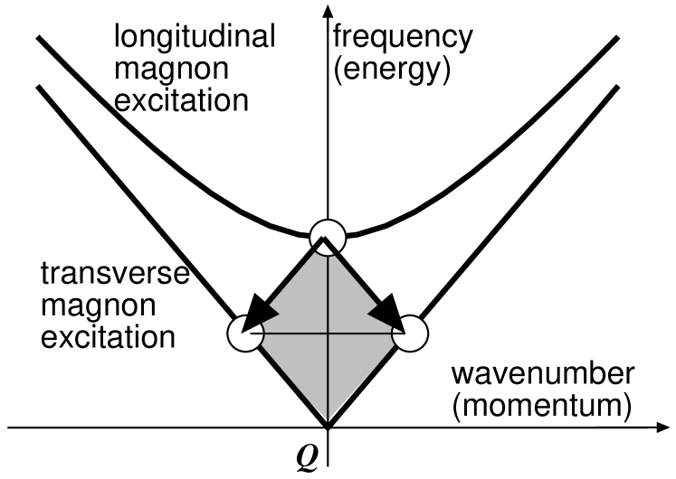
Figure 3: Schematic of a decay process from one longitudinal magnon to two transverse magnons in the energy-momentum space. ${\bm{Q}}$ denotes the magnetic zone center.

We observed that the frequency and halfwidth of the one-magnon Raman peak are proportional to a function of $(1-P/P_{\rm c}^{\rm K})^{1/2}$, where the critical pressure $P_{\rm c}^{\rm K}$ (= 0.82 GPa) was obtained by magnetization measurement under hydrostatic pressures.[10] First, we compare these results to the results of INS in TlCuCl₃ taken under hydrostatic pressures.[11] The frequency and halfwidth of the longitudinal magnetic excitation are proportional to a function of $(1-P/P_{\rm c}^{\rm Tl})^{1/2}$ in TlCuCl₃, where $P_{\rm c}^{\rm Tl}$ $\sim$ 0.1 GPa. Then we conclude that the one-magnon Raman peak observed at low temperatures under higher pressures than 0.82 GPa comes from the longitudinal magnetic excitation through the second-order exchange interaction magnon Raman process.[4]

We focus on the halfwidth $\Gamma_{\rm mag}$ proportional to the frequency $\omega_{\rm mag}$. Because $2\Gamma_{\rm mag}$ corresponds to the inverse lifetime of magnon, we consider the decay process of the longitudinal magnetic excitation. In the bond-operator model, the terms of two spin scalar product in the spin Hamiltonian and the effective magnon Raman operator are expressed as the quadratic terms of the singlet and triplet operators.[4, 5, 6] In the ordered phase, these operators are mixed with each other and the system can be rewritten by using the quadratic terms of the four mixed singlet-triplet operators. Because one of these four can be treated as the uniformly condensed mean-field operator ($c$-number operator, $\overline{a}$ in ref. [3]), the interdimer interaction can be written by using three kinds of operators ($b_{{\bm{k}}{\rm L}}$, $b_{{\bm{k}}y}$ and $b_{{\bm{k}}z}$ in ref. [3], where $\hbar{\bm{k}}$ is the momentum of magnon). Here $b_{{\bm{k}}{\rm L}}$ is the annihilation operator of the longitudinal magnetic excitation and the other two are those of the transverse ones.[3, 4] The spin Hamiltonian and the effective Raman operator contain the terms of ${\cal O}(b)$, ${\cal O}(b^{2})$, ${\cal O}(b^{3})$ and ${\cal O}(b^{4})$, where $b$ denotes one of $b_{{\bm{k}}{\rm L}}$, $b_{{\bm{k}}{\rm L}}^{\dagger}$, $b_{{\bm{k}}y}$, $b_{{\bm{k}}y}^{\dagger}$, $b_{{\bm{k}}z}$ and $b_{{\bm{k}}z}^{\dagger}$. To minimize the magnetic energy, the ${\cal O}(b)$ term in the spin Hamiltonian should vanish. We note here that the ${\cal O}(b)$ term in the Raman operator can be finite even in this case. This is the origin of the one-magnon Raman scattering.[4, 5] The magnon dispersion curve comes from the ${\cal O}(b^{2})$ terms in the exchange interaction.[3] From an analogy with the anharmonicity problem of phonons, one can easily show that the ${\cal O}(b^{3})$ term gives the finite lifetime of magnon due to the magnon-magnon decay in Fig. 3, which is omitted in refs. [3] and [4].

We consider the magnon-magnon decay channel discussed by Kulik and Sushkov [12] for the lifetime of the longitudinal magnetic excitation at the magnetic $\Gamma$ point ${\bm{Q}}$. This Raman-active mode is massive and its dispersion curve around ${\bm{Q}}$ is proportional to $|{\bm{Q}}|^{2}$ with the minimum energy at ${\bm{Q}}$. Below this energy, there exists only two branches of the magnetic excitations, i.e., two transverse modes. These are the Goldstone modes of which dispersion curve around ${\bm{Q}}$ have a linear function of $|{\bm{Q}}|$. The possible magnon-magnon decay channel can be found easily by using the geometric procedure on the energy-momentum space, as shown in Fig. 3. Because the number of decay channels is proportional to $\omega_{\rm mag}^{2}$, the transition probability for one channel should be proportional to $\omega_{\rm mag}^{-1}$, resulting in the halfwidth proportional to $\omega_{\rm mag}$. These can be calculated by using the bond-operator method, which will be published elsewhere.

The bond operator theory predicts that $k_{\rm mag}^{2}\propto(1-P/P_{\rm c}^{\rm K})^{1/2}$,[4] which is inconsistent with our observation. The strong tail at 0 cm^-1 might be a possible origin of this deviation. As we stated, we normalized the squared coupling coefficient by that of the phonon mode around 300 cm^-1, i.e., we implicitly suppose the pressure independent properties of this phonon. We omit the Raman intensity through the three magnon Raman process, which was observed at ambient pressure.[9] These are other possible origins of this deviation.

References

References

- [1] Tanaka H, Takatsu K, Shiramura W and Ono T 1996 J. Phys. Soc. Jpn. 65 1945
- [2] Takatsu K, Shiramura W and Tanaka H 1997 J. Phys. Soc. Jpn. 66 1611.
- [3] Matsumoto M, Normand B, Rice T M and Sigrist M 2004 Phys. Rev. B 69 054423
- [4] Matsumoto M, Kuroe H, Oosawa A and Sekine T 2008 J. Phys. Soc. Jpn. 77 033702
- [5] Kuroe H, Kusakabe K, Oosawa A, Sekine T, Yamada F, Tanaka H and Matsumoto M 2008 Phys. Rev. B 77 134420
- [6] Kuroe H, Kusakabe K, Oosawa A, Sekine T, Yamada F, Tanaka H and Matsumoto M 2008 Proc. 21st Int. Conf. on Raman Spectroscopy (ICORS 2008) p 631
- [7] Takemura K and Dewaele A 2008 Phys. Rev. B 78 104119
- [8] More precisely, we need to use the term of quasi-hydrostatic pressure. However, because of the strong zero-point oscillation, high pressure He gas serves very high hydrostaticity even when it is frozen at low temperature.
- [9] Choi K -Y, Oosawa A, Tanaka H, and Lemmens P 2005 Phys. Rev. B 72 024451
- [10] Goto K, Fujisawa M, Tanaka H, Uwatoko Y, Oosawa A, Osakabe T and Kakurai K 2006 J. Phys. Soc. Jpn. 75 064703
- [11] Rüegg Ch, Normand B, Matsumoto M, Furrer A, McMorrow D F, Krämer K W, Güdel H -U Gvasailiya S N, Mutka H and Boehm M 2008 Phys. Rev. Lett. 100 205701
- [12] Kulik Y and Sushkov O P 2011 Preprint arXiv:1104.1245