The June 2012 transit of Venus.
Framework for interpretation of observations

Abstract

Context. Ground-based observers have on 5–6th June 2012 the last opportunity of the century to watch the passage of Venus across the solar disk from Earth. Venus transits have traditionally provided unique insight into the Venus atmosphere through the refraction halo that appears at the planet’s outer terminator near ingress/egress. Much more recently, Venus transits have attracted renewed interest because the technique of transits is being succesfully applied to the characterization of extrasolar planet atmospheres.

Aims. The current work investigates theoretically the interaction of sunlight and the Venus atmosphere through the full range of transit phases, as observed from Earth and from a remote distance. Our model predictions quantify the relevant atmospheric phenomena, thereby assisting the observers of the event in the intepretation of measurements and the extrapolation to the exoplanet case.

Methods. Our approach relies on the numerical integration of the radiative transfer equation, and includes refraction, multiple scattering, atmospheric extinction and solar limb darkening, as well as an up-to-date description of the Venus atmosphere.

Results. We produce synthetic images of the planet’s terminator during ingress/egress that demonstrate the evolving shape, brightness and chromaticity of the halo. Our simulations reveal the impact of micrometer-sized aerosols borne in the upper haze layer of the atmosphere on the halo’s appearance. Guidelines are offered for the investigation of the planet’s upper haze from vertically-unresolved photometric measurements. In this respect, the comparison with measurements from the 2004 transit appears encouraging. We also show integrated lightcurves of the Venus-Sun system at various phases during transit and calculate the respective Venus-Sun integrated transmission spectra. The comparison of the model predictions to those for a Venus-like planet free of haze and clouds (and therefore a closer terrestrial analogue) complements the discussion and sets the conclusions into a broader perspective.

1 Introduction

This year, from about 22:10UT June 5 to 04:50UT June 6, observers across the Earth’s illuminated hemisphere have the opportunity to watch Venus passing in front of the solar disk. The transits of Venus visible from Earth are regularly spaced in intervals of 8, 105.5, 8 and 121.5 years. After the June 2004 transit, this year’s event is the last one before 2117.

Venus transits occupy a notable place in the history of astronomy and planetary sciences. Following Halley’s suggestion that Venus transits might provide a measure of the terrestrial parallax, the events of the 18th and 19th centuries helped estimate the Earth-Sun distance. Also, it is often quoted that the 1761 transit provided the first evidence for the Venus atmosphere (Link, link1959 (1959)). Lomonosov correctly attributed the halo that appears at the planet’s outer terminator during ingress/egress to sunlight rays refracted towards the Earth on their passage through the Venus atmosphere. The subsequent transits of 1769, 1874 and 1882 provided additional opportunities for the investigation of the phenomenon and, in turn, of the Venus atmosphere. Since then, a number of theories have been issued to interpret the halo and its connection with the Venus atmospheric structure. A discussion of them and of other phenomena related to refraction in planetary atmospheres is presented by Link (link1969 (1969)).

An additional reason for pursuing planetary transits has emerged recently. The discovery of planets in orbit around stars other than our Sun has opened up a new and rapidly-growing field in astrophysics (Mayor & Queloz, mayorqueloz1995 (1995)). Some of those planets happen to periodically intercept the Earth-to-star line of sight, thereby causing a dimming in the apparent stellar brightness. In combination with some form of spectral discrimination, the so-called technique of transits may provide valuable insight into the composition and state of the planets’ atmospheres (e.g. Seager & Deming, seagerdeming2010 (2010), and refs. therein). In our Solar System, only Mercury and Venus are observable from Earth while transiting the Sun. Since Mercury’s atmosphere is tenuous, the Venus transits of 2004 and 2012 represent unique occasions for testing the technique of transits on an Earth-sized planet hosting a dense atmosphere, a major goal in the near-future exploration of extrasolar planets.

The interest raised by the 2004 and 2012 Venus transits is apparent (Ambastha et al., ambasthaetal2006 (2006); Ehrenreich et al., ehrenreichetal2012 (2012); Hedelt et al., hedeltetal2011 (2011); Kopp et al., koppetal2005 (2005); Pasachoff et al., pasachoffetal2011 (2011); Schneider et al., schneideretal2004 (2004, 2006); Tanga et al., tangaetal2012 (2012)). An ambitious international plan of observations from both Earth-based and space-borne observatories is underway for the 2012 event (Pasachoff, pasachoff2012 (2012)). It thus seems appropriate to review the theory of planetary transits in its specific application to the Venus transit, taking advantage of recent progress in the characterization of the Venus atmosphere and of modern computational capacity.

This work addresses the interaction of sunlight and the Venus atmosphere during transit. Descriptions of the formulation and the prescribed model parameters are given in §2. Section §3 investigates the shape, brightness and chromaticity of the halo. Section §4 establishes the connection between the halo and the in-transit signature of the Venus atmosphere, and presents the lightcurves of the Venus-Sun system as observed from Earth and remotely. Section §5 summarizes the main predictions. Ultimately, it is hoped that our model predictions can serve as guidelines in the interpretation of the observations to come.

2 Refractive theory of the Venus transit

Lunar eclipses and planetary transits are conceptually similar phenomena that admit a common formal treatment (Link, link1969 (1969)). García Muñoz & Pallé (garciamunozpalle2011 (2011)) revisited the theory of lunar eclipses. Their formulation was subsequently used in the interpretation of a partial lunar eclipse (García Muñoz et al., garciamunozetal2011 (2011)), and to investigate the impact of refraction on the in-transit signature of Earth-like extrasolar planets (García Muñoz et al., garciamunozetal2012 (2012)). We now apply the formulation to the Venus transit. Since the refractive theory of planetary transits has thus far received marginal attention, we expend some effort describing the model approach.

2.1 The Radiative Transfer Equation (RTE)

The steady-state RTE for a refractive medium in the geometrical optics limit has been presented by, e.g., Zheleznyakov (zheleznyakov1967 (1967)) and Énomé (enome1969 (1969)):

$$\mathbf{s}\cdot\nabla\left(\frac{L\mathbf{(x,s)}}{n^{2}\mathbf{(x)}}\right)=-\gamma(\mathbf{x})\frac{L\mathbf{(x,s)}}{n^{2}\mathbf{(x)}}+\frac{J\mathbf{(x,s)}}{n^{2}\mathbf{(x)}}.$$ (1)

Here, $L\mathbf{(x,s)}$ is the radiance at $\mathbf{x}$ in direction ${\bf{s}}$, $\gamma(\mathbf{x})$ and $n(\mathbf{x})$ stand for the extinction coefficient and index of refraction of the medium, respectively, and $J\mathbf{(x,s)}$ is the source term, which may include separate terms for scattered radiation and emission from within the medium. $L\mathbf{(x,s)}$, $\gamma(\mathbf{x})$, $n(\mathbf{x})$ and other associated magnitudes are wavelength dependent, which should be explicitly stated in the notation. For simplicity, however, that characteristic is omitted throughout the text. The boundary conditions for the direct and diffuse components of Eq. (1) are introduced in §2.2 and 2.3, respectively.

For $n(\mathbf{x})$ constant, Eq. (1) turns into the well-known RTE for a non-refractive medium. In that case, the photons follow straightline trajectories between scattering events. For a non-absorbing, non-emitting, non-scattering medium ($\gamma(\mathbf{x})$$\equiv$$J(\mathbf{x})$$\equiv$0) with possibly spatially-dependent $n(\mathbf{x})$, Eq. (1) reduces to the conservation of ${L\mathbf{(x,s)}}/{n^{2}\mathbf{(x)}}$ on the refraction-bent ray trajectories. That magnitude is sometimes referred to as the Clausius invariant, and generalizes the conservation of radiance in media of constant index of refraction.

As in radiometry of non-refractive media, the irradiance, or net flux of light that crosses an elementary surface of normal vector ${\bf{n_{x_{O}}}}$ (not to be mistaken for the index of refraction at $\mathbf{x_{O}}$, $n(\mathbf{x_{O}})$) from directions $\mathbf{s_{O}}$, at the observer’s location $\mathbf{x_{O}}$ is obtained by integrating the directional radiance ${{L}}({\bf{x_{O}}},{\bf{s_{O}}})$ over solid angle:

$$F({\bf{x_{O}}})=\int_{\partial\Omega=\partial\Omega_{\venus}\cup\partial\Omega_{\odot}}{{{L}}({\bf{x_{O}}},{\bf{s_{O}}}){{\bf{s_{O}}}\cdot{\bf{n_{x_{O}}}}}d{\Omega(\bf{s_{O}})}.}$$ (2)

In the general application of Eq. (2) to the Venus transit, the integration domain must contain the solid angles subtended from $\mathbf{x_{O}}$ by planet and atmosphere together, $\partial\Omega_{\venus}$, and the Sun, $\partial\Omega_{\odot}$.

For the numerical evaluation of Eq. (2), it is convenient to work with auxiliary variables. Concentrating for now on the integral over $\partial\Omega_{\venus}$, introducing:

$$\mu={\bf{s_{O}}}\cdot{\bf{n_{x_{O}}}},$$

and the azimuthal angle $\phi$, using:

$$d{\Omega(\bf{s_{O}})}=d\mu d\phi,$$

and the normalized variables:

$$\xi=(\mu^{2}-\mu^{2}_{\rm{M}})/(\mu^{2}_{\rm{m}}-\mu^{2}_{\rm{M}})\;\;\rm{and}\;\;\eta={\phi}/{\pi},$$

Eq. (2) can be rewritten as:

$$F({\bf{x_{O}}})=\pi(\mu^{2}_{m}-\mu_{M}^{2})\int_{0}^{1}\int_{0}^{1}L(\xi,\eta)d\xi d\eta,$$ (3)

where:

$$\mu^{2}_{\rm{M}}=1-(r_{\rm{TOA}}/d_{\rm{\bf{O}}})^{2},$$

$$\mu^{2}_{\rm{m}}=1-(R_{\venus}/d_{\rm{\bf{O}}})^{2},$$

$$r_{\rm{TOA}}=R_{\venus}+h_{\rm{TOA}},$$

$R_{\venus}$ is the Venus mean radius, $h_{\rm{TOA}}$ is the top of the atmosphere altitude, and $d_{\rm{\bf{O}}}$ is the observer-to-Venus centre distance. We may also define the impact radius $r_{b}$ for each $\mu^{2}$ through:

$$\mu^{2}=1-(r_{b}/d_{\rm{\bf{O}}})^{2}.$$

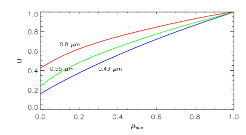
Figure 1: Limb darkening function $U$($\mu_{\odot}$) at selected wavelengths. For a color version of the figure, see the electronic journal.

Here, $r_{b}$ has the meaning of the distance of closest approach to the Venus centre for straightline rays traced sunwards from $\mathbf{x_{O}}$. Essentially, Eq. (3) maps the original integral onto a plane of incident directions $\mathbf{s_{O}}$={$\xi,\eta$} sampling the field of view from $\mathbf{x_{O}}$. Figure 1 in García Muñoz & Pallé (garciamunozpalle2011 (2011)) sketches the meaning of some of the variables introduced above.

2.2 The direct component of sunlight

The usual treatment of the RTE separates the direct and diffuse components. Neglecting the emission from within the medium and taking ${J\mathbf{(x,s)}}$$\equiv$0, one obtains for the direct radiance:

$$\frac{L_{D}\mathbf{(x_{O},s_{O})}}{n^{2}\mathbf{(x_{O})}}=\frac{L_{D}\mathbf{(x_{\odot},s_{\odot})}}{n^{2}\mathbf{(x_{\odot})}}\exp{[-\int_{\Gamma}\gamma{(s)}ds]},$$ (4)

for ray trajectories $\Gamma$ connecting $\mathbf{x_{O}}$ and the solar disk. Here, $s$ is the path length on the ray trajectory and ${\bf{x_{\odot}}}$ and ${\bf{s_{\odot}}}$ are the location and direction of departure of the sunlight ray on the solar disk. The squared refraction indices at the observer’s site and at the Sun’s photosphere, ${n^{2}\mathbf{(x_{O})}}$ and ${n^{2}\mathbf{(x_{\odot})}}$ respectively, can be taken as $\approx$1 in Eq. (4) at visible and near-infrared wavelengths. $L_{D}\mathbf{(x_{\odot},s_{\odot})}$ is the radiance emitted by the Sun and enters the formulation as a boundary condition. We assume that it depends on the emission angle, $\cos^{-1}(\mu_{\odot})$, through a polynomial of the form $U$= $\sum_{i=0}^{5}u_{i}\mu^{i}_{\odot}$, and that the wavelength-dependent coefficients $u_{i}$ account for the chromatic effects in the solar output. A good representation of the solar output near the Sun’s edge, $\mu_{\odot}$$\rightarrow$0, is important for the simulation of the ingress/egress phases of the transit. The adopted wavelength-dependent limb-darkening coefficients $u_{i}$ are from Pierce & Slaughter (pierceslaughter1977 (1977)) and Pierce et al. (pierceetal1977 (1977)). Generally, the coefficients are dependent on the star’s metallicity, a fact that must properly be accounted for in the analysis of extrasolar planet lightcurves (Claret, claret2000 (2000); Sing, sing2010 (2010)). Thus, $L_{D}\mathbf{(x_{\odot},s_{\odot})}$=$B_{\odot}U$, where $B_{\odot}$ is the stellar radiance at the Sun’s center, $\mu_{\odot}$=$1$. (Note also that $\sum_{i=0}^{5}u_{i}$=1.) Figure (1) shows the implemented $U$($\mu_{\odot}$) at selected wavelengths.

Considering the above, to a good approximation:

$$L_{D}\mathbf{(x_{O},s_{O})}=B_{\odot}U\exp{[-\int_{\Gamma}\gamma{(s)}ds]},$$ (5)

which is the Beer-Lambert law of extinction in a non-refractive medium. Using Eq. (5) does not mean that refraction plays a minor role in the formulation. Refraction enters $L_{D}\mathbf{(x_{O},s_{O})}$ at the time of devising the ray trajectory $\Gamma$. For that purpose, we use the tracing scheme based on path length by van der Werf (vanderwerf2008 (2008)) and trace each ray trajectory from ${\bf{x_{O}}}$ sunwards after specifying the Venus atmospheric profile for the wavelength-dependent refraction index.

For the evaluation of Eq. (3) over $\partial\Omega_{\venus}$, the $\xi$–$\eta$ field of view at $\mathbf{x_{O}}$ is subdivided into $N_{\xi}$$\times$$N_{\eta}$ (=200$\times$360) evenly-sized bins, each of them associated with an incident direction $\mathbf{s_{O}}$. For each direction $\mathbf{s_{O}}$={$\xi,\eta$} a ray trajectory $\Gamma$ is traced, and the corresponding optical opacity going into Eq. (5) is calculated. The rays failing to connect $\mathbf{x_{O}}$ with the solar disk have $L_{D}\mathbf{(x_{O},s_{O})}$$\equiv$0. In the halo, during ingress/egress, $L_{D}\mathbf{(x_{O},s_{O})}$$\equiv$0 occurs for rays crossing nearly unrefracted through the upper layers of the atmosphere, but also for rays passing through the lowermost altitudes and whose trajectories become deflected away from the Sun. During transit, the trajectories failing to connect $\mathbf{x_{O}}$ with the solar disk impose a ring of altitudes at the planet’s terminator that cannot be probed from a remote distance. The latter is discussed in detail by García Muñoz et al. (garciamunozetal2012 (2012)) and will be noted again for the specific case of Venus in §3.1 and 4.1. By going through the entire $N_{\xi}$$\times$$N_{\eta}$ matrix of directions ${\bf{s_{O}}}$, the image of the solar disk at ${\bf{x_{O}}}$ emerging from the planet’s terminator is constructed.

We could adopt the same strategy to evaluate Eq. (3) over the rest of $\partial\Omega$ not contained in $\partial\Omega_{\venus}$. This is, however, rather inefficient given the large ratio of Sun/Venus radii, $R_{\odot}/R_{\venus}$. Instead, we integrate analytically the irradiance over the unobstructed view of the star, $F_{\odot}$=$\pi$$(R_{\odot}/l_{\odot})^{2}$$\sum_{i=0}^{5}2u_{i}/(i+2)$, where $l_{\odot}$ is the observer-to-Sun centre distance, and subtract the part corresponding to $\partial\Omega_{\venus}$ calculated by Monte Carlo integration.

Taking the observer’s location $\mathbf{x_{O}}$ for carrying out the integration of Eq. (3) for the direct sunlight component is in line with the early formulations of the photometric theory of lunar eclipses (Link, link1962 (1962), link1969 (1969)). Link (link1969 (1969)), in Section 1.2.21 of that monograph, comments on the equivalence of that approach with other formulations that alternatively carry out the integration at the solar plane. Link (link1969 (1969)) also refers to the so-called attenuation by refraction that occurs by the compression of the solar disk image at the planet’s terminator during ingress/egress, and notes that its effect is implicitly accounted for in the projection of $d\Omega(\mathbf{s_{O}})$ on the solar disk. Attenuation by refraction occurs always that sunlight rays traverse a planet’s stratified atmosphere (Hays & Roble, haysroble1968 (1968)), and merely represents the change in cross section undergone by a pencil of sunlight rays upon crossing the stratified medium.

Figure (2) offers some visual insight into this point. The rays in the sketch are evenly spaced in angle at their departure from $\mathbf{x_{O}}$ towards the Sun. The rays gradually separate as they traverse the atmosphere due to differential refraction between altitude layers. Assuming that the atmosphere is transparent and solar limb darkening is omitted, Eq. (3) would simply lead to a measure of the halo’s angular size perceived at $\mathbf{x_{O}}$. Since in such conditions the radiance is very approximately conserved on ray trajectories, the contribution of a solar disk surface element is ultimately limited by the size of its refracted image at the planet’s terminator. Sidis & Sari (sidissari2010 (2010)) set out from this conclusion to evaluate the halo’s overall brightness for transiting extrasolar giant planets with transparent atmospheres. The factor by which the pencil’s cross section is compressed depends on both the Sun-Venus and Venus-observer distances as well as on the atmosphere’s refractive properties. Figure (3) sketches the integration of the direct radiance over a differential element of solid angle at the observer’s site.

2.3 The diffuse component of sunlight

A fraction of the sunlight photons incident on Venus is redirected in the forward direction after one or more scattering collisions with the medium. To estimate the contribution of diffuse sunlight, we must solve the RTE including:

$$J\mathbf{(x,s)}=\beta(\mathbf{x})\int_{\partial\Omega_{\venus}}p\mathbf{(x,s,s^{\prime})}L\mathbf{(x,s^{\prime})}d\Omega(\mathbf{s^{\prime}})$$ (6)

as a source term of the equation, with $\beta(\textbf{x})$ being the medium’s scattering coefficient and $p\mathbf{(x,s,s^{\prime})}$ the normalized phase function for changes $\mathbf{s^{\prime}}$$\rightarrow$$\mathbf{s}$ in the direction of light propagation. The given $J\mathbf{(x,s)}$ is identical to the form of the scattering term in non-refractive media (Ben-Abdallah et al., benabdallahetal2001 (2001); Kowalski & Saumon, kowalskisaumon2004 (2004); Fumeron et al., fumeronetal2005 (2005)). The integration over the part of $\partial\Omega$ not included in $\partial\Omega_{\venus}$ is unnecessary if the top of the atmosphere is placed high enough.

Working in a refractive medium presents two additional subtleties in the treatment of the diffuse RTE. First, the radiance is affected by the reciprocal of $n^{2}(\mathbf{x})$, although we are allowed to take $n(\mathbf{x})$$\approx$1 at the relevant wavelengths. Second, the photon trajectories in between scattering events follow refraction-bent trajectories. However, scattering itself alters the direction of light propagation by angles likely to exceed the deflection caused by refraction. We may therefore also omit this aspect, and treat the diffuse RTE as in a non-refractive medium.

The practical solution to Eqs. (1) and (6) is carried out by Monte Carlo integration (O’Brien, obrien1992 (1992); García Muñoz & Pallé, garciamunozpalle2011 (2011)) with the proper expression for $F_{\odot}$ at the Venus orbital distance as a boundary condition. The scheme is nested in the simultaneous integration of Eq. (3) over the Venus disk.

2.4 The reference Venus atmosphere

Traditionally, observations of Venus during ingress/egress have provided valuable information on the tilt of the planet’s rotational axis and equator-to-pole variations in the atmospheric structure (Link, link1959 (1959)). Thus, for the simulations we require a description of the atmospheric optical properties on a global scale as well as the latitudinal dependence for some of them.

For the temperature, we adopted the Seiff et al. (seiffetal1985 (1985)) profile for a latitude of 45^∘ up to 100 km and the Hedin et al. (hedinetal1983 (1983)) noon profile there upwards. The atmosphere was assumed to be composed of CO₂–N₂ in a 96.5–3.5% proportion, and the background density was obtained by integrating the hydrostatic balance equation.

At the altitudes at which the atmosphere becomes optically thick, the opacity is largely dictated by aerosols rather than by the atmospheric gas. Thus, latitudinal variations in the gas profile are expected to be of less importance than the respective variations in the aerosol loading. Similarly, the errors introduced in the refracted angles from neglecting the latitudinal variation in the density profiles are minor.

The gas refractivity is needed to trace the ray trajectories and to calculate the Rayleigh scattering cross sections. We adopted for CO₂ the fit between 0.48 and 1.82 $\mu$m by Old et al. (oldetal1971 (1971)), and for N₂ the fits between 0.2 and 2.1 $\mu$m by Bates (bates1984 (1984)). The fits were truncated at 2 $\mu$m at the longer wavelengths and extrapolated at the shorter wavelengths.

The Venus atmosphere is heavily loaded with aerosols that become optically thick in the nadir at about 70 km. By convention, aerosols above and below the optical thickness $\tau_{\rm{nadir}}$=1 are usually referred to as haze and cloud particles, respectively (Esposito et al., espositoetal1983 (1983)). Limb opacities are enhanced by a geometrical factor (Barth, barth1969 (1969)) of $\sim$$\sqrt{2\pi R_{\venus}/H_{\rm{aer}}}$$\sim$100, estimated with an aerosol scale height $H_{\rm{aer}}$$\sim$4 km, which means that we will hereon only consider the aerosol opacity due to haze.

To calculate the haze opacity we followed the prescriptions by Molaverdikhani et al. (molaverdikhanietal2012 (2012)), which are consistent with those by Pollack et al. (pollacketal1980 (1980)). Thus, from 60 to 80 km, we adopted log-normal size distributions of aerosols that depend on the particle’s radius $r_{a}$ through:

$$n_{a}(r_{a})=\frac{1}{\sqrt{2\pi}\ln{\sigma_{g}}}\frac{1}{r_{a}}\exp{(-(\ln{r_{a}}-\ln{r_{g}})^{2}/2\ln^{2}{\sigma_{g}})}.$$

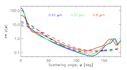
Figure 5: Scattering phase function for mode 1 (dashed) and mode 2 (solid) haze at selected wavelengths. A scattering angle of zero corresponds to the forward scattering direction. For a color version of the figure, see the electronic journal.

Mode 1 haze is characterized by $r_{g}$=0.15 $\mu$m and $\sigma_{g}$=1.5 (effective radius and variance of $r_{\rm{eff}}$=0.23 $\mu$m and $v_{\rm{eff}}$=0.18, respectively), and a number density profile that drops with the background pressure as 900$\times$$p$/$p(60\;\rm{km})$ cm^-3. For mode 2 haze, $r_{g}$=1.0 $\mu$m, $\sigma_{g}$=1.21 ($r_{\rm{eff}}$=1.09 $\mu$m and $v_{\rm{eff}}$=0.037), and the number density profile is 120$\times$$p$/$p(60\;\rm{km})$ cm^-3. For our simulations, we extended indefinitely upwards the $p$/$p(60\;\rm{km})$ profile. Indeed, mode 1 particles are long known to exist above 80 km, and two works (Wilquet et al., wilquetetal2009 (2009); de Kok et al., dekoketal2011 (2011)) recently identified sizeable amounts of mode 2 particles up to 90–95 km. Both $r_{\rm{eff}}$ and $v_{\rm{eff}}$ are defined by Hansen & Travis (hansentravis1974 (1974)). Note, though, that the definition of $\sigma_{g}$ in that work corresponds to $\ln{\sigma_{g}}$ here. We assessed that the effect of extending the aerosol profile above 100 km was negligible because the aerosol layer becomes effectively thin at such altitudes. The wavelength-dependent cross sections, albedos and scattering phase functions for each mode are calculated from Mie theory (Mishchenko et al., mishchenkoetal2002 (2002)). The complex refractive indices for the aerosol particles (H₂SO₄/H₂O solutions at 84.5% by weight, Molaverdikhani et al. (molaverdikhanietal2012 (2012))) were borrowed from Palmer & Williams (palmerwilliams1975 (1975)). Figure (4) graphs the extinction profile at 60 km from 0.2 to 5 $\mu$m, that appears to be dominated by mode 2 particles. Figure (5) shows the scattering phase function of each mode at specific wavelengths.

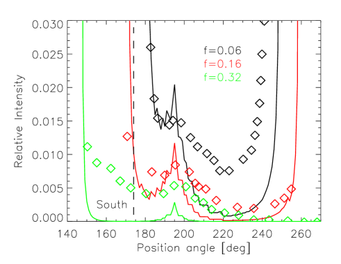
Figure 8: Relative intensity against position angle from G-band observations (symbols) at the Dutch Open Telescope on La Palma (Spain) and modelling in this work at 0.43 $\mu$m (solid) for the egress during the 2004 Venus transit. The intensities and position angle are defined by Tanga et al. (tangaetal2012 (2012)). To reproduce the peak in brightness away from the South Pole, we needed to shift the reference $h_{\rm{cloud}}$–latitude profile by about 20^∘. For a color version of the figure, see the electronic journal.

The aerosol profile based on Molaverdikhani et al. (molaverdikhanietal2012 (2012)) reaches $\tau_{\rm{nadir}}$=1 at 1.6 $\mu$m near 70 km, which may represent a globally-averaged cloud top altitude. A limb opacity $\tau_{\rm{limb}}$=1 is reached about 4–5 scale heights higher and therefore likely above 85 km. This globally-averaged description is correct to first order, but the appropriate simulation of the halo requires a more accurate characterization of latitudinal variations in the cloud top level. Recent altimetry of the Venus clouds from Venus Express shows that $\tau_{\rm{nadir}}$=1 is reached at about 74 km near the equator but may drop to 64 km at the poles, with transition zones on both hemispheres at about 60^∘ latitude (Ignatiev et al., ignatievetal2009 (2009)). To account for this latitudinal dependence, we shifted at each latitude the aerosol profiles upwards or downwards as needed to match the cloud top altitudes graphed in Fig. 8b of Ignatiev et al. (ignatievetal2009 (2009)).

3 The halo

The halo (or aureole) is the refracted image of the Sun that forms at the planet’s outer terminator for small Sun-Venus angular separations, with possibly a minor contribution from diffuse sunlight. Its appearance is determined by the geometrical configuration of the two objects relative to the observer and by the optical properties of the Venus stratified atmosphere. This section addresses the visual phenomenon as contemplated from a geocentric vantage point for the conditions of the June 2012 transit. The geometrical parameters needed in the simulations are either adopted or inferred from the JPL HORIZONS service (Giorgini et al., giorginietal1996 (1996)) or the New Horizons GeoViz software.

3.1 Some geometrical considerations

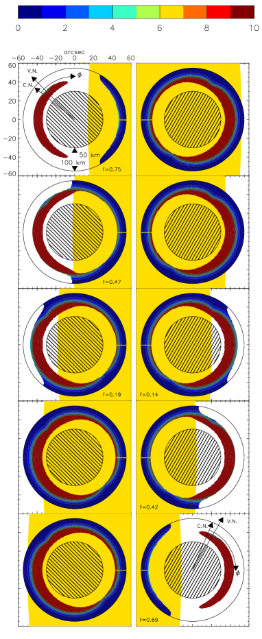
Figure 6: Isolines of $\Phi$=$-\log_{10}(L_{D}\mathbf{(x_{O},s_{O})}/B_{\odot})$ at 0.55 $\mu$m during ingress and egress. The Venus solid core plus atmosphere up to 50 km are represented to scale in dashed fill. The atmospheric ring from 50 to 100 km has been resized for a better appreciation of the halo’s structure. The atmosphere above 100 km is not shown. The unrefracted view of the solar disk is shown to scale in yellow in the background. The directions for the Venus North Pole and the Celestial North are indicated. Also indicated is the azimuthal angle $\phi$ as defined in Figs. (7)–(9). In the color code of the figure, blue indicates bright and brown indicates faint. For a color version of the figure, see the electronic journal.

Figure (6) shows a sequence of simulations of both the ingress and the egress. Each simulation corresponds to a value for the $f$ factor introduced by Link (link1969 (1969)) and used by Tanga et al. (tangaetal2012 (2012)). This factor stands for the fraction of the planet’s diameter along the Venus-Sun line of centres beyond the Sun’s limb. Thus, $f$= 1, 0.5 and 0 are appropriate for external contact, mid-ingress/-egress and internal contact, respectively. For a better visualization, the atmospheric ring from 50 to 100 km altitude is stretched by a fixed factor in all images. Ignoring for the time being the sunlight extinction caused by the gas and haze, the Sun’s image at the planet’s outer terminator appears notably diminished with respect to the apparent size of the unocculted solar disk. The diminishment constitutes the visual representation of the attenuation by refraction.

Referring to Table (1), the deflected angle for rays crossing the atmosphere with an impact distance $r_{b}$$-$$R_{\venus}$=55 km is $\alpha_{\rm{refr}}$$\sim$1^∘, thus exceeding the solar angular diameter as viewed from Venus ($\sim$2$R_{\odot}$/0.726 AU$\sim$0.734^∘). This means that, in geometrical terms, the halo representations of Fig. (6) are the refracted images of the entire solar hemisphere visible from Venus. The innermost/outermost contours are the projections of the farther/closer edges of the solar disk, respectively.

The bottom left and top right images of Fig. (6) show the planet shortly after contact II and before contact III, respectively. At those instants the atmosphere does not form a refracted image at the inner terminator below $\sim$76 km on the axis between the centres of the two objects. At the outer terminator, a refracted image occurs only above $\sim$59 km. This asymmetry is caused by the unequal distance from each terminator to the opposite solar limb. The oval ring within which a solar image is not formed dictates the range of atmospheric altitudes that cannot be accessed from Earth regardless of atmospheric opacity. This refraction exclusion ring becomes circular as the planet moves towards mid-transit.

3.2 Shape and brightness of the halo

The simulations of Fig. (6) assume a continuum wavelength of 0.55 $\mu$m and the latitude-dependent extinction coefficient described in §2.4. To take into account the varying altitude of clouds along the terminator, we solved the RTE over the entire Venus disk for a range of $h_{\rm{cloud}}$ values and, subsequently, composed the displayed images by assembling the relevant latitude–$h_{\rm{cloud}}$ sectors.

Venus enters the transit with its rotational axis tilted by about 45^∘ clockwise with respect to the Venus-Sun line of centres. At egress, the tilt is about 60^∘ and anticlockwise. The tilts were estimated graphically from GeoViz simulations. In combination, the inclination of the rotational axis and the latitude-dependent altitude of the cloud tops break the symmetry of the halo expected from purely geometrical arguments. The asymmetry is clearly discerned in the contours of Fig. (6), each of them corresponding to a value for $\Phi$=$-\log_{10}(L_{D}\mathbf{(x_{O},s_{O})}/B_{\odot})$.

At ingress, the earliest evidence of the halo occurs over the Venus North Pole and appears detached from the solar disk until about mid-ingress. The bright cap finally turns into a full ring that encircles the planet before contact II. Essentially, the egress reproduces the ingress sequence in the reverse order. During egress, the larger tilt of the rotational axis causes the halo to appear attached to the solar disk for a longer duration.

Figure (6) provides insight into the instantaneous vertical extent of the halo. Importantly, the halo’s outermost contour remains confined to altitudes less than 100 km for most of the ingress/egress. The statement is easily verified with a quick estimate specific to the instant halfway through ingress/egress. At that moment, a ray emanating from the nearer solar limb and propagating on the azimuthal plane that includes the Venus-Sun line of centres must be deflected by an angle $\sim$$R_{\venus}$/0.726 AU+$R_{\venus}$/0.274 AU$\approx$42 arc sec to reach the geocentric observer. Refraction yields such a deflection at $\sim$80 km altitude, as seen in Table (1). Thus, at mid-ingress or -egress only rays traced from $\mathbf{x_{O}}$ on the plane containing the line of centres with $r_{b}$ less than that may connect the observer and the solar disk.

The conclusion serves to highlight the importance of haze on the halo’s changing appearance because the atmosphere is likely optically thick in limb viewing at those altitudes. The halo’s inner contour is largely dictated by extinction in the optically thicker layers of the atmosphere. Overall, the altitudes contributing effectively to the halo range over 1–2 scale heights.

3.3 The imaged solar disk

It is interesting to trace the rays forming the halo back to the solar surface elements they departed from. In geometrical terms, the halo is the refracted image of most of the solar disk visible from Venus or Earth. However, haze extinction concentrates the rays effectively contributing to the halo’s brightness onto a narrow strip near the solar limb. Our ray tracing scheme does indeed show that during ingress/egress the halo is essentially formed by the solar disk occulted behind Venus. That solar region is severely limb-darkened, which adds a significant radial gradient to the solar output brightness. In the serendipitous situation that a dark sunspot is occulted by the planet during ingress/egress, one may expect that the sunspot will turn up as a dimmer halo.

3.4 Chromaticity of the halo and limb-integrated lightcurves

The halo’s shape and brightness depend on the atmospheric refractivity, sunlight extinction and solar limb-darkening. In turn, these factors depend on wavelength. Focusing on the visible and near-infrared regions of the spectrum, we investigated them at 0.43, 0.55 and 0.8 $\mu$m, which roughly match the center wavelengths of the B, V and I filters, respectively.

The refractivity of the Venus atmosphere varies with wavelength, which may introduce a relative displacement between the images formed at different colors. Considering again Fig. (2), we can devise two rays of wavelengths $\lambda_{1}$ and $\lambda_{2}$ departing from a common solar surface element, both of them reaching the observer. Since the overall deflections are nearly identical, we can readily estimate their altitudes of closest approach in the atmosphere. According to the approximate, analytical formula given by Baum & Code (baumcode1953 (1953)) for the refraction angle in an isothermal atmosphere, the number densities at closest approach of the two rays are in the ratio $n_{1}$/$n_{2}$$\sim$$\nu_{\lambda_{2}}$/$\nu_{\lambda_{1}}$, with $\nu$ being the refractivity at the specified wavelength. For Venus, this means that if $\lambda_{1}$=0.43 and $\lambda_{2}$=0.8 $\mu$m the rays have their closest approach at densities in the ratio $n_{1}$/$n_{2}$$\sim$0.9747. For an atmospheric scale height of 4 km, this means that the altitudes of closest approach differ by about one hundred meters. Thus, the displacement of the images due to refraction is relatively minor.

Haze dominates the atmospheric opacity from the UV to the NIR at the altitudes of formation of the halo. Recalling from Fig. (4) the spectral dependence of $\gamma(\mathbf{x})$, it is apparent that the sunlight emerging from the Venus terminator must exhibit a moderate red tone imprinted by haze extinction. The reddening is, however, much less than expected for a Rayleigh atmosphere, in which case $\gamma(\mathbf{x})$$\sim$$\lambda^{-4}$. Sunlight emitted from the solar limbs is eminently red, as seen in Fig. (1). Thus, solar limb darkening must also contribute towards the reddening of the halo.

To study this in a quantitative manner, we produced radially-averaged radiances of the halo as follows:

$$\langle\frac{L_{D}(\bf{x_{O}},\bf{s_{O}})}{B_{\odot}}\rangle=\frac{\int\limits_{\mu_{M}}^{\mu_{m}}\!L_{D}(\bf{x_{O}},\bf{s_{O}})/\rm{\it{B}_{\odot}}\,\it{d}(\mu^{2}/2)}{\int\limits_{\mu_{M}}^{\mu_{m}}{d}(\mu^{2}/2)}=\int\limits_{0}^{1}\!{\frac{L_{D}(\xi,\eta)}{B_{\odot}}}\,\it{d}\xi$$ (7)

which is equivalent to averaging over altitude from the ground to 200 km or over 1 arcsec for ground-based observations. Thus, $<$${{{L_{D}}}}({\bf{x_{O}}},{\bf{s_{O}}})/B_{\odot}$$>$ is a valid measure of the vertically-unresolved brightness with respect to the brightness at the Sun’s centre.

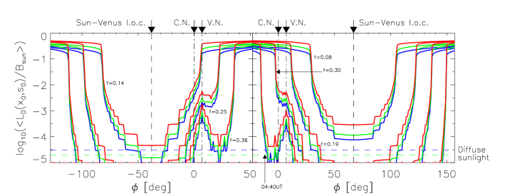
Figure 7: Limb-integrated lightcurves during ingress and egress at 0.43 (blue), 0.55 (green) and 0.8 (red) $\mu$m. Reference $h_{\rm{cloud}}$–latitude profile. For a color version of the figure, see the electronic journal.

Curves of the radially-averaged radiance for $\lambda$=0.43, 0.55 and 0.8 $\mu$m during ingress and egress are graphed against the azimuthal angle $\phi$ in Fig. (7). The curves show a strong time-dependence and reveal with an increased brightness the lower clouds occurring at the Venus North Pole. The color dependence of the lightcurves near the Sun-Venus line of centres is due to both solar limb darkening and atmospheric sunlight extinction. Close to the solar disk edge (the left and right pedestals of the figure), the higher atmospheric altitudes contribute significantly and only solar limb darkening introduces a color dependence.

These curves constitute a direct target for comparison with photometric measurements. Indeed, Tanga et al. (tangaetal2012 (2012)) recently published limb-integrated curves from observations of the 2004 transit. Figure (8) shows with symbols their G-band lightcurves obtained during egress at the Dutch Open Telescope on La Palma as digitized from their Fig. 8. Relative intensities are represented against the azimuthal angle and reveal the expected U shape as well as a peak in brightness displaced from the pole. The solid curves are our model lightcurves at 0.43 $\mu$m for the 2004 egress conditions. Tanga et al. (2012) normalize their lightcurves with the solar disk brightness at about one Venus radius from the solar edge. For consistency, we re-scaled our radially-averaged radiances by the appropriate limb-darkening factor, so that the two sets of curves become directly comparable. The comparison for three different instants during egress is overall satisfactory, especially taking into account that we assumed a global description for the cloud top altitude. Importantly, to achieve such an agreement, we needed to offset the location of the minimum cloud top altitude by about 20^∘ away from the pole. If confirmed, that feature might indicate that occasionally the cloud top altitude does not descrease monotonically with latitude towards the poles.

Following the comparison with Tanga et al. (2012), that work reports that as factor $f$ increases the halo brightness decays more rapidly at red wavelengths than at visible and ultraviolet wavelengths. As discussed earlier, our model predicts an overall red halo, which is somewhat at odds with the Tanga et al. (2012) findings. At any rate, the amplitude of the error bars in their experiment might also accomodate a small reddening. New observations of the 2012 transit will hopefully provide a better insight into the issue.

One may consider to use model lightcurves such as those in Fig. (7) to fit the empirical lightcurves and retrieve cloud altitudes along the planet’s terminator. Tanga et al. (tangaetal2012 (2012)) have already approached the task. To understand to what extent the model lightcurves depend on the prescribed atmospheric optical properties, we produced limb-integrated lightcurves with the cloud top altitude shifted at all latitudes by $\pm$1 km with respect to the reference cloud altimetry. The resulting lightcurves are given in Fig. (9) and show that shifting the cloud tops by $\pm$1 km leads to variations in the limb-averaged radiances by factors of $\sim$2 or more. Ultimately, the precision of the method to retrieve the cloud top altitude will depend strongly on the quality of the photometric data. Spatial resolution in the data is not anticipated to be critical, since resolutions of about 1 arcsec are commonly achieved also from ground-based observatories. A cadence of one image per minute or less suffices to reveal the temporal evolution of the lightcurves.

Some observers of the 2012 Venus transit may also attempt the spectroscopic characterization of the halo. The likely result of such an experiment will be similar to a transmission spectrum of the Venus atmosphere from an altitude of 85 km or higher with a continuum dependent on wavelength through both haze extinction and solar limb darkening.

3.5 Diffuse sunlight contribution to the halo

One more issue to explore is the contribution of diffuse sunlight to the overall brightness of the halo. In between external and internal contacts, the Sun-Venus-Earth angle is more than $\sim$179^∘, which favors forward scattering from the planet’s terminator. Most atmospheric aerosols scatter efficiently in the forward direction, with the scattering efficiency depending strongly on the ratio $x_{\rm{eff}}$=2$\pi$$r_{\rm{eff}}$/$\lambda$ of the effective radius for the particle size distribution and the incident sunlight wavelength (Hansen & Travis, hansentravis1974 (1974)). As seen in Fig. (5), the peak in the scattering phase function becomes enhanced at the shorter wavelengths and is particularly stronger for the larger mode-2 haze.

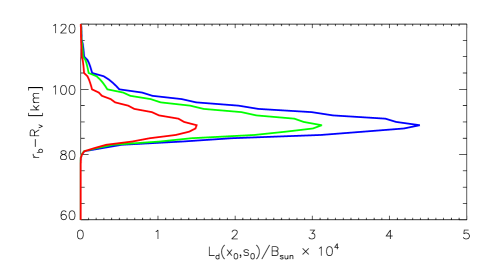
Figure 10: Diffuse radiance $L_{d}\mathbf{(x_{O},s_{O})}/B_{\odot}$ graphed against the impact radius $r_{b}-R_{\venus}$. From right to left, the curves correspond to wavelengths of 0.43, 0.55 and 0.8 $\mu$, respectively. For a color version of the figure, see the electronic journal.

Figure (10) graphs the multiple-scattering diffuse radiance at mid-transit (with the Sun, Venus and Earth perfectly aligned) against the impact radius as calculated with the Monte Carlo method of §2.3. For simplicity, we assumed that the cloud top lies at a constant altitude of 70 km at all latitudes. The radiances peak at $\sim$88 km, that corresponds approximately to the $\tau_{\rm{limb}}$=1 level. Shifting upwards/downwards the clouds by a few kilometers merely shifts the radiances by the same distance but has a negligible impact on the vertically-integrated magnitudes.

Integration of the curves in Fig. (10) results in radially-averaged diffuse radiances $<$$L_{d}\mathbf{(x_{O},s_{O})}/B_{\odot}$$>$ of $\sim$3$\times$10^-5, 2$\times$10^-5 and 1$\times$10^-5 at 0.43, 0.55 and 0.8 $\mu$m, respectively. Comparison with the lightcurves of Fig. (7) indicates that refracted sunlight dominates the halo’s brightness over most of the ingress/egress.

4 Venus-Sun disk-integrated lightcurves

We have thus far assumed that the Venus disk is spatially resolvable from Earth, a necessary condition to investigate the connection between the halo’s structure and the cloud altimetry along the planet’s terminator. However, the question of whether the atmospheric properties of a transiting planet can be disentangled from the planet-star blended signal has become key in the research of extrasolar planets (Seager & Sasselov, seagersasselov2000 (2000); Brown, brown2001 (2001); Hubbard et al., hubbardetal2001 (2001)).

The so-called technique of transits aims to identify the signatures of the planet and its atmosphere from comparative measurements of the planet-star light out of and in transit. In-transit spectroscopy (or spectrophotometry) is providing valuable insight into exoplanetary atmospheres, especially for the giant planets that constitute most of the exoplanet detections to date. As the sizes of discovered extrasolar planets shrink and technology improves, the prospects for characterizing Earth-sized planets with this technique, including Venus-like ones, look closer. Next, we describe the Venus transit as if observed in integrated light from a terrestrial distance and from a remote vantage point.

4.1 Disk-integrated lightcurves from Earth and far away

Figure (11) shows model transit depths at 0.55 $\mu$m for the Venus-Sun system as observed from Earth. The transit depths are expressed in units of irradiance for the unobstructed Sun. The overall shape of the lightcurve is determined by the ratio of Venus/Sun solid angles, $\sim$1/30, and the limb darkening function at the specified wavelength.

Refraction introduces unique features in the lightcurves near external and internal contacts. In Fig. (11), we show also the difference in transit depths when refraction is taken into account and when it is omitted. If the Venus atmosphere was free of haze and cloud particles, the differential transit depth curve would show that the planet’s size is determined by a combination of Rayleigh scattering and refraction. A refraction exclusion ring appears at altitudes from $\sim$59 to $\sim$76 km, depending on the distance from the planet’s local terminator to the solar limb, and contributes most significantly to the disk-integrated lightcurve near internal contact. Note also that the depth varies by $\sim$3$\times$10^-7 from mid-transit to internal contact, which means that the planet’s measurable radius apparently expands by a few km. Out of transit, the transit depth inverts its sign because sunlight refracted by the planet contributes positively to the brightness of the Venus-Sun system. The magnitude of this additional brightening amounts to $\sim$7$\times$10^-7 at external contact. Including haze in the calculation of the optical opacity reduces by orders of magnitude the effects of refraction in the differential transit depths, as the dotted curve in the figure indicates. At any rate, such small perturbations fall well below typical irradiance fluctuations due to solar oscillations over periods of minutes (Kopp et al., koppetal2005 (2005)).

The disk-integrated lightcurves measured by a remote observer would exhibit the same phenomena described above. The considerably smaller ratio of Venus/Sun solid angles in that case, $\sim$$R_{\venus}/R_{\odot}$$\sim$1/115, would cause the same phenomena to appear about one order of magnitude fainter in the combined planet-star signal. Figure (12) demonstrates the disk-integrated lightcurves in the limit of an infinitely distant observer.

4.2 Disk-integrated transmission spectra

The monochromatic lightcurves presented in §4.1 might also be calculated at wavelengths exhibiting discrete molecular absorption features. We produced spectra for the transit depth at wavelengths from about 0.3 to 5 $\mu$m. In addition to CO₂, the atmosphere was assumed to contain small amounts of N₂, CO and O (Vandaele et al., vandaeleetal2008 (2008); Hedin et al., hedinetal1983 (1983)) and H₂O (1 ppm; Fedorova et al., fedorovaetal2008 (2008)). The line parameters for molecular transitions were borrowed from HITRAN 2008 (Rothman et al., rothmanetal2009 (2009)). The transit depths were degraded to a resolving power of about 10³ and expressed in terms of the equivalent height. (The equivalent height is the height of an opaque slab that would produce an identical transit depth.) In equivalent heights, the spectra measured from Earth and from a remote distance are nearly identical, yet the associated stellar dimming may differ by an order of magnitude. Whether observed from Earth ($d_{\rm{\bf{O}}}$/$l_{\odot}$$\sim$0.274) or from a remote distance ($d_{\rm{\bf{O}}}$/$l_{\odot}$$\sim$1), the solar irradiance blocked by the Venus disk and atmosphere is $F_{d+a}$$\sim$$\pi((R_{\venus}+h_{\rm{eq}})/d_{\rm{\bf{O}}})^{2}$$B_{\odot}$$U(\mu_{\odot})$, where we tacitly assume that the planet is nearly point-like and the background solar radiance is determined by a single $\mu_{\odot}$ dependent on the planet’s phase. In relative terms, the solar dimming during transit is $F_{d+a}$/$F_{\odot}$.

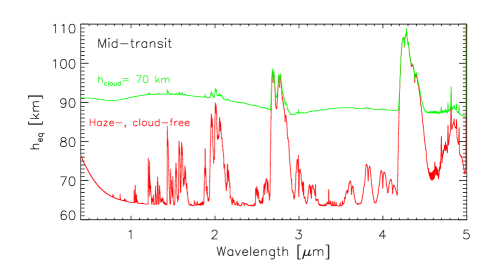
Figure 13: Mid-transit transmission spectrum of Venus at a resolving power of 10³ in two different atmospheric conditions. For a color version of the figure, see the electronic journal.

The curves in Fig. (13) correspond to mid-transit ($\mu_{\odot}$=1) spectra calculated for an atmosphere free of haze and cloud particles and for a hazy atmosphere with cloud tops at 70 km. The latter seems to reproduce most of the structure of the in-transit spectrum presented by Ehrenreich et al. (ehrenreichetal2012 (2012)). The most obvious difference between the Rayleigh and hazy atmospheres refers to the continuum level, that lies considerably higher in the latter. For the Rayleigh atmosphere, the continuum level is largely determined by refraction at wavelengths longer than $\sim$1 $\mu$m, with Rayleigh scattering contributing shortwards of that. For the hazy atmosphere, the continuum is dictated by the haze optical properties throughout the spectrum. The simulations for phases other than mid-transit (not shown) indicate that for the Rayleigh atmosphere the transit depth of molecular bands is highest at mid-transit and a few kilometers less when the planet is near contacts. This modulation is attributable to refraction, and becomes entirely negligible for the hazy atmosphere.

The comparison is relevant because to some extent a clear-atmosphere Venus would be akin to our own Earth. Regarding the molecular structure of the spectra, it is overwhelmingly dominated by rovibrational bands of CO₂. Benneke & Seager (bennekeseager2012 (2012)) have investigated what can unambiguously be inferred from in-transit spectroscopy of a super-Earth, and noted that the lacking evidence of Rayleigh scattering may impede the identification of the main atmospheric constituent. Interestingly, it appears that the in-transit spectrum of Venus would reveal little on the identity of the main atmospheric constituent.

A final comment on the SO₂ molecule. The SO₂ molecule plays a key role in the Venus photochemistry and in the formation of H₂SO₄ in the clouds (Mills & Allen, millsallen2007 (2007)). The SO₂ molecule absorbs at wavelengths below $\sim$0.32 $\mu$m, at the limit of accessibility for ground-based observations imposed by the terrestrial ozone cut-off at $\sim$0.3 $\mu$m. Belyaev et al. (belyaevetal2012 (2012)) have retrieved the SO₂ mixing ratio for altitudes below 105 km. The precise amounts appear to be sensitive to the retrieval approach, which leads to values somewhere between 10^-7 and 10^-6 at altitudes above the $\tau_{\rm{limb}}$=1 level of $\sim$90 km. Figure (14) shows the equivalent height near 0.3 $\mu$m at high resolving power for SO₂ mixing ratios of 10^-7 and 5$\times$10^-7. The main conclusion to obtain from the graph is that SO₂ introduces a distinct signature that might be captured in spectroscopic observations of the transit if enough signal-to-noise ratio is achieved.

5 Summary

The current work presents theoretical insight into the signature imprinted on sunlight by the Venus atmosphere during the passage of the planet in front of the solar disk. The conclusions are specific to the June 2012 event but are easily generalizable to other transits. Our model approach includes refraction, multiple scattering and extinction by gases and aerosols in the atmosphere, as well as solar limb darkening, and handles all phases of the transit (including the out-of-transit, ingress/egress and in-transit stages) in a consistent manner. To the best of our knowledge this is the first theoretical investigation of the Venus transit at this level of detail.

We investigated the halo that forms at the planet’s outer terminator near ingress/egress, predicting its shape, brightness and chromaticity. Both the inner and outer contours of the halo are considerably affected by haze in the atmosphere above the clouds and below 100 km. The impact of haze opacity on the halo structure explains the variability of halo patterns from ingress to egress and from event to event. We estimated that scattered sunlight contributes less than refracted sunlight for most of the ingress/egress between internal and external contacts. Since our predictions are based on a realistic description of the Venus atmosphere it should be possible to verify them provided that accurate measurements become available. Further, our formulation opens a way for the characterization of the Venus atmosphere from observations during the transit. In retrospective, it is fair to state that if the Venus haze extended for 2–3 scale heights higher than it does, it is likely that the identification of a Venus atmosphere in the 18th century would have to have waited longer.

We presented lightcurves for the combined Venus-Sun signal during transit and discussed some features of the lightcurves associated with refraction. We also presented model in-transit spectra of Venus and of a haze- and cloud-free Venus-like planet. Haze appears recurrently as a key element in the interaction of sunlight and the Venus atmosphere. The disparate vertical extent of aerosols in their atmospheres establishes a considerable difference between Venus and Earth. Had the proper technology existed, it might have been appropriate to investigate the historic record of observed Venus transits. In this respect, the 2004 and 2012 events may set a valuable start point for comparisons between transits.

Finally, the Venus transit of 2012 arrives at a moment of great activity in the exploration of extrasolar planets by the method of transits. We have seen that high-altitude aerosols introduce specific challenges to the characterization of the atmospheric composition and cloud top altitude for a transiting Venus. Since it is still unknown how frequently high-altitude clouds may occur in the atmospheres of extrasolar planets, there are reasons to think that the challenges posed by Venus might also be generally encountered in the characterization of those planets. Indeed, recent work on hot Jupiter HD 189733b (Lecavelier des Etangs et al., lecavelierdesetangsetal2008 (2008); Huitson et al., huitsonetal2012 (2012)) and super-Earth GJ 1214b (Berta et al., bertaetal2012 (2012)) suggest that haze must be invoked to explain the appearance of their transmission spectra.

Table 1: Total refracted angles $\alpha_{\rm{refr}}$ for rays at 0.55 $\mu$m entering the atmosphere with an impact radius $r_{b}$. For comparison, $\alpha_{\rm{refr}}^{*}$ is the refracted angle for an isothermal atmosphere of refractivity $\nu_{\lambda=0.55\mu m}$ and scale height $H_{\rm{atm}}$ (Baum & Code, baumcode1953 (1953)).

$r_{b}-R_{\venus}$	$\nu_{\lambda=0.55\mu m}$	$H_{\rm{atm}}$	$\alpha_{\rm{refr}}$	$\alpha_{\rm{refr}}^{*}$
[km]		[km]	[arc sec]
55	2.12$\times$10-4	6.6	3794	3444
60	1.09$\times$10-4	5.6	2048	1852
70	1.82$\times$10-5	5.0	325	328
80	2.56$\times$10-6	4.5	45	48
90	2.65$\times$10-7	3.8	5.1	5.5
100	1.91$\times$10-8	3.8	0.45	0.39
110	1.47$\times$10-9	4.1	0.036	0.029
120	1.26$\times$10-10	4.3	0.0030	0.0024
$\alpha_{\rm{refr}}^{*}$= $\nu_{\lambda=0.55\mu m}$$\sqrt{2\pi R_{\venus}/H_{\rm{atm}}}$.

Figure 2: Sketch of the Venus-Sun system at an instant near internal contact. The rays traced from ${\bf{{x_{O}}}}$ fan out as they traverse the Venus stratified atmosphere.

Figure 3: The sketch demonstrates how a differential element of solid angle $d\Omega$ fans out when traced sunwards from the observer’s site. The dashed line represents the trajectory passsing through the middle-point of the solid angle element. In a transparent atmosphere, the ratio of radiance and the squared refraction index is conserved on the ray trajectory, and the corresponding irradiance for the differential solid angle element is simply ${{L}}({\bf{x_{O}}},{\bf{s_{O}}}){{\bf{s_{O}}}\cdot{\bf{n_{x_{O}}}}}d{\Omega(\bf{s_{O}})}$$\sim$ ${{L}}({\bf{x_{\odot}}},{\bf{s_{\odot}}})d{\Omega(\bf{s_{O}})}$. For the calculation of Eq. (3), a mathematical transformation is applied to rewrite the integral in the the auxiliary variables $\xi$ and $\eta$.

Figure 4: Haze extinction coefficient at 60 km for cloud top at 70 km. At other altitudes, $\gamma(\lambda;z)$=$\gamma(\lambda;60\;\rm{km})$$\times$$p/p(60\;\rm{km})$.

Figure 9: Limb-integrated lightcurves at 0.55 $\mu$. Each pair of curves corresponds to the lightcurves obtained from perturbing the reference $h_{\rm{cloud}}$–latitude profile by $\pm$1 km.

Figure 11: Transit depths for the Venus-Sun integrated signal as observed from Earth. The dashed curves represent the differential transit depth contributed by refraction.

Figure 12: Same as Fig. (11) with the observer at an infinite distance.

Figure 14: Equivalent height for altitude-independent SO₂ mixing ratios of 1$\times$ and 5$\times$10^-7. The SO₂ absorption cross sections are from Blackie et al. (blackietal2011 (2011); 2011b )

- (1) Ambastha, A., Ravindra, B., & Gosain, S. 2006, Solar Phys., 233, 171
- (2) Barth, C. A. 1969, Appl. Opt., 8, 1295
- (3) Bates, D. R. 1984, Planet. Space Sci., 32, 785
- (4) Baum, W. A., & Code, A. D. 1953, Astron. J., 58, 108
- (5) Belyaev, D. A., Montmessin, F., Bertaux, J.-L., Mahieux, A., Fedorova, A. A., Korablev, O. I. et al. 2012, Icarus, 217, 740
- (6) Benneke, B. & Seager, S. 2012, Astrophys. J., 753, 100
- (7) Ben-Abdallah, P., Le Dez, V., Lemonnier, D., Fumeron, S. ,& Charette, A. 2001, JQSRT, 69, 61
- (8) Berta, Z. K., Charbonneau, D., Désert, J.-M., Miller-Ricci Kempton, E., McCullough, P. R. et al. 2012, Astrophys. J., 747, 35
- (9) Blackie, D., Blackwell-Whitehead, R., Stark, G., Pickering, J. C., Smith, P. L., et al. 2011, J. Geophys. Res., 116, E03006, doi:10.1029/2010JE003707
- (10) Blackie, D., Blackwell-Whitehead, R., Stark, G., Pickering, J. C., Smith, P. L., et al. 2011b, J. Geophys. Res., 116, E12099, doi:10.1029/2011JE003977
- (11) Brown, T. M. 2001, Astrophys. J., 553, 1006
- (12) Claret, A. 2000, A&A, 363, 1081
- (13) de Kok, R., Irwin, P. G. J., Tsang, C. C. C., Piccioni, G., & Drossart, P. 2011, Icarus, 211, 51
- (14) Ehrenreich, D., Vidal-Madjar, A., Widemann, T., Gronoff, G., Tanga, P., Barthélemy, M., Lilensten, J., Lecavelier des Etangs, A.,& Arnold, L. 2012, A&A Lett., 537, L2
- (15) Énomé, S. 1969, PASJ, 21, 367
- (16) Esposito, L. W., Knollenberg, R. G., Marov, M. Y., Toon, O. B., & Turco, R. P. 1983, in Venus, ed. D. M. Hunten, L. Colin, T. M. Donahue, & V. I. Moroz (Univ. of Arizona Press, Tucson) 484
- (17) Fedorova, A., Korablev, O., Vandaele, A.–C., Bertaux, J.–L., Belyaev, D., et al. 2008, J. Geophys. Res., 113, E00B22
- (18) Fumeron, S., Charette, A., & Ben-Abdallah, P. 2005, JQSRT, 95, 33
- (19) García Muñoz A. & Pallé E. 2011, JQSRT, 112, 1609
- (20) García Muñoz, A., Pallé, E., Zapatero Osorio, M. R., Martín, E. L. 2011, Geophys. Res. Lett., 38, L14805
- (21) García Muñoz, A., Zapatero Osorio, M. R., Barrena, R., Montañés-Rodríguez, P., Martín, E. L., Pallé, E. 2012, Astrophys. J., 755, 103
- (22) Giorgini, J. D., Yeomans, D. K., Chamberlin, A. B., Chodas, P. W., Jacobson, R.A., et al., 1996, BAAS, 28, 1158.
- (23) Hansen, J. E. & Travis, L. D. 1974, Space Science Reviews, 16, 527
- (24) Hays, P. B. & Roble, R. G. 1968, J. Atmos. Sciences, 25, 1141
- (25) Hedelt, P., Alonso, R., Brown, T., Collados Vera, M., Rauer, H., Schleicher, H., Schmidt, W., Schreier, F. & Titz, R. 2011, A&A, 533, A136
- (26) Hedin, A. E., Niemann, H. B., Kasprzak, W. T. & Seiff, A. 1983, J. Geophys. Res., 88, 73
- (27) Hestroffer, D. & Magnan, C. 1998, A&A, 333, 338
- (28) Hubbard, W. B., Fortney, J. J., Lunine, J. I., Burrows, A., Sudarsky, D. & Pinto, P. 2001, Astrophys. J., 560, 413
- (29) Huitson, C. M., Sing, D. K., Vidal-Madjar, A., Ballester, G. E., Lecavelier des Etangs, A., et al. 2012, MNRAS, 422, 2477
- (30) Ignatiev, N. I., Titov, D. V., Piccioni, G., Drossart, P., Markiewicz, W. J., Cottini, V., Roatsch, Th., Almeida, M & Manoel, N. 2009, J. Geophys. Res., 114, E00B43, doi:10.1029/2008JE003320
- (31) Kopp, G., Lawrence, G. & Rottman, G. 2005, Solar Phys., 230, 129
- (32) Kowalski, P. M.,& Saumon, D. 2004, Astrophys. J., 607, 970
- (33) Lecavelier des Etangs, A., Pont, F., Vidal-Madjar, A., & Sing, D. K. 2008, A&A, 481, L83
- (34) Link, F. 1959, Bull. Astron. Inst. Czechoslovakia, 10, 105
- (35) Link, F. 1962, in Physics and Astronomy of the Moon, ed. Z. Kopal, 161
- (36) Link, F. 1969, Eclipse phenomena in astronomy (Springer-Verlag, Berlin Heidelberg) 205–225
- (37) Mayor, M., & Queloz, D. 1995, Nature, 378, 355
- (38) Mills, F. P., & Allen, M. 2007, Planet. Space Sci., 55, 1729
- (39) Mishchenko, M. I., Travis, L. D.,& Lacis, A. A. 2002, Scattering, absorption and emission of light by small particles (Cambridge University Press, Cambridge)
- (40) Molaverdikhani, K., McGouldrick, K., & Esposito, L. W. 2012, Icarus, 217, 648
- (41) O’Brien, D. M. 1992, JQSRT, 48, 41
- (42) Old, J. G., Gentili, K. L., & Peck, E. R. 1971, J. Opt. Soc. Am., 61, 89
- (43) Palmer, K. F., & Williams, D. 1975, Appl. Opt., 14, 208
- (44) Pasachoff, J. M., Schneider, G.,& Widemann, T. 2011, Astron. J., 141, 112
- (45) Pasachoff, J. M. 2012, Nature, 485, 303
- (46) Pierce, A. K. & Slaughter, C. D. 1977, Solar Phys., 51, 25
- (47) Pierce, A. K., Slaughter, C. D. & Weinberger, D. 1977, Solar Phys., 52, 179
- (48) Pollack, J. B., Toon, O. B., Whitten, R. C., Boese, R., Ragent, B., et al. 1980, J. Geophys. Res., 85, 8141
- (49) Rothman, L. S., Gordon, I. E., Barbe, A., Benner, D. C., Bernath P. F., et al. 2009, JQSRT, 110, 533
- (50) Seager, S., & Sasselov, D. D. 2000, Astrophys. J., 537, 916
- (51) Seager, S. & Deming, D. 2010, Annu. Rev. Astron. Astrophys., 48, 631
- (52) Seiff, A., Schofield, J. T., Kliore, A. J., Taylor, F. W., Limaye, S. S., et al. 1985, Adv. Space Res., 5, 3
- (53) Schneider, G., Pasachoff, J. M., & Golub, L. 2004, Icarus, 168, 249
- (54) Schneider, G., Pasachoff, J. M., & Willson, R. C. 2006, Astrophys. J., 641, 565
- (55) Sidis, O., & Sari, R. 2010, Astrophys. J., 720, 904
- (56) Sing, D. K. 2010, A&A, 510, A21
- (57) Tanga, P. Widemann, T., Sicardy, B., Pasachoff, J. M., Arnaud, J. et al. 2012, Icarus, 218, 207
- (58) Vandaele, A. C., De Mazière, M., Drummond, R., Mahieux, A., Neefs, E. et al. 2008, J. Geophys. Res., 113, E00B23
- (59) van der Werf, S. Y. 2008, Appl. Opt., 47, 153
- (60) Wilquet, V., Fedorova, A., Montmessin, F., Drummond, R., Mahieux, A. et al. 2009, J. Geophys. Res., 114, E00B42
- (61) Zheleznyakov, V. V. 1967, Astrophys. J., 148, 849