Throughflow centrality is a global indicator of the functional importance of species in ecosystems

Abstract

To better understand and manage complex systems like ecosystems it is critical to know the relative contribution of the system components to the system function. Ecologists and social scientists have described a diversity of ways that individuals can be important; This paper makes two key contributions to this research area. First, it shows that throughflow ($T_{j}$), the total energy or matter entering or exiting a system component, is a global indicator of the relative contribution of the component to the whole system activity. Its global because it includes the direct and indirect exchanges among community members. Further, throughflow is a special case of Hubbell status or centrality as defined in social science. This recognition effectively joins the concepts, enabling ecologists to use and build on the broader centrality research in network science. Second, I characterize the distribution of throughflow in 45 empirically-based trophic ecosystem models. Consistent with theoretical expectations, this analysis shows that a small fraction of the system components are responsible for the majority of the system activity. In 73% of the ecosystem models, 20% or less of the nodes generate 80% or more of the total system throughflow. Four or fewer nodes are required to account for 50% of the total system activity and are thus defined as community dominants. 122 of the 130 dominant nodes in the 45 ecosystem models could be classified as primary producers, dead organic matter, or bacteria. Thus, throughflow centrality indicates the rank power of the ecosystems components and shows the concentration of power in the primary production and decomposition cycle. Although these results are specific to ecosystems, these techniques build on flow analysis based on economic input-output analysis. Therefore these results should be useful for ecosystem ecology, industrial ecology, the study of urban metabolism, as well as other domains using input-output analysis.

1 Introduction

Identifying functionally important actors is a critical step in understanding and managing complex systems, whether it is a fortune 500 company or an ecosystem. For example, Ibarra (1993) showed that an employee’s power to affect administrative innovation within an advertising agency was in part determined by their positional importance within the organization. In ecological systems, knowing the relative functional importance of species or groups of species is essential for conservation biology, ecosystem management, and understanding the consequences of biodiversity loss (Walker, 1992; Lawton, 1994; Hooper et al., 2005; Jordán et al., 2006; Saavedra et al., 2011).

Ecologists have several ways of classifying the relative importance of community members. Whittaker (1965) introduced rank–abundance curves to describe the community richness and indicate the relative importance of the species, assuming that community importance was proportional to abundance. He also presented an alternative rank–productivity curve that indicated the species importance based on their net productivity. Subsequent ecological concepts have built on this. Keystone species (Paine, 1966; Power et al., 1996) are species whose importance to the community are disproportionate to their biomass, like the sea otter in Pacific kelp forests. Ecological engineers (Lawton, 1994; Jones et al., 1994) are species whose actions create whole new habitats, such as beavers that transform terrestrial environments into slow moving aquatic environments. Dayton (1972) introduced the more general term foundational species for fundamentally important species of many types (Ellison et al., 2005). Part of the challenge and the reason for multiple concepts, is that there are a diversity of ways in which a species may be important and contribute to a community or ecosystem.

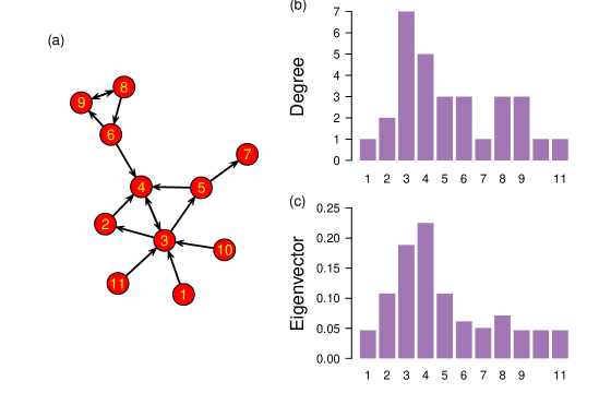
Figure 1: Hypothetical network model (a) with its associated (b) degree and (c) eigenvector centrality. Degree centrality is a local measure while eigenvector centrality is a global indicator of node importance.

Faced with the analogous problem of identifying important members of human communities, social scientists developed the centrality concept (see Wasserman and Faust, 1994). Centrality embodies the intuition that some community members are more important, have more power, or are more central to community function. Centrality was developed in the context of network models of communities in which individuals are represented as nodes of a graph and the graph edges signify a specific relationship between two individuals such as friendship or co-authorship (Fig. 1a). The relationship may or may not be directed. Degree centrality is the number of immediately adjacent neighbors on the graph, and it assumes that more connected nodes are more central. It is quantified as the number of edges incident to the node. In the example graph, node 3 has a degree of 7 (note the separate directed pathways from 3 to 4 and from 4 to 3 shown as a two headed arrow). Fig. 1b shows the distribution of node degrees in the community which indicates that node 3 is the most central from this local neighborhood perspective.

Some scientists have suggested that the local neighborhood is insufficient to determine the node’s centrality for some applications, especially exchange networks (Hubbell, 1965; Bonacich, 1972; Estrada, 2010). Instead, a node’s importance may be increased because one or more of its neighbors are important. Network models can capture this increased neighborhood size by defining a walk as a sequence of edges traveled from one node to another, and walk length ($m$) is the number of edges crossed. In the example network, there is a walk from 6 to 2 of length $m=3$ by following $6\rightarrow 4\rightarrow 3\rightarrow 2$. This enables us to consider the neighborhood $m$ steps aways (Estrada, 2010). Fig. 1c shows the eigenvector centrality (Bonacich, 1972, 1987) for the example network which identifies the equilibrium number of paths passing through each node as $m\rightarrow\infty$. In this sense it is a global centrality measure because it is a “summary of a node’s participation in the walk structure of the network” (Borgatti, 2005) and captures the importance of indirect as well as direct interactions (Borgatti, 2005; Scotti et al., 2007).

Degree and eigenvector are only two examples of centrality indicators. Many centrality measures have been developed and applied in the literature for complex systems modeled as networks (Wasserman and Faust, 1994; Koschützki et al., 2005). The centrality measures tend to be correlated (Newman, 2006; Jordán et al., 2007; Valente et al., 2008), but the differences can be informative (Estrada and Bodin, 2008; Baranyi et al., 2011). Borgatti and Everett (2006) provide a classification of centrality indices and shows how and why different measures are useful for different applications.

Ecologists have applied the centrality concept in several ways. For example, landscape ecologists have used centrality to assess the connectivity of habitat patches, how this connectivity effects organism movement, and how habitat loss changes the connectivity (Estrada and Bodin, 2008; Bodin and Saura, 2010; Baranyi et al., 2011). Community and ecosystem ecologists have developed and used centrality measures to study how organisms influence each other in transaction networks (Jordán et al., 2003; Allesina and Pascual, 2009; Fann and Borrett, 2012). Jordán et al. (2006) argue that mesoscale measures, between local and global centralities, are most useful for ecosystem studies because the impact of indirect effects tend to decay rapidly as they radiate through the system. Recent work used centrality indicators to determine important species in communities of mutualists (Martín González et al., 2010; Sazima et al., 2010). Collectively, this work shows how a range of centrality indicators can be useful for addressing ecological questions.

Here, I identify a new centrality indicator for ecology, termed throughflow centrality $T_{j}$. I first recognize that the throughflow measure ecosystems ecologists have long calculated (Patten et al., 1976; Finn, 1976; Ulanowicz, 1986) is a global measure of node importance in generating the total system activity. Further, I show that this is a special case of Hubbell’s status index centrality (Hubbell, 1965). I then apply this measure to 45 trophic ecosystem models drawn from the literature to test two hypotheses regarding ecosystem organization. The first hypothesis suggested by both Whittaker (1965) and Mills et al. (1993) is that communities are composed of a relatively few dominant species and larger group that are less central. The second hypothesis is that in ecosystems the dominant species/groups are expected to be comprised of primary producers, decomposers like bacteria, and non-living groups included in ecosystem models like dead organic matter. This hypothesis stems from trophodynamic theory and energetic constraints of food chains (Lindeman, 1942; Odum, 1959; Jørgensen et al., 1999; Wilkinson, 2006)

2 Theory – Throughflow is a Centrality Indicator

A core claim of this paper is that the amount of energy–matter flowing through each node $j$ in an ecosystem network — termed node throughflow ($T_{j}$) – is a global centrality indicator of the node’s functional importance. In fact, this centrality measure is a special case of Hubbell’s (1965) status score. Further, this centrality indicator is more useful for ecologists and environmental scientists than the classic eigenvector centrality or the recently introduced environ centrality (Fann and Borrett, 2012) because (1) it is more intuitive to calculate, (2) it integrates the transient and equilibrium effects as flow crosses increasingly longer pathways, and (3) it captures the effects of environmental inputs (outputs) on the system flows. This section provides evidence to support these claims.

2.1 Flow Analysis

Flow analysis is a major branch of ecological network analysis (ENA) (Patten et al., 1976; Finn, 1976; Ulanowicz, 1986; Schramski et al., 2011). It is an environmental application and development of Leontief’s (1966) macroeconomic input-output analysis first imported to ecology by Hannon (1973). It traces the movement of energy–matter through the network of transactions in an ecosystem to characterize the organization and development of the system.

2.1.1 Model Definition

Flow analysis is applied to a network model of energy–matter exchanges. The system is modeled as a set of $n$ compartments or nodes that represent species, species-complexes (i.e., trophic guilds or functional groups), or non-living components of the system in which energy–matter is stored. Nodes are connected by $L$ observed fluxes, termed directed edges or links. This analysis requires an estimate of the energy–matter flowing from node $j$ to $i$ over a given period, $\mathbf{F}_{n\times n}=[f_{ij}]$, $i,j=1,2,\ldots,n$ (note the column to row orientation). This flux can be generated by any process such as feeding (like a food web), excretion, and death. As ecosystems are thermodynamically open, there must also be energy–matter inputs into the system $\mathbf{z}_{n\times 1}=[z_{i}]$, and output losses from the system $\mathbf{y}_{1\times n}=[y_{i}]$. In some applications, outputs are partitioned into respirations and exports to account for differences in energetic quality, but this is not necessary in this case. For other analyses, it is useful when the amount of energy–matter stored in each node (e.g., biomass) is also reported, $\mathbf{x}_{n\times 1}=[x_{i}]$ (Fath and Patten, 1999). The necessary model data $\mathcal{M}$ can be summarized as $\mathcal{M}=\{\mathbf{F},\mathbf{z},\mathbf{y},\mathbf{x}\}$.

To validly apply flow analysis, the network model must meet two analytical assumptions. First, the model must trace a single, thermodynamically conserved currency such as energy, carbon, or nitrogen. Second, the model must be at steady-state for many of the analyses. This means that the sum of the energy–matter flowing into a node equals that exiting the node such that its storage or biomass is not changing. Fath et al. (2007) offer further suggestions for better ecosystem network model construction.

2.1.2 Throughflow

Given this model, we can apply flow analysis. The technique has a dual approach. The input oriented analysis pulls the energy–matter from the boundary outputs and mathematically traces the pathways (a sequence of $m$ edges) used to generate them all the way to the boundary inputs. In contrast, the output oriented analysis pushes inputs into the system and follows their paths through the system to their boundary loss. This paper focuses on the output oriented analysis to support the centrality claims for brevity and clarity; the input perspective provides similar support.

The first analytical step is to calculate the node throughflows ($\mathbf{T}_{n\times 1}=[T_{j}],\>j=1,2,\ldots,n$). Finn (1976) showed that the input and output oriented throughflows can be calculated from the initial model information $\mathcal{M}$ as follows:

$$T_{i}^{\textrm{in}} \equiv\sum_{k=1}^{n}f_{ik}+z_{i}\quad(i=1,2,\ldots,n)\textrm{, and}$$ (1)

$$T_{j}^{\textrm{out}} \equiv\sum_{k=1}^{n}f_{kj}+y_{j}\quad(j=1,2,\ldots,n).$$ (2)

At steady state, $[T_{i}^{\textrm{ in}}]=[T_{j}^{\textrm{ out}}]=\mathbf{T}$ and the amount of energy–matter stored in the node ($x_{j}$) does not change through time.

Finn (1976) argued that the sum of the node throughflows, called total system throughflow ($TST=\sum_{j=1}^{n}T_{j}$), is a measure of the activity or size of the ecosystem functioning. Ulanowicz and Puccia (1990) interpret $T_{j}$ as the gross production of the compartment. Thus, $T_{j}$ is the contribution of the $j^{th}$ node to the whole system functioning or productivity. It is in this sense that throughflow is a centrality measure indicating the relative importance or contribution of each node.

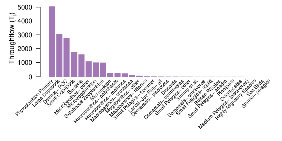
Figure 2: Rank order throughflow centrality for the Gulf of Main ecosystem.

Fig. 2 shows an example of rank ordered $T_{j}$ for the Gulf of Maine ecosystem network (Link et al., 2008). This shows the larger functional importance of phytoplankton, large and small copepods, detritus, bacteria in this system. This matches with the theoretical expectation that primary production and decomposition tend to be the critical components of ecosystem functioning (Wilkinson, 2006), but it also points to the importance of smaller consumers in the Gulf of Maine. Notice the similarity of this presentation to the rank–abundance and rank–productivity curves that Whittaker (1965) introduced to compare the relative importance of plants in a community. Like those original curves, $T_{j}$ suggests that in this system there are a few dominant or more important species and a long tail of functionally less critical species (e.g., Pinnipeds, Beleen whales, and pelagic sharks). The application section considers the generality of both of these patterns.

To facilitate comparisons between centrality measures, it is useful to consider the node throughflow scaled by the total system throughflow ($T_{j}/TST$) such that $\sum_{j=1}^{n}T_{j}/TST=1$. While the rank-ordering is preserved, rescaling in this way eliminates the units and differences in total magnitude between systems or other centrality measures. This focuses on intensive system differences while ignoring extensive differences present without the rescaling. Rescaling centrality measures is common, though it can introduce its own challenges (Ruhnau, 2000).

2.1.3 Path Decomposition

Path decomposition of throughflow lies at the core of ENA (Finn, 1976; Fath and Patten, 1999; Borrett et al., 2010), and shows why $T_{j}$ is a global measure of functional importance. It partitions the flow of energy–matter from the input (output) over paths of increasing length (number of directed edges, $m=0,1,2,\ldots,\infty$) within the system required to generate $T_{j}$. Recall that local centrality measures focus on the connections to a node’s nearest neighbors or a restricted neighborhood, while more global measures consider the relationships between all nodes within the system.

Path decomposition of flow starts by calculating the output oriented direct flow intensities $\mathbf{G}_{n\times n}=[g_{ij}]$ from node $j$ to $i$. These intensities are defined as

$$g_{ij} \equiv f_{ij}/T^{\textrm{out}}_{j}.$$ (3)

Here, $g_{ij}$ is the fraction of output throughflow at donor node $j$ contributed to node $i$. The $g_{ij}$ values are dimensionless and the column sums of $\mathbf{G}$ must lie between 0 and 1 with at least one column less than 1 because of thermodynamic constraints of the original model (Jørgensen et al., 1999).

The second step determines the output oriented integral flow intensities $\mathbf{N}=[n_{ij}]$ as

$$\mathbf{N} \equiv\sum_{m=0}^{\infty}\mathbf{G}^{m}$$ (4)

$$=\underbrace{\mathbf{I}}_{\textrm{Boundary}}+\underbrace{\mathbf{G}^{1}}_{\textrm{Direct}}+\underbrace{\mathbf{G}^{2}+\ldots+\mathbf{G}^{m}+\ldots}_{\textrm{Indirect}},$$ (5)

where $\mathbf{I_{n\times n}}=\mathbf{G}^{0}$ is the matrix multiplicative identity and the elements of $\mathbf{G}^{m}$ are the fractions of boundary flow that travel from node $j$ to $i$ over all pathways of length $m$. As the power series must converge given our initial model definition, the exact values of $\mathbf{N}$ can be found using the identity $\mathbf{N}=(\mathbf{I}-\mathbf{G})^{-1}$ . The $n_{ij}$ elements represent the intensity of boundary input that passes from $j$ to $i$ over all pathways of all lengths. These values integrate the boundary, direct, and indirect flows.

We can use $\mathbf{N}$ to recover $\mathbf{T}$ as follows:

$$\mathbf{T} =\mathbf{N}\mathbf{z}.$$ (6)

This suggests that the path decomposition of throughflow shown in equation (5) is a true partition of the pathway history of energy–matter in the system at steady-state.

The path decomposition in equation (5) shows how the throughflows are a global measure of centrality because the observed throughflows are generated by energy–matter moving over all pathways of all lengths such that the whole connected system is considered, not just a local neighborhood. Notice that the importance of longer pathways is naturally discounted as energy–matter is lost as it passes through nodes in the path. This discount or decay rate varies among ecosystems and model types (Borrett et al., 2010). Multiplication of the integral flow matrix by the boundary inputs to recover $T_{j}$ (equation 6) illustrates how the node throughflows capture the potential effect of heterogeneous boundary inputs known to be a factor in ecosystems (Borrett and Freeze, 2011).

2.2 Hubbell’s Status Score

Before Hannon (1973) applied Leontief’s (1965) economic input–output ideas to ecological systems, Hubbell (1965) applied the formalism to social systems. In doing so, he created a centrality measure that is known as Hubbell status or Hubbell centrality. Although Hubbell’s initial model was different than the ecological one presented in section 2.1.1, the analytical mathematics is parallel to that shown for throughflow analysis.

Hubbell (1965) started by modeling the interactions between individuals in a community using a weighted sociometric choice matrix $\mathbf{W}=[w_{ij}],(i,j=1,...,n)$, where $w_{ij}$ can be positive or negative and indicates individual $j$’s indication of the strength of relationship between him or herself and individual $i$. The integral relationship strength among the community members propagated across the whole set of pathways $\mathbf{R}$ are then determined as

$$\mathbf{R} =\mathbf{I}+\mathbf{W}^{1}+\mathbf{W}^{2}+\mathbf{W}^{3}+\ldots,$$ (7)

where $\mathbf{I}_{n\times n}$ is again the matrix multiplicative identity and $\mathbf{W}^{m}$ is the strength of relationship between any two community members over paths of length $m$. When the series converges, we can find $\mathbf{R}$ exactly as $\mathbf{R}=(\mathbf{I}-\mathbf{W})^{-1}$.

Building off of this analysis, Hubbell (1965) defined the status score $\mathbf{S}=[S_{i}]$ of member $i$ as

$$\mathbf{S} =\mathbf{R\times E}$$ (8)

where $\mathbf{E}_{n\times 1}=[e_{i}]$ are the system exogenous inputs.

While the initial model was different, the throughflow equation (6) is identical in form to Hubbell’s status shown in equation (8). Thus, what ecologists call throughflow $T_{j}$ is a special case of Hubbell’s status index $S_{i}$ when the model is defined as in section (2.1.1).

2.2.1 Eigenvector and Environ Centrality

To highlight its distinctiveness, $T_{j}$ is contrasted with two alternative global centrality measures: eigenvector centrality and environ centrality. As mentioned in the introduction, eigenvector centrality (EVC) describes the stable distribution of pathways, or when weighted as in flow networks the stable distribution of flow, passing through the nodes (Bonacich, 1972; Borgatti, 2005). In the context of directed flow networks, Fann and Borrett (2012) suggested using the average of the left $\mathbf{w}$ and right $\mathbf{v}$ hand eigenvector associated with the dominant eigenvalue of $\mathbf{G}$ to capture both the input and output, such that

$$EVC=[EVC_{i}]=\frac{(w_{i}+v_{i})}{2}.$$ (9)

Note, in this calculation $\mathbf{w}$ and $\mathbf{v}$ are assumed to have been normalized so that their sum equals 1, which also implies that $\sum_{i=1}^{n}EVC_{i}=1$. In symmetric networks like those for which the eigenvector centrality was first defined $v_{i}=w_{i}$ and averaging is not necessary. In directed flow networks $v_{i}\neq w_{i}$, and EVC captures the input and output oriented flows intensities.

Fann and Borrett (2012) introduced average environ centrality (AEC) and argued that it is a better centrality indicator for ecosystem flow networks in part because it captures both the equilibrium dynamics (like EVC) and transient dynamics that occur along the initial shorter pathways in equation (5). This is important because in highly dissipative systems like trophic ecosystems, a large fraction of the total transactions might occur in these shorter pathways. Specifically, Borrett et al. (2010) found that in nine trophic ecosystem models 95% of TST required at most paths of length nine. AEC is defined as

$$EC^{in} =[ec^{in}_{i}]=\frac{\sum_{j=1}^{n}n_{ij}}{\sum_{i=1}^{n}\sum_{j=1}^{n}n_{ij}}$$

$$EC^{out} =[ec^{out}_{j}]=\frac{\sum_{i=1}^{n}n_{ij}}{\sum_{i=1}^{n}\sum_{j=1}^{n}n_{ij}}$$

$$AEC =[aec_{k}]\frac{EC_{j}^{in}+EC_{j}^{out}}{2}.$$ (10)

Although AEC is an improvement on EVC, both measures still suffer from two problems. The first issue is that the calculations required for EVC and AEC are not intuitive, which could be a barrier to their wider use in ecology (Fawcett and Higginson, 2012). The second more substantive issue is that they fail to recognize or capture the external environmental forcing occurring in these open systems. Both measures are built on the non-dimensional flow intensity matrices that represent the potential flows or the flows if each node had a unit input. However, to recover the realized or observed system activity these matrices must be multiplied by the boundary vector as in equation 6 (see Hubbell, 1965). A critical issue is that the vector of boundary inputs in ecosystem models tends to be highly heterogeneous (Borrett and Freeze, 2011), which differentially excites the potential flow pathways captured in $\mathbf{G}$ and $\mathbf{N}$. Given these issues, in many applications $T_{j}$ is a better indicator of the functional importance of a node because its calculation is more intuitive and because it captures the system’s environmental forcing.

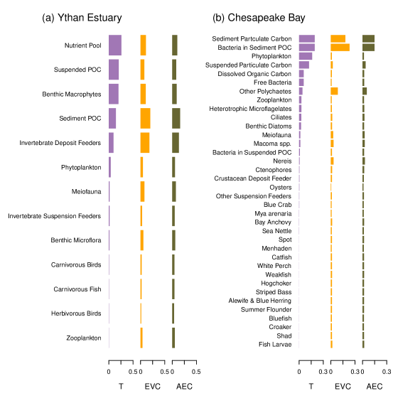
Figure 3: Comparison of throughflow centrality (TC), average eigenvector centrality (EVC), and average environ centrality (AEC) in the Ythan Estuary (a) and Chesapeake Bay (b) ecosystem networks. Model compartments are rank ordered by TC.

The difference between these indicators can be substantive as illustrated for the Ythan Estuary and Chesapeake Bay ecosystem models (Fig. 3). In the Ythan Estuary, $\mathbf{T}$ is highly rank correlated with EVC (Spearman’s $\rho=0.79$) and AEC ($\rho=0.82$), but $\mathbf{T}$ ranks the Nutrient Pool, Suspended POC, and Benthic Macrophytes as the top three nodes, which is not the case for the other two indicators. The first two of these nodes have boundary input. The Spearman rank correlation between $\mathbf{T}$ and EVC and AEC is generally less in the Chesapeake Bay model ($\rho=0.22$ and $\rho=0.55$, respectively). Again, EVC and AEC discount the importance of some nodes. In this case, the top three nodes – Phytoplankton, Suspended Particulate Carbon, and Dissolved Organic Carbon – have non-zero boundary input. Thus, $\mathbf{T}$ better captures the importance of nodes that connect the system to its external environment, and how this influence propagates throughout the system.

In summary, throughflow is a global centrality indicator of the functional importance of nodes in a flow network. It is a special case of what Hubbell (1965) defined as a status score in sociology. Due to the natural discounting of longer pathways as energy or matter dissipates from the system, it has the desirable properties of mesoscale centrality measures advocated for by Jordán et al. (2006). While it is similar to eigenvector and environ centrality measures, it is more intuitive to calculate and better captures the environmental forcing of the internal system activity. The next section applies $\mathbf{T}$ centrality to characterize the distribution of functional importance in 45 ecosystem models.

3 Application — Materials and Methods

Given that $T_{j}$ is a global indicator of an ecosystem component’s functional importance, we can now investigate the distribution of this importance in ecosystems.

3.1 Ecosystem Model Database

I applied flow analysis to 45 trophic ecosystem models selected from the literature and calculated $T_{j}$ to investigate the throughflow centrality distributions (Table 1). To be included in this data set, the models needed to have at least 10 compartments, have a food web at their core (i.e., trophic models), and be empirically-based in the sense that the original modelers were attempting to represent a real ecosystem and used empirical measurements to parametrize part of the fluxes. If two models existed in the literature for the same system, only the least aggregated model (higher $n$) was included. Ten (22%) of these models are included in Dr. Ulanowicz network collection on his website (http://www.cbl.umces.edu/~ulan/ntwk/network.html). This data set also overlaps 80% with the models recently analyzed for resource homogenization (Borrett and Salas, 2010), dominance of indirect effects (Salas and Borrett, 2011), and environ centrality (Fann and Borrett, 2012). The full set of models are available at http://people.uncw.edu/borretts/research.html. Forty-four percent of the models were not initially at steady-state, and were therefore balanced using the AVG2 algorithm (Allesina and Bondavalli, 2003).

3.2 Centrality Comparison

Rank correlation between $\mathbf{T}$ and AEC and EVC are shown for the Oyster Reef and Chesapeake Bay ecosystem models in section 2.2.1. Here, this result is generalized by examining distributions of the Spearman rank correlation between these measures in all 45 models in our database.

3.3 Thresholds, and Dominants

To characterize the $\mathbf{T}$ distributions within a model, I defined three thresholds. N₅₀ is the number of nodes required to cumulatively account for 50% of $TST$ when the compartments are rank ordered based on throughflow (largest to smallest). If a Monod function fit the cumulative flow distribution, N₅₀ would be equivalent to the half saturation constant. N₈₀ and N₉₅ are the number of nodes required to recover 80% and 95% of $TST$.

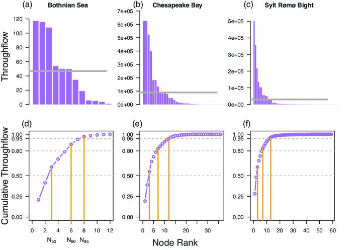
Figure 4: Rank ordered throughflow (a, b, c) and cumulative throughflow (d, e, f) for the Bothnian Sea (a,d), Chesapeake Bay (b,e), and Sylt-Rømø Bight network models (c,f). Throughflow has the units shown in Table 1. The thick horizontal line in a, b, and c shows what throughflow would be if each node contributed equally. The vertical lines in (c), (d), and (f) show the nodes at which 50% (N₅₀), 80% (N₈₀), and 95% (N₉₅) of the total system throughflow is achieved. For the Bothnian Sea, these thresholds are achieved at 3, 6, and 8, respectively. In the Chesapeake Bay they are 3, 6, and 12, while in the Sylt-Rømø Bight they are 3, 7, and 13.

These thresholds are illustrated for the Bothnian Sea, Chesapeake Bay, and Sylt-Rømø Bight ecosystems (Fig. 4). In the Bothnian Sea, only three nodes are required to generate 50% of the TST (N${}_{50}=3$), while 6 and 8 nodes are required to account for 80% and 95% of TST, respectively (N${}_{80}=6$ and N${}_{95}=8$). In the Chesapeake Bay model, these thresholds were N${}_{50}=3$, N${}_{80}=6$, and N${}_{95}=12$, and in the Sylt-Rømø Bight they were N${}_{50}=3$, N${}_{80}=7$, and N${}_{95}=13$.

As the three models shown here have different numbers of compartments, $n$, it is difficult to compare these thresholds directly. For better comparisons, I normalized the thresholds by the model size as N${}_{x}/n*100\%$. This gives the percent of nodes required to achieve the $x$% of $TST$. Fig. 4 shows that 33% of the model nodes are required to account for 95% of $TST$ in the Chesapeake Bay model while only 22% of the nodes were required in the Sylt-Rømø Bight model. This might be interpreted as indicating that system power is more concentrated in the Sylt-Rømø Bight model.

There are many ways of defining dominant species or compartments in ecological systems (e.g., Whittaker, 1965; Fann and Borrett, 2012). Here, dominant compartments in the ecosystem were defined as the smallest subset of nodes required to recover 50% of $TST$. This definition lets us investigate both how many nodes are required for this ($N_{50}$) as well as their identity. For analysis, these compartments were classified as primary producers (e.g., phytoplankton, submerged vegetation), dead organic matter (e.g., particulate organic matter, dissolved organic matter), bacteria (e.g., free living bacteria, bacteria, benthic bacteria), or other (e.g., filter feeders, meiofauna, large copepods). Detritus is technically a mixture of decomposers (some bacteria) with dead organic matter. For this analysis, detritus was grouped with the Dead Organic Matter.

4 Results

4.1 Centrality Comparison

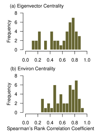
Figure 5: Histogram of Spearman rank correlation coefficients between throughflow centrality $T_{j}$ and (a) average eigenvector centrality (EVC) and (b) average environ centrality (AEC) in 45 ecosystem models.

As expected, EVC and AEC tend to be well correlated with $\mathbf{T}$ (Fig. 5). The median Spearman rank correlation between $\mathbf{T}$ and EVC is 0.69, with the values ranging between 0.11 and 0.87. Throughflow centrality is similarly correlated with AEC with a median value of 0.69. The distribution is visibly shifted to the right and has values ranging from 0.28 to 0.92. Notice that in no case is there 100% agreement or disagreement.

4.2 Thresholds

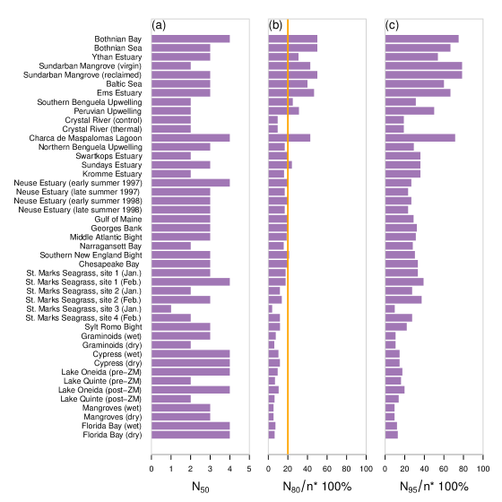
Figure 6: Rank order cumulative throughflow thresholds in 44 empirically based ecosystem models (models ordered by $n$ with smallest at the top): (a) number of nodes required to account for 50% (N₅₀), (b) percent of model nodes required to achieve 80% (N${}_{80}/n*100\%$), and (c) 95% (N${}_{95}/n*100\%$) of total system throughflow.

Figure 6 shows the cumulative flow development thresholds ($N_{50}$, $N_{80}/n$, $N_{95}/n$) for the 45 trophic network models. There are several trends to note. First, the maximum number of nodes necessary to account for 50% of $TST$ was 4. While in the Bothnian Bay ecosystem model this is 33% of the nodes, it is only 3.2% of the nodes in the Florida Bay model. Second, as the models increase in size ($n$) both $N_{80}/n$ and $N_{95}/n$ tend to decline. Third, Figure 6b shows that in the majority (73%) of the models, 20% of the nodes or fewer account for 80% or more of the system activity.

4.3 Dominants

Figure 6a shows that 4 or fewer nodes are required to account for 50% of the $TST$ and thus meet the criteria as dominants. The majority (46%) of the models analyzed had three dominant nodes, while another 29% had only two dominant compartments (Fig. 7a).

Table 2 identifies the 130 dominant nodes in each of the 45 ecosystems. The authors of the original models did not necessarily use identical categorizations for different ecosystem components, but it is possible to classify the compartments into four functional groups: primary producers, dead organic matter, bacteria, and a final category for anything else (other). Figure 7b shows the fraction of models that had at least one dominant in each of these categories. Thus, 82% of the models had at least one dominant compartment that functioned as a primary producer; 91% had a dominant compartment that was categorized as dead organic matter. Bacteria were also common. Only 9 of the dominant nodes did not fall into one of these three categories, and they only appeared in 7 of the models.

5 Discussion

Next I consider the theoretical development and its initial ecological application presented in this paper from three perspectives. First, I highlight some of the advantages and disadvantages of recognizing that system throughflow is a centrality indicator. Second, I contemplate the import of this discovery for understanding ecological system organization, growth, and development. Third, I identify additional possible applications of this innovation.

5.1 Throughflow as a Centrality

A primary contribution of this paper is to recognize that throughflow $\mathbf{T}$, a measure used by ecologists for some time (e.g., Finn, 1976; Ulanowicz, 1986; Fath and Patten, 1999), is a centrality measure as defined in the social science (Hubbell, 1965; Friedkin, 1991; Wasserman and Faust, 1994) and now used in general network science (Brandes and Erlebach, 2005). An advantage of connecting throughflow and centrality is that ecologists can now access, apply, and further develop the existing body of work on centrality. For example, many centrality measures have been proposed, but sociologists can generally classify them into one of three types (Freeman, 1979; Friedkin, 1991; Wasserman and Faust, 1994; Borgatti and Everett, 2006). The first type are degree based measures. These measures can vary in the size of the neighborhood considered – from the immediate local neighborhood to global measures that consider the whole system (e.g., Estrada, 2010). This type of centrality is generally interpreted as the influence of the node on the network activity or its power to change the activity (Bonacich, 1987). A second type of centrality is termed closeness and is based on the shortest paths or geodesic distances between nodes. Friedkin (1991) suggests that these measures indicate the immediacy of a node’s ability to influence the network. A third commonly described type of centrality is betweeness (Freeman, 1979; Freeman et al., 1991). A node’s betweeness centrality is its importance in transmitting activity between individuals or subgroups in the network. Thus, there is a recognition of several different but complementary ways in which individuals in a system can be central.

In this broader context of centralities, Hubbell’s status is a global, weighted, degree based centrality that is typically interpreted as the node’s influence on the whole system activity or its power to change the whole system activity (Borgatti, 2005; Brandes and Erlebach, 2005). The formulation allows the node’s centrality to be recursively changed by the centrality of the other nodes in the system as its walk connectivity is extended. Although Hubbell (1965) initially considered a potentially heterogeneous set of exogenous inputs, in practice a uniform set of inputs are typically used to consider the potential centrality. This is similar to the “unit” input analytical approach often used in network environ analysis (Fath and Patten, 1999; Whipple et al., 2007; Borrett and Freeze, 2011). In the ecological application of Hubbell centrality, the realized throughflow centrality is obtained using the observed exogenous inputs.

Ecologists can further benefit from the sociologists previous applications of centrality. For example, Hubbell initially used his centrality as a tool to detect subcommunities or cliques within the system. As this is again a common concern for ecologists (Pimm and Lawton, 1980; Allesina et al., 2005; Borrett et al., 2007), we may be able to utilize his procedure to address this problem in the future. This would follow Krause et al.’s (2003) successful application of a different social network analysis clique finding algorithm to food webs.

Another advantage is that we may be able to recognize other ENA measures as centrality type indicators. For example, several of Friedkin’s (1991) descriptions of alternative centrality measures for what he called “total effects centrality” were very similar to what Whipple et al. (2007) called total environ throughflow (TET). Thus, TET may also be a type of weighted degree centrality measure that indicates the relative contribution of each environ to the whole system activity. Hines et al. (2012) has already begun to explore this possibility while investigating nitrogen cycling model of the Cape Fear River estuary.

There are two potential disadvantages of recognizing throughflow as a centrality indicator. First, it could contribute to the proliferation of centrality measures that can be overwhelming. This has led to multiple papers trying to identify the unique contributions of specific indicators amongst a set of competing indicators (e.g., Newman, 2006; Jordán et al., 2007; Valente et al., 2008; Bauer et al., 2010; Baranyi et al., 2011). In this case, however, I argue that we are not creating a new centrality index to add to the confusion, but identifying that a commonly calculated measure is a form of an existing centrality measure. A second disadvantage might be that the current use and implementation of Hubbell’s centrality available in software packages may be simplified from its original formulation, as appears to be the case in Ucinet (Borgatti et al., 2002). The output of the Hubbell centrality analysis in Ucinet does not match the throughflow vector as calculated with NEA.m (Fath and Borrett, 2006)

As expected, $\mathbf{T}$ generally correlates well with average eigenvector centrality (EVC) and average environ centrality (AEC) for the 45 models examined. This suggests that these different global degree-based centrality measures capture some of the same information about the relative importance of the nodes for the system function. However, the correlations were variable – in some cases the rankings were quite different (e.g., median Spearman correlations were 0.69 and the lowest was 0.11) suggesting that each measure captured some unique information. Examining both the formulation of the three centrality measures as well as the example in Figure 3, a key difference is that $\mathbf{T}$ captures the importance of a node for connecting the system to the external world. For example in the Ythan estuary model, the Nutrient Pool and Suspended POC both have large inputs that contribute to their importance in $\mathbf{T}$. Thus in applications where the boundary inputs are an important consideration, an indicator like throughflow centrality may be the best choice. For example, Borrett and Freeze (2011) argued that this system–environment coupling is critical for ecologists and environmental scientists even when the analytical focus is on the within system environments.

5.2 Throughflow and Ecosystem Organization and Development

Ecologists have a long interest in the organization, growth, and development of ecosystems (e.g., Odum, 1969; Ulanowicz, 1986; Jørgensen et al., 2000; Gunderson and Holling, 2002; Loreau, 2010). What are the processes that create, constrain, and sustain ecological systems? Scientists investigating this problem have hypothesized a number of goal functions or orientors that might guide the growth and development of these self-organizing systems (Schneider and Kay, 1994; Müller and Leupelt, 1998; Jørgensen et al., 2007). Hypothesized orientors include the tendency for ecosystems to maximize power (Lotka, 1922; Odum and Pinkerton, 1955), maximize biomass or storage (Jørgensen and Mejer, 1979), maximize dissipation (Schneider and Kay, 1994), and maximize emergy (Odum, 1988). Fath et al. (2001) used the network framework to show how these different orientors can be complementary.

Patten (1995) suggested that throughflow in network models of energy flux can be interpreted as a measure of power in a thermodynamic sense. He argued that $TST$ indicates the total power output of an ecological system. This operationalized Lotka’s (1922) maximum power principle for evolutionary systems and Odum and Pinkerton’s (1955) hypothesis that ecological systems tend to maximize their power in a network context. Given this interpretation of $TST$, $T_{j}$ is therefore the partial power of each node ($j=1,2,\ldots,n$) in the network. Interestingly, this thermodynamic interpretation to throughflow aligns with the social interpretation of this type of centrality as the power to influence the system (Bonacich, 1987).

Recognizing that network nodes in ecosystem models represent subsystems in a hierarchical context (Allen and Star, 1982), then we can extend the maximum power hypothesis to each node. As all nodes would experience the same attraction to increase $T_{j}$, we might expect the $T_{j}$s to be more similar (towards a uniform distribution). However, this maximization remains restrained by the evolutionary constraints of the individual organisms, including their participation within the existing ecosystem (Walsh and Blows, 2009; Guimarães Jr et al., 2011). For example, Ulanowicz (1997, 2009) argues that the formation of autocatalytic cycles can be an agency for ecosystem growth and development. These cycles can provide the positive feedback and selective pressure for individual nodes to tend to increase their $T_{j}$. They also provide a selection pressure such that alternative nodes within an autocatalytic cycle compete for participation in throughflow and can be replaced by higher performing entities. Ulanowicz (1997) further argues that the tendency of these cycles for centripitality – in this context attracting and capturing more resources – leads to the emergence of a system autonomy from the material cause of the system. Thus, evolutionary constraints on species and the system constraints of interacting autocatalytic cycles might increase the variability of $T_{j}$ despite the homogenizing effect of the tendency to maximize throughflow.

The throughflow threshold analysis of the 45 ecosystem models presented here indicates that throughflow centrality is far from uniform as it appears to follow something more like Pareto’s 80-20 rule in which 80% of the activity is done by 20% of the group (Reed, 2001). This suggests that throughflow centrality may be similar to if not exactly the scale free degree distributions commonly found in other types of complex systems (Barabási, 2002). In addition, all but 8 of the dominant or most central nodes could be classified as primary producers, dead organic matter, or bacteria. This aligns with what we might expect from ecosystem theory in general and the importance of autocatalytic hypercycles like the autotroph $\leftrightarrow$ decomposer cycle (Ulanowicz, 1997; Wilkinson, 2006).

5.3 Applications

Network modeling and analysis, Input-Output Analysis, and material flow analysis have broad application. The ideas originated in macro economics (Leontief, 1966) and as has been discussed are used in both sociology and ecology. Thus, throughflow centrality may be useful in multiple domains of inquiry.

Beyond the theoretical considerations for ecosystem growth and development, there are a number of ways in which the throughflow centrality indicator could be usefully applied for ecosystem management, conservation, and restoration. For example, the throughflow centrality analysis suggests which species or groups of species should be targeted in the goal is to increase or decrease the system activity. The impact of manipulating a more central node should be greater than modifying a less central node.

Materials flow analysis is an important tool for industrial ecology (Bailey et al., 2004a, b; Suh and Kagawa, 2005; Gondkar et al., 2012) and urban metabolism (Kennedy et al., 2011; Zhang et al., 2012; Chen and Chen, 2012). The specific ENA methods described in this paper have been used to analyze the sustainability of urban metabolisms (Bodini and Bondavalli, 2002; Zhang et al., 2010; Chen and Chen, 2012). Chen and Chen (2012) shows how throughflow can be grouped according to compartment “trophic levels” to build productivity pyramids for cities that are then comparable to expected trophic productivity pyramids in ecology. Thus, the recognition that $\mathbf{T}$ is a centrality indicator could have a broad utility for these disciplines.

ENA is an ecoinformatic tool and shares many goals and characteristics with network analysis in the field of Systems Biology. For example, Hahn and Kern (2005) showed that genes with higher centrality tend to be functionally more important in protein-protein interaction networks. While thermodynamically conserved flows are not normally the focus of the systems biology network models (omics) making it difficult to apply the flow analysis and ENA more broadly, Kritz et al. (2010) suggest a way of liking a metabolic network model to the underlying chemical fluxes and reactions. If this technique proves robust, then the throughflow centrality might be useful in this domain as well.

6 Conclusions

In summary, this paper makes two primary contributions. First, I show that throughflow ($T_{j}$) in network input-output models is a global indicator of the relative importance or power of each node in the network with respect the whole system activity. As calculated in ecological network analysis, this is a special case of Hubbell centrality (Hubbell, 1965). Second, when applied to trophic network models of ecosystems, throughflow centrality shows the tendency of this power to be concentrated in a small set of nodes that tend to categorized as primary producers, dead organic material, or bacteria. This is consistent with previous theory regarding the growth and development of ecological systems.

To address the wicked problems (Rittel and Webber, 1973) of our time like economic challenges and global climate change, we will need to be both creative and innovative. An innovation in this paper is to join the throughflow concept in flow analysis and the centrality concept developed in the social sciences. I expect this to be a useful union that will enable new analysis and management of complex systems of many kinds including urban metabolisms, industrial ecosystems, and biogeochemical cycling and trophic dynamics in natural ecosystems.

7 Acknowledgments

Early ideas for this paper were first presented at the 2011 meeting of the International Society for Ecological Modelling in Beijing, China and benefited from conversations with several colleagues including Ursula Scharler, John Schramski, Bernie Patten, Sven Jørgensen, and Jeff Johnson. I also appreciate many colleagues sharing their network models with the Systems Ecology and Ecoinformatics Laboratory, including Dr. Baird, Link, Ulanowicz, and Sharler. Further, D.E. Hines provided comments on early manuscript drafts. This work was supported in part by UNCW and NSF (DEB-1020944).

Table 1: Forty-five empirically-based trophic ecosystem network models.

 

Model	units	$n^{\dagger}$	$C^{\dagger}$	$Boundary^{\dagger}$	$TST^{\dagger}$	$FCI^{\dagger}$	Source
Bothnian Bay	gC m-2 yr-1	12	0.22	44	184	0.23	Sandberg et al. (2000)
Bothnian Sea	gC m-2 yr-1	12	0.24	117	562	0.31	Sandberg et al. (2000)
Ythan Estuary	gC m-2 yr-1	13	0.23	1,259	4,182	0.24	Baird and Milne (1981)
Sundarban Mangrove (virgin)	kcal m-2 yr-1	14	0.22	117,959	441,214	0.16	Ray (2008)
Sundarban Mangrove (reclaimed)	kcal m-2 yr-1	14	0.22	38,485	103,057	0.05	Ray (2008)
Baltic Sea	mgC m-2 d-1	15	0.17	603	1,974	0.13	Baird et al. (1991)
Ems Estuary	mgC m-2 d-1	15	0.19	283	1,067	0.32	Baird et al. (1991)
Southern Benguela Upwelling	mgC m-2 d-1	16	0.23	715	2,546	0.31	Baird et al. (1991)
Peruvian Upwelling	mgC m-2 d-1	16	0.22	14,928	33,491	0.04	Baird et al. (1991)
Crystal River (control)	mgC m-2 d-1	21	0.19	7,358	15,063	0.07	Ulanowicz (1986)
Crystal River (thermal)	mgC m-2 d-1	21	0.14	6,018	12,032	0.09	Ulanowicz (1986)
Charca de Maspalomas Lagoon	mgC m-2 d-1	21	0.12	1,486,230	6,010,331	0.18	Almunia et al. (1999)
Northern Benguela Upwelling	mgC m-2 d-1	24	0.21	2,282	6,609	0.05	Heymans and Baird (2000)
Swartkops Estuary	mgC m-2 d-1	25	0.17	2,860	8,950	0.27	Scharler and Baird (2005)
Sundays Estuary	mgC m-2 d-1	25	0.16	4,442	11,940	0.22	Scharler and Baird (2005)
Kromme Estuary	mgC m-2 d-1	25	0.16	2,571	11,088	0.38	Scharler and Baird (2005)
Neuse Estuary (early summer 1997)	mgC m-2 d-1	30	0.09	4,385	13,828	0.12	Baird et al. (2004b)
Neuse Estuary (late summer 1997)	mgC m-2 d-1	30	0.11	4,640	13,036	0.13	Baird et al. (2004b)
Neuse Estuary (early summer 1998)	mgC m-2 d-1	30	0.09	4,569	14,025	0.12	Baird et al. (2004b)
Neuse Estuary (late summer 1998)	mgC m-2 d-1	30	0.1	5,641	15,032	0.11	Baird et al. (2004b)
Gulf of Maine	g ww m-2 yr-1	31	0.35	5,054	18,382	0.15	Link et al. (2008)
Georges Bank	g ww m-2 yr-1	31	0.35	4,381	16,890	0.18	Link et al. (2008)
Middle Atlantic Bight	g ww m-2 yr-1	32	0.37	4,869	17,917	0.18	Link et al. (2008)
Narragansett Bay	mgC m-2 yr-1	32	0.15	693,846	3,917,246	0.51	Monaco and Ulanowicz (1997)
Southern New England Bight	g ww m-2 yr-1	33	0.35	4,718	17,597	0.16	Link et al. (2008)
Chesapeake Bay	mgC m-2 yr-1	36	0.09	888,791	3,227,453	0.19	Baird and Ulanowicz (1989)
St. Marks Seagrass, site 1 (Jan.)	mgC m-2 d-1	51	0.08	515	1,316	0.13	Baird et al. (1998)
St. Marks Seagrass, site 1 (Feb.)	mgC m-2 d-1	51	0.08	602	1,591	0.11	Baird et al. (1998)
St. Marks Seagrass, site 2 (Jan.)	mgC m-2 d-1	51	0.07	603	1,383	0.09	Baird et al. (1998)
St. Marks Seagrass, site 2 (Feb.)	mgC m-2 d-1	51	0.08	801	1,921	0.08	Baird et al. (1998)
St. Marks Seagrass, site 3 (Jan.)	mgC m-2 d-1	51	0.05	7,809	12,651	0.01	Baird et al. (1998)
St. Marks Seagrass, site 4 (Feb.)	mgC m-2 d-1	51	0.08	1,433	2,865	0.04	Baird et al. (1998)
Sylt Rømø Bight	mgC m-2 d-1	59	0.08	683,448	1,781,029	0.09	Baird et al. (2004a)
Graminoids (wet)	gC m-2 yr-1	66	0.18	6,272	13,677	0.02	Ulanowicz et al. (2000)
Graminoids (dry)	gC m-2 yr-1	66	0.18	3,473	7,520	0.04	Ulanowicz et al. (2000)
Cypress (wet)	gC m-2 yr-1	68	0.12	1,419	2,572	0.04	Ulanowicz et al. (1997)
Cypress (dry)	gC m-2 yr-1	68	0.12	1,036	1,919	0.04	Ulanowicz et al. (1997)
Lake Oneida (pre-ZM)	gC m-2 yr-1	74	0.22	1,035	1,698	0.00	Miehls et al. (2009a)
Lake Quinte (pre-ZM)	gC m-2 yr-1	74	0.21	989	1,518	0.00	Miehls et al. (2009b)
Lake Oneida (post-ZM)	gC m-2 yr-1	76	0.22	811	1,463	0.00	Miehls et al. (2009a)
Lake Quinte (post-ZM)	gC m-2 yr-1	80	0.21	1,163	2,108	0.01	Miehls et al. (2009b)
Mangroves (wet)	gC m-2 yr-1	94	0.15	1,532	3,266	0.10	Ulanowicz et al. (1999)
Mangroves (dry)	gC m-2 yr-1	94	0.15	1,531	3,272	0.10	Ulanowicz et al. (1999)
Florida Bay (wet)	mgC m-2 yr-1	125	0.12	739	2,721	0.14	Ulanowicz et al. (1998)
Florida Bay (dry)	mgC m-2 yr-1	125	0.13	548	1,779	0.08	Ulanowicz et al. (1998)

  ^† $n$ is the number of nodes in the network model, $C=L/n^{2}$ is the model connectance when $L$ is the number of direct links or energy–matter transfers, $TST=\sum\sum{f_{ij}}+\sum{z_{i}}$ is the total system throughflow, and $FCI$ is the Finn Cycling Index (Finn, 1980).

Table 2: Dominant ecosystem components as identified by throughflow centrality with primary producers labeled with a green box, dead organic matter colored in a brown box with white letters, and bacteria in a pink box. These are the model nodes required to generate 50% of total system throughflow (N₅₀).

  Model $T_{1}$ $T_{2}$ $T_{3}$ $T_{4}$ Bothnian Bay DOM Bacteria Sediment C Pelagic Producers Bothnian Sea Macrofauna Sediment Carbon Pelagic Producers Ythan Estuary Nutrient Pool Suspended POC Benthic Macrophytes Sundarban Mangrove (virgin) Detritus Macrophytes Sundarban Mangrove (reclaimed) Detritus Macrophytes Benthic algae Baltic Sea Pelagic Production Mesozooplankton Suspended POC Ems Estuary Sediment POC Pelagic Producers Benthic Producers Southern Benguela Upwelling Suspended POC Phytoplankton Peruvian Upwelling Pelagic Producers Mesozooplankton Crystal River (control) Macrophytes Detritus Crystal River (thermal) Macrophytes Detritus Charca de Maspalomas Lagoon Sedimented POC Mesozooplankton Benthic Deposit Feeders Cyanobacteria Northern Benguela Upwelling POC DOC Bacteria Swartkops Estuary Sediment POC Sediment Bacteria Sundays Estuary Sediment POC Sediment Bacteria Phytoplankton Kromme Estuary Sediment POC Sediment Bacteria Neuse Estuary (early summer 1997) Free Living Bacteria DOC Sediment POC Sediment Bacteria Neuse Estuary (late summer 1997) DOC Free Living Bacteria Sediment POC Neuse Estuary (early summer 1998) Free Living Bacteria DOC Sediment POC Neuse Estuary (late summer 1998) DOC Free Living Bacteria Phytoplankton Gulf of Maine Phytoplankton-Primary Large Copepods Detritus–POC Georges Bank Phytoplankton-Primary Detritus–POC Bacteria Middle Atlantic Bight Phytoplankton-Primary Detritus–POC Bacteria Narragansett Bay Detritus Sediment POC Bacteria Southern New England Bight Phytoplankton-Primary Detritus–POC Bacteria Chesapeake Bay Sediment Particulate Carbon Bacteria in Sediment POC Phytoplankton St. Marks Seagrass, site 1 (Jan.) Benthic Bacteria Micro-epiphytes Sediment POC St. Marks Seagrass, site 1 (Feb.) Benthic Bacteria Sediment POC Benthic algae Meiofauna St. Marks Seagrass, site 2 (Jan.) Micro-epiphytes Sediment POC St. Marks Seagrass, site 2 (Feb.) Sediment POC Benthic algae Benthic Bacteria St. Marks Seagrass, site 3 (Jan.) Micro-epiphytes St. Marks Seagrass, site 4 (Feb.) Pinfish Sediment POC Sylt-Rømø Bight Sediment POC Microphytobenthos Phytoplankton Everglade Graminoids (wet) Sediment Carbon Periphyton Refractory Detritus Everglade Graminoids (dry) Periphyton Sediment Carbon Cypress (wet) Refractory Detritus Cypress Living Sediment Liable Detritus Cypress (dry) Refractory Detritus Living sediment Understory Liable Detritus Lake Oneida (pre-ZM) Pelagic Detritus Diatoms Blue-myGreen Algae Epiphytes Lake Quinte (pre-ZM) Pelagic Detritus Diatoms Lake Oneida (post-ZM) Diatoms Epiphytes Pelagic Detritus Blue-myGreen Algae Lake Quinte (post-ZM) Zebra Mussels Diatoms Mangroves (wet) Carbon in Sediment Leaf Other Primary Producers Mangroves (dry) Carbon in Sediment Leaf Other Primary Producers Florida Bay (wet) Benthic POC Water POC Water Flagellates Thalassia Florida Bay (dry) Benthic POC Water POC Thalassia DOC  

Figure 7: Dominant analysis: (a) the frequency of the 45 models with 1, 2, 3, or 4 dominant nodes ($N_{50}$), and (b) the percent of models with at least one dominant node in the three functional categories.

References

- Allen and Star (1982) Allen, T. F. H., Star, T. B., 1982. Hierarchy: Perspectives for Ecological Complexity. University of Chicago Press.
- Allesina et al. (2005) Allesina, S., Bodini, A., Bondavalli, C., 2005. Ecological subsystems via graph theory: the role of strongly connected components. Oikos 110, 164–176.
- Allesina and Bondavalli (2003) Allesina, S., Bondavalli, C., 2003. Steady state of ecosystem flow networks: A comparison between balancing procedures. Ecol. Model. 165, 221–229.
- Allesina and Pascual (2009) Allesina, S., Pascual, M., 2009. Googling food webs: can an eigenvector measure species’ importance for coextinctions? PLoS Comp. Bio. 5, 1175–1177.
- Almunia et al. (1999) Almunia, J., Basterretxea, G., Aistegui, J., Ulanowicz, R. E., 1999. Benthic–pelagic switching in a coastal subtropical lagoon. Estuar. Coast. Shelf Sci. 49, 221–232.
- Bailey et al. (2004a) Bailey, R., Allen, J., Bras, B., 2004a. Applying ecological input-output flow analysis to material flows in industrial systems: Part I: Tracing flows. J. Ind. Ecol. 8 (1-2), 45–68.
- Bailey et al. (2004b) Bailey, R., Bras, B., Allen, J., 2004b. Applying ecological input-output flow analysis to material flows in industrial systems: Part II: Flow metrics. J. Ind. Ecol. 8 (1-2), 69–91.
- Baird et al. (2004a) Baird, D., Asmus, H., Asmus, R., 2004a. Energy flow of a boreal intertidal ecosystem, the Sylt-Rømø Bight. Mar. Ecol. Prog. Ser. 279, 45–61.
- Baird et al. (2004b) Baird, D., Christian, R. R., Peterson, C. H., Johnson, G. A., 2004b. Consequences of hypoxia on estuarine ecosystem function: Energy diversion from consumers to microbes. Ecol. Appl. 14, 805–822.
- Baird et al. (1998) Baird, D., Luczkovich, J., Christian, R. R., 1998. Assessment of spatial and temporal variability in ecosystem attributes of the St Marks National Wildlife Refuge, Apalachee Bay, Florida. Estuar. Coast. Shelf Sci. 47, 329–349.
- Baird et al. (1991) Baird, D., McGlade, J. M., Ulanowicz, R. E., 1991. The comparative ecology of six marine ecosystems. Philos. Trans. R. Soc. Lond. B 333, 15–29.
- Baird and Milne (1981) Baird, D., Milne, H., 1981. Energy flow in the Ythan Estuary, Aberdeenshire, Scotland. Estuar. Coast. Shelf Sci. 13, 455–472.
- Baird and Ulanowicz (1989) Baird, D., Ulanowicz, R. E., 1989. The seasonal dynamics of the Chesapeake Bay ecosystem. Ecol. Monogr. 59, 329–364.
- Barabási (2002) Barabási, A. L., 2002. Linked: the new science of networks. Perseus, Cambridge, Mass.
- Baranyi et al. (2011) Baranyi, G., Saura, S., Podani, J., Jordán, F., 2011. Contribution of habitat patches to network connectivity: Redundancy and uniqueness of topological indices. Ecol. Indic. 11 (5), 1301–1310.
- Bauer et al. (2010) Bauer, B., Jord’an, F., Podani, J., 2010. Node centrality indices in food webs: Rank orders versus distributions. Ecol. Comp. 7, 471–477.
- Bodin and Saura (2010) Bodin, O., Saura, S., 2010. Ranking individual habitat patches as connectivity providers: Integrating network analysis and patch removal experiments. Ecol. Model. 221, 2393–2405.
- Bodini and Bondavalli (2002) Bodini, A., Bondavalli, C., 2002. Towards a sustainable use of water resources: a whole-ecosystem approach using network analysis. Int. J. Environ. Pol. 18, 463–485.
- Bonacich (1972) Bonacich, P., 1972. Factoring and weighting approaches to clique identification. J. Math. Soc. 2, 113–120.
- Bonacich (1987) Bonacich, P., 1987. Power and centrality: A family of measures. Am. J. Sociol. 92 (5), 1170–1182.
- Borgatti et al. (2002) Borgatti, S., Everett, M., Freeman, L., 2002. Ucinet for Windows: Software for Social Network Analysis. Analytic Technologies, Harvard, MA.
- Borgatti (2005) Borgatti, S. P., 2005. Centrality and network flow. Soc. Networks 27, 55–71.
- Borgatti and Everett (2006) Borgatti, S. P., Everett, M. G., 2006. A graph-theoretic perspective on centrality. Soc. Networks 28, 466–484.
- Borrett et al. (2007) Borrett, S. R., Fath, B. D., Patten, B. C., 2007. Functional integration of ecological networks through pathway proliferation. J. Theor. Biol. 245, 98–111.
- Borrett and Freeze (2011) Borrett, S. R., Freeze, M. A., 2011. Reconnecting environs to their environment. Ecol. Model. 222, 2393–2403.
- Borrett and Salas (2010) Borrett, S. R., Salas, A. K., 2010. Evidence for resource homogenization in 50 trophic ecosystem networks. Ecol. Model. 221, 1710–1716.
- Borrett et al. (2010) Borrett, S. R., Whipple, S. J., Patten, B. C., 2010. Rapid development of indirect effects in ecological networks. Oikos 119, 1136–1148.
- Brandes and Erlebach (2005) Brandes, U., Erlebach, T. (Eds.), 2005. Network Analysis: Methodological Foundations. Springer-Verlag, Berlin, Heidelberg.
- Chen and Chen (2012) Chen, S., Chen, B., 2012. Network environ perspective for urban metabolism and carbon emissions: A case study of Vienna, Austria. Environ. Sci. Tech. 46 (8), 4498–4506.
- Dayton (1972) Dayton, P. K., 1972. Toward an understanding of community resilience and the potential effects of enrichments to the benthos at McMurdo Sound, Antarctica. In: Parker, E. (Ed.), Proceedings of the colloquium on conservation problems in Antarctica. Allen Press, Lawrence, KS.
- Ellison et al. (2005) Ellison, A., Bank, M., Clinton, B., Colburn, E., Elliott, K., Ford, C., Foster, D., Kloeppel, B., Knoepp, J., Lovett, G., et al., 2005. Loss of foundation species: consequences for the structure and dynamics of forested ecosystems. Front. Ecol. Environ. 3 (9), 479–486.
- Estrada (2010) Estrada, E., 2010. Generalized walks-based centrality measures for complex biological networks. J. Theor. Biol. 263, 556 – 565.
- Estrada and Bodin (2008) Estrada, E., Bodin, O., 2008. Using network centrality measures to manage landscape connectivity. Ecol. Appl. 18 (7), 1810–1825.
- Fann and Borrett (2012) Fann, S. L., Borrett, S. R., 2012. Environ centrality reveals the tendency of indirect effects to homogenize the functional importance of species in ecosystems. J. Theor. Biol. 294, 74–86.
- Fath and Borrett (2006) Fath, B. D., Borrett, S. R., 2006. A Matlab© function for network environ analysis. Environ. Model. Softw. 21, 375–405.
- Fath and Patten (1999) Fath, B. D., Patten, B. C., 1999. Review of the foundations of network environ analysis. Ecosystems 2, 167–179.
- Fath et al. (2001) Fath, B. D., Patten, B. C., Choi, J. S., 2001. Complementarity of ecological goal functions. J. Theor. Biol. 208, 493–506.
- Fath et al. (2007) Fath, B. D., Scharler, U. M., Ulanowicz, R. E., Hannon, B., 2007. Ecological network analysis: network construction. Ecol. Model. 208, 49–55.
- Fawcett and Higginson (2012) Fawcett, T., Higginson, A., 2012. Heavy use of equations impedes communication among biologists. Proc. Nat. Acad. Sci. 109 (29), 11735–11739.
- Finn (1976) Finn, J. T., 1976. Measures of ecosystem structure and function derived from analysis of flows. J. Theor. Biol. 56, 363–380.
- Finn (1980) Finn, J. T., 1980. Flow analysis of models of the Hubbard Brook ecosystem. Ecology 61, 562–571.
- Freeman et al. (1991) Freeman, L., Borgatti, S., White, D., 1991. Centrality in valued graphs: A measure of betweenness based on network flow. Soc. Networks 13 (2), 141–154.
- Freeman (1979) Freeman, L. C., 1979. Centrality in networks. I. Conceptual clarification. Soc. Networks 1, 215–239.
- Friedkin (1991) Friedkin, N., 1991. Theoretical foundations for centrality measures. Am. J. Sociol. 96, 1478–1504.
- Gondkar et al. (2012) Gondkar, S., Sriramagiri, S., Zondervan, E., 2012. Methodology for assessment and optimization of industrial eco-systems. Challenges 3 (1), 49–69.
- Guimarães Jr et al. (2011) Guimarães Jr, P., Jordano, P., Thompson, J., 2011. Evolution and coevolution in mutualistic networks. Ecol. Lett. 14, 877––885.
- Gunderson and Holling (2002) Gunderson, L. H., Holling, C. S., 2002. Panarchy: Understanding transformations in human and natural systems. Island Press, Washington, DC.
- Hahn and Kern (2005) Hahn, M., Kern, A., 2005. Comparative genomics of centrality and essentiality in three eukaryotic protein-interaction networks. Mol. Biol. Evol. 22 (4), 803–806.
- Hannon (1973) Hannon, B., 1973. The structure of ecosystems. J. Theor. Biol. 41, 535–546.
- Heymans and Baird (2000) Heymans, J. J., Baird, D., 2000. A carbon flow model and network analysis of the northern Benguela upwelling system, Namibia. Ecol. Model. 126, 9–32.
- Hines et al. (2012) Hines, D., Lisa, J., Song, B., Tobias, C., Borrett, S., 2012. A network model shows the importance of coupled processes in the microbial N cycle in the Cape Fear River estuary. Estuar. Coast. Shelf Sci. 106, 45–57.
- Hooper et al. (2005) Hooper, D., Chapin Iii, F., Ewel, J., Hector, A., Inchausti, P., Lavorel, S., Lawton, J., Lodge, D., Loreau, M., Naeem, S., et al., 2005. Effects of biodiversity on ecosystem functioning: a consensus of current knowledge. Ecol. Monogr. 75 (1), 3–35.
- Hubbell (1965) Hubbell, C. H., 1965. An input-output approach to clique identification. Sociometry, 377–399.
- Ibarra (1993) Ibarra, H., 1993. Network centrality, power, and innovation involvement: Determinants of technical and administrative roles. Acad. Manage. J. 36, 471–501.
- Jones et al. (1994) Jones, C. G., Lawton, J. H., Shachak, M., 1994. Organisms as ecosystem engineers. Oikos, 373–386.
- Jordán et al. (2003) Jordán, F., Baldi, A., Orci, K. M., Racz, I., Varga, Z., 2003. Characterizing the importance of habitat patches and corridors in maintaining the landscape connectivity of a pholidoptera transsylvanica (orthoptera) metapopulation. Landscape Ecol. 18, 83–92.
- Jordán et al. (2007) Jordán, F., Benedek, Z., Podani, J., 2007. Quantifying positional importance in food webs: a comparison of centrality indices. Ecol. Model. 205, 270–275.
- Jordán et al. (2006) Jordán, F., Liu, W., Davis, A., 2006. Topological keystone species: measures of positional importance in food webs. Oikos 112 (3), 535–546.
- Jørgensen et al. (2007) Jørgensen, S. E., Fath, B. D., Bastianoni, S., Marques, J. C., Müller, F., Nielsen, S., Patten, B. C., Tiezzi, E., Ulanowicz, R. E., 2007. A new ecology: Systems perspective. Elsevier, Amsterdam.
- Jørgensen and Mejer (1979) Jørgensen, S. E., Mejer, H. F., 1979. A holistic approach to ecological modelling. Ecol. Model. 7, 169–189.
- Jørgensen et al. (1999) Jørgensen, S. E., Patten, B. C., Straškraba, M., 1999. Ecosystems emerging: 3. openness. Ecol. Model. 117, 41–64.
- Jørgensen et al. (2000) Jørgensen, S. E., Patten, B. C., Straškraba, M., 2000. Ecosystems emerging: 4. growth. Ecol. Model. 126, 249–284.
- Kennedy et al. (2011) Kennedy, C., Pincetl, S., Bunje, P., 2011. The study of urban metabolism and its applications to urban planning and design. Environ. Pol. 159 (8), 1965–1973.
- Koschützki et al. (2005) Koschützki, D., Lehmann, K. A., Peeters, L., Richter, S., Tenfelde-Podehl, D., Zlotowski, O., 2005. Centrality indices. In: Brandes, U., Erlebach, T. (Eds.), Network Analysis: Methodological Foundations. Springer-Verlag, Berlin, Heidelberg, pp. 16–61.
- Krause et al. (2003) Krause, A. E., Frank, K. A., Mason, D. M., Ulanowicz, R. E., Taylor, W. W., 2003. Compartments revealed in food-web structure. Nature 426, 282–285.
- Kritz et al. (2010) Kritz, M., Trindade dos Santos, M., Urrutia, S., Schwartz, J., 2010. Organising metabolic networks: Cycles in flux distributions. J. Theor. Biol. 265 (3), 250–260.
- Lawton (1994) Lawton, J. H., 1994. What do species do in ecosystems? Oikos 71, 367–374.
- Leontief (1965) Leontief, W. W., 1965. The structure of the American economy. Sci. Am. 212, 25–35.
- Leontief (1966) Leontief, W. W., 1966. Input–Output Economics. Oxford University Press, New York.
- Lindeman (1942) Lindeman, R. L., 1942. The trophic-dynamic aspect of ecology. Ecology 23, 399–418.
- Link et al. (2008) Link, J., Overholtz, W., O’Reilly, J., Green, J., Dow, D., Palka, D., Legault, C., Vitaliano, J., Guida, V., Fogarty, M., Brodziak, J., Methratta, L., Stockhausen, W., Col, L., Griswold, C., 2008. The northeast US continental shelf energy modeling and analysis exercise (EMAX): Ecological network model development and basic ecosystem metrics. J. Mar. Syst. 74, 453–474.
- Loreau (2010) Loreau, M., 2010. From populations to ecosystems: Theoretical foundations for a new ecological synthesis. Princeton University Press, Princeton, NJ.
- Lotka (1922) Lotka, A. J., 1922. Contribution to the energetics of evolution. Proc. Nat. Acad. Sci. USA 8, 147–151.
- Martín González et al. (2010) Martín González, A., Dalsgaard, B., Olesen, J., 2010. Centrality measures and the importance of generalist species in pollination networks. Ecol. Comp. 7 (1), 36–43.
- Miehls et al. (2009a) Miehls, A. L. J., Mason, D. M., Frank, K. A., Krause, A. E., Peacor, S. D., Taylor, W. W., 2009a. Invasive species impacts on ecosystem structure and function: A comparison of Oneida Lake, New York, USA, before and after zebra mussel invasion. Ecol. Model. 220 (22), 3194–3209.
- Miehls et al. (2009b) Miehls, A. L. J., Mason, D. M., Frank, K. A., Krause, A. E., Peacor, S. D., Taylor, W. W., 2009b. Invasive species impacts on ecosystem structure and function: A comparison of the Bay of Quinte, Canada, and Oneida Lake, USA, before and after zebra mussel invasion. Ecol. Model. 220, 3182–3193.
- Mills et al. (1993) Mills, L., Soule, M., Doak, D., 1993. The keystone-species concept in ecology and conservation. BioScience 43 (4), 219–224.
- Monaco and Ulanowicz (1997) Monaco, M. E., Ulanowicz, R. E., 1997. Comparative ecosystem trophic structure of three us mid-Atlantic estuaries. Mar. Ecol. Prog. Ser. 161, 239–254.
- Müller and Leupelt (1998) Müller, F., Leupelt, M., 1998. Eco targets, goal functions, and orientors. Springer, New York.
- Newman (2006) Newman, M. E. J., 2006. Finding community structure in networks using the eigenvectors of matricies. Phys. Rev. E 74, –036104.
- Odum (1959) Odum, E. P., 1959. Fundamentals of Ecology, second edition. W.B. Saunders Company, Philadelphia.
- Odum (1969) Odum, E. P., 1969. The strategy of ecosystem development. Science 164, 262–270.
- Odum (1988) Odum, H., 1988. Self-organization, transformity, and information. Science 242 (4882), 1132–1139.
- Odum and Pinkerton (1955) Odum, H., Pinkerton, R., 1955. Time’s speed regulator: the optimum efficiency for maximum power output in physical and biological systems. Amer. Sci. 43 (2), 331–343.
- Paine (1966) Paine, R. T., 1966. Food web complexity and species diversity. Am. Nat. 100, 65–75.
- Patten (1995) Patten, B. C., 1995. Network integration of ecological extremal principles: Exergy, emergy, power, ascendency, and indirect effects. Ecol. Model. 79, 75–84.
- Patten et al. (1976) Patten, B. C., Bosserman, R. W., Finn, J. T., Cale, W. G., 1976. Propagation of cause in ecosystems. In: Patten, B. C. (Ed.), Systems Analysis and Simulation in Ecology, Vol. IV. Academic Press, New York, pp. 457–579.
- Pimm and Lawton (1980) Pimm, S., Lawton, J., 1980. Are food webs divided into compartments? The J. Anim. Ecol., 879–898.
- Power et al. (1996) Power, M. E., Tilman, D., Estes, J. A., Menge, B. A., Bond, W. J., Mills, L. S., Daily, G., Castilla, J. C., Lubchenco, J., Paine, R. T., 1996. Challenges in the quest for keystones. Bioscience 46 (8), 609–620.
- Ray (2008) Ray, S., 2008. Comparative study of virgin and reclaimed islands of Sundarban mangrove ecosystem through network analysis. Ecol. Model. 215, 207–216.
- Reed (2001) Reed, W., 2001. The Pareto, Zipf and other power laws. Econ. Lett. 74 (1), 15–19.
- Rittel and Webber (1973) Rittel, H., Webber, M., 1973. Dilemmas in a general theory of planning. Policy sci. 4 (2), 155–169.
- Ruhnau (2000) Ruhnau, B., 2000. Eigenvector-centrality — node-centrality? Soc. Networks 22 (4), 357–365.
- Saavedra et al. (2011) Saavedra, S., Stouffer, D., Uzzi, B., Bascompte, J., 2011. Strong contributors to network persistence are the most vulnerable to extinction. Nature 478, 233–235.
- Salas and Borrett (2011) Salas, A. K., Borrett, S. R., 2011. Evidence for dominance of indirect effects in 50 trophic ecosystem networks. Ecol. Model. 222, 1192–1204.
- Sandberg et al. (2000) Sandberg, J., Elmgren, R., Wulff, F., 2000. Carbon flows in Baltic Sea food webs — a re-evaluation using a mass balance approach. J. Mar. Syst. 25, 249–260.
- Sazima et al. (2010) Sazima, C., Guimaraes, Jr., P. R., dos Reis, S. F., Sazima, I., 2010. What makes a species central in a cleaning mutualism network? Oikos 119 (8), 1319–1325.
- Scharler and Baird (2005) Scharler, U. M., Baird, D., 2005. A comparison of selected ecosystem attributes of three South African estuaries with different freshwater inflow regimes, using network analysis. J. Mar. Syst. 56, 283–308.
- Schneider and Kay (1994) Schneider, E. D., Kay, J. J., 1994. Life as a manifestation of the second law of thermodynamics. Math. Comput. Model. 19, 25–48.
- Schramski et al. (2011) Schramski, J. R., Kazanci, C., Tollner, E. W., 2011. Network environ theory, simulation and EcoNet© 2.0. Environ. Model. Softw. 26, 419–428.
- Scotti et al. (2007) Scotti, M., Podani, J., Jordán, F., 2007. Weighting, scale dependence and indirect effects in ecological networks: a comparative study. Ecol. Comp. 4, 148–159.
- Suh and Kagawa (2005) Suh, S., Kagawa, S., 2005. Industrial ecology and input-output economics: an introduction. Econ. Sys. Res. 17 (4), 349–364.
- Ulanowicz (1986) Ulanowicz, R. E., 1986. Growth and development: ecosystems phenomenology. Springer–Verlag, New York.
- Ulanowicz (1997) Ulanowicz, R. E., 1997. Ecology, the ascendent perspective. Columbia University Press, New York.
- Ulanowicz (2009) Ulanowicz, R. E., 2009. Autocatalysis. In: Jørgensen, S. E., Fath, B. D. (Eds.), Systems Ecology. Vol 1 of Encyclopedia of Ecology. Vol. 1. Elsevier, Oxford, pp. 288–290.
- Ulanowicz et al. (1997) Ulanowicz, R. E., Bondavalli, C., Egnotovich, M. S., 1997. Network analysis of trophic dynamics in South Florida ecosystem, fy 96: The cypress wetland ecosystem. Annual Report to the United States Geological Service Biological Resources Division Ref. No. [UMCES]CBL 97-075, Chesapeake Biological Laboratory, University of Maryland.
- Ulanowicz et al. (1998) Ulanowicz, R. E., Bondavalli, C., Egnotovich, M. S., 1998. Network analysis of trophic dynamics in South Florida ecosystem, fy 97: The Florida bay ecosystem. Annual Report to the United States Geological Service Biological Resources Division Ref. No. [UMCES]CBL 98-123, Chesapeake Biological Laboratory, University of Maryland.
- Ulanowicz et al. (1999) Ulanowicz, R. E., Bondavalli, C., Heymans, J. J., Egnotovich, M. S., 1999. Network analysis of trophic dynamics in South Florida ecosystem, fy 98: The mangrove ecosystem. Annual Report to the United States Geological Service Biological Resources Division Ref. No.[UMCES] CBL 99-0073; Technical Report Series No. TS-191-99, Chesapeake Biological Laboratory, University of Maryland.
- Ulanowicz et al. (2000) Ulanowicz, R. E., Bondavalli, C., Heymans, J. J., Egnotovich, M. S., 2000. Network analysis of trophic dynamics in South Florida ecosystem, fy 99: The graminoid ecosystem. Annual Report to the United States Geological Service Biological Resources Division Ref. No. [UMCES] CBL 00-0176, Chesapeake Biological Laboratory, University of Maryland.
- Ulanowicz and Puccia (1990) Ulanowicz, R. E., Puccia, C. J., 1990. Mixed trophic impacts in ecosystems. Coenoses 5, 7–16.
- Valente et al. (2008) Valente, T. W., Coronges, K., Lakon, C., Costenbader, E., 2008. How correlated are network centrality measures? Connections 22 (1), 16–26.
- Walker (1992) Walker, B., 1992. Biodiversity and ecological redundancy. Conserve. Biol. 6 (1), 18–23.
- Walsh and Blows (2009) Walsh, B., Blows, M. W., 2009. Abundant genetic variation plus strong selection = multivariate genetic constraints: A geometric view of adaptation. Annu. Rev. Ecol. Evol. S. 40, 41–59.
- Wasserman and Faust (1994) Wasserman, S., Faust, K., 1994. Social network analysis: methods and applications. Cambridge University Press, Cambridge; New York.
- Whipple et al. (2007) Whipple, S. J., Borrett, S. R., Patten, B. C., Gattie, D. K., Schramski, J. R., Bata, S. A., 2007. Indirect effects and distributed control in ecosystems: Comparative network environ analysis of a seven-compartment model of nitrogen flow in the Neuse River Estuary, USA—time series analysis. Ecol. Model. 206, 1–17.
- Whittaker (1965) Whittaker, R. H., 1965. Dominance and Diversity in Land Plant Communities: Numerical relations of species express the importance of competition in community function and evolution. Science 147 (3655), 250–260.
- Wilkinson (2006) Wilkinson, D. M., 2006. Fundamental processes in ecology: an Earth systems approach. Oxford University Press, Oxford.
- Zhang et al. (2012) Zhang, Y., Liu, H., Li, Y., Yang, Z., Li, S., Yang, N., 2012. Ecological network analysis of China’s societal metabolism. J. Environ. Manage. 93 (1), 254–263.
- Zhang et al. (2010) Zhang, Y., Yang, Z., Fath, B., 2010. Ecological network analysis of an urban water metabolic system: Model development, and a case study for Beijing. Sci. Total Env. 408, 4702–4711.