Stabilizability and Norm-Optimal Control Design subject to Sparsity Constraints

Abstract

Consider that a linear time-invariant (LTI) plant is given and that we wish to design a stabilizing controller for it. Admissible controllers are LTI and must comply with a pre-selected sparsity pattern. The sparsity pattern is assumed to be quadratically invariant (QI) with respect to the plant, which, from prior results, guarantees that there is a convex parametrization of all admissible stabilizing controllers provided that an initial admissible stable stabilizing controller is provided. This paper addresses the previously unsolved problem of determining necessary and sufficient conditions for the existence of an admissible stabilizing controller. The main idea is to cast the existence of such a controller as the feasibility of an exact model-matching problem with stability restrictions, which can be tackled using existing methods. Furthermore, we show that, when it exists, the solution of the model-matching problem can be used to compute an admissible stabilizing controller. This method also leads to a convex parametrization that may be viewed as an extension of Youla’s classical approach so as to incorporate sparsity constraints. Applications of this parametrization on the design of norm-optimal controllers via convex methods are also explored. An illustrative example is provided, and a special case is discussed for which the exact model matching problem has a unique and easily computable solution.

I Introduction

In this paper, we deal with the problem of output–feedback stabilization for linear time–invariant (LTI) plants using sparsity-constrained LTI controllers. The sparsity constraints are specified by a binary matrix with the same number of rows and columns as the controller. More specifically, entries of the controller must be zero whenever the corresponding element of the constraint matrix is zero, and are unrestricted otherwise.

I-A Previous Results

The convex parametrization [2] proposed by Youla, which spans all LTI controllers that stabilize a prescribed LTI plant, popularized the so–called factorization approach [3] to the analysis and synthesis of LTI feedback systems. The methods proposed in [4] cast the search space in a ring, which provides additional insight and tools rooted on algebraic methods. However useful in expressing the design of norm-optimal controllers as convex programs, Youla’s parametrization does not allow for sparsity constraints on the controller. The recent work in [5, 6, 7, 8] partially bridges this gap by identifying properties that the sparsity pattern of the plant and the one imposed on the controller must satisfy so that a convex parametrization of all stabilizing controllers may exist. These recently discovered methods spring from invariance principles that are valid in the presence of what the authors define as funnel causality, and their validity extended to the more general class [9] of quadratically invariant sparsity patterns [10, 11]. The invariance condition in [10, 11] can be readily checked via an algebraic test, which, if true, assures that if there exists a stable stabilizing controller that satisfies the sparsity constraint then the set of all sparsity-constrained stabilizing controllers admits a convex parametrization based on a modification of the one in [12]. Subsequent work [13] has provided another convex parametrization that is guaranteed to exist under quadratic invariance, provided that a stabilizing controller that satisfies the sparsity constraint is given, and unlike prior work is not required to be itself stable. It has also been shown recently [14] that quadratic invariance of the set of controllers is necessary for the existence of the convex parametrization proposed in [10, 11].

I-B Contributions of this paper:

The main results of this paper are motivated by the following problem.

Problem I.1.

Consider that an LTI plant and a commensurate quadratically invariant sparsity constraint are given. Is the plant stabilizable by an LTI controller that satisfies the sparsity constraint? If one exists then compute it and give a convex parametrization of all stabilizing sparsity-constrained controllers.

For a given plant, in this paper we establish necessary and sufficient conditions for the existence of a stabilizing LTI controller, subject to pre-specified quadratically invariant sparsity constraints. If one exists then our analysis also provides a method to construct a stabilizing controller that respects the sparsity constraints. Since all existing convex parametrizations presuppose prior knowledge of a stabilizing sparsity constrained controller [10], our results bridge an important gap in the design process.

In our solution method, the necessary and sufficient conditions mentioned in Problem I.1 are cast as the existence of a certain doubly coprime factorization [15, 16] of the plant that has additional constraints on the factors. We show that determining when such a factorization exists, and if so computing one, is equivalent to solving an exact model–matching problem with stability restrictions [17]. We also give a convex Youla-like parametrization of the set of all sparsity constrained stabilizing controllers by imposing additional constraints on the Q-parameter that require that it satisfies a certain homogeneous system of linear equations over the field of transfer functions. Unlike prior parametrizations that require an initial stable stabilizing controller that satisfies the sparsity constraint, our Youla-like parametrization does not require an initial controller and it is valid even when the plant is non-strongly stabilizable.

I-C Paper organization:

Including the introduction, this paper has six sections. Section II states definitions and preliminary results used throughout the paper, while Section III reviews the notation and state of the art on design of sparsity constrained controllers. The main results of this paper are in Section IV, where we formulate the necessary and sufficient conditions for stabilizability as the existence of solutions to an exact model matching problem [17]. We also propose methods to compute a sparsity-constrained stabilizing controller, when one exists, along with a numerical example. In addition, we present an associated convex parametrization of all stabilizing sparsity-constrained controllers that is obtained by imposing subspace constraints on Youla’s parameter. These results are specialized in Section V to plants that admit a structured doubly coprime factorization that we denominate Input/Output Decoupled. We show that this special factorization may simplify the application of our results and provide additional insights. The paper ends with conclusions in Section VI.

Comparison with prior publications by the authors: Some of the results presented here have been published in preliminary form in [18] and [19]. In particular, parts of Sections III and IV have been discussed with less detail in [18]. The discussion in [18] assumes block partitioning of the matrices, while, in this paper, partitioning is assumed only in Section V. In contrast with [18], where we provide two simple examples, in Section IV-B of this paper we provide a more involved example on how to construct a sparsity-constrained controller. An abridged version of Section V was discussed in [19] in which there was a technical flaw. More specifically, we later found that Lemma 3.1 of [19] is incorrect and a correct and detailed discussion is provided in Section V and Appendix-I of this paper. This paper also establishes a strong connection between the approaches of Sections IV and V.

II Preliminaries

We focus on the standard feedback configuration of Fig. 1, where $G$ is an LTI plant and $K$ is an LTI controller that are finite dimensional and operate in either continuous or discrete–time. Here, $\nu_{1}$ and $\nu_{2}$ are the input disturbance and sensor noise, respectively. In addition, $u$ and $y$ are the control and measurable output vectors, respectively.

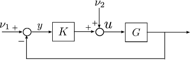
Figure 1: Standard unity feedback configuration

We adopt the following notation:

$\mathbb{R}(\lambda)$	Set of all real–rational transfer functions.
$\mathbb{R}(\lambda)^{n\times q}$	Set of $n\times q$ matrices with entries in $\mathbb{R}(\lambda)$ .
TFM	Transfer function matrix, or, equivalently, $\bigcup_{n,q}\mathbb{R}(\lambda)^{n\times q}$.
$\Omega$	Stability region for TFMs.
$\mathbb{A}(\lambda)$	Subset of $\mathbb{R}(\lambda)$ whose entries have poles in $\Omega$.
$\mathbb{A}(\lambda)^{n\times q}$	Set of $n\times q$ stable TFMs.
$\bar{\mathbb{A}}(\lambda)$	Set of stable TFMs, or, equivalently, $\bigcup_{n,q}\mathbb{A}(\lambda)^{n\times q}$.
$\mathbb{B}$	The set $\{0,1\}$.

We also adopt the following assumptions and conventions:

$m$	Dimension of $y$.
$p$	Dimension of $u$.
$G$	The plant is a TFM with strictly proper entries.
$K$	The LTI controller is an element of $\mathbb{R}(\lambda)^{p\times m}$.
$H(G,K)$	The TFM from $\displaystyle[\nu_{1}^{T}\;\;\nu_{2}^{T}\;\>]^{T}$ to $\displaystyle[y^{T}\;\;u^{T}\;\>]^{T}$.
$\otimes$	Kronecker product.
$\overline{1,q}$	$\{1,2,\cdots,q\}$

The indeterminate $\lambda$ is either $s$ for continuous–time or $z$ for discrete–time systems, respectively. The $\lambda$ argument of a TFM is often omitted when its presence is clear from the context. If the transfer matrix $H(G,K)$ is stable we say that $K$ is a stabilizing controller of $G$, or equivalently that $K$ stabilizes $G$. If a stabilizing controller of $G$ exists, we say that $G$ is stabilizable.

II-A Coprime and Doubly Coprime Factorizations for LTI Systems

A right coprime factorization (RCF) of $G$ over $\Omega$ is a fractional representation of the form $G=NM^{-1}$, with $N\in\mathbb{A}^{m\times p}$ and $M\in\mathbb{A}^{p\times p}$, and for which there exist $X\in\mathbb{A}^{p\times m}$ and $Y\in\mathbb{A}^{p\times p}$ satisfying ${Y}M+{X}N=I$ ([3, Ch. 4, Corollary 17]). Analogously, a left coprime factorization (LCF) of $G$ (over $\Omega$) is defined by $G=\widetilde{M}^{-1}\widetilde{N}$, with $\widetilde{N}\in\mathbb{A}^{m\times p}$ and $\widetilde{M}\in\mathbb{A}^{m\times m}$, satisfying $\widetilde{M}\widetilde{Y}+\widetilde{N}\widetilde{X}=I$ for $\widetilde{X}\in\mathbb{A}^{p\times m}$ and $\widetilde{Y}\in\mathbb{A}^{m\times m}$. Due to the natural interpretation of the coprime factorizations as fractional representations, the invertible $\widetilde{M}$ and $M$ factors are sometimes called the “denominator” TFMs of the coprime factorization.

Definition II.1.

A collection of eight stable TFMs $\big{(}M,N$, $\widetilde{M},\widetilde{N}$, $X,Y$, $\widetilde{X},\widetilde{Y}\big{)}$ is called a doubly coprime factorization (DCF) of $G$ over $\Omega$ if $\widetilde{M}$ and $M$ are invertible, yield the following factorizations:

$$G=\widetilde{M}^{-1}\widetilde{N}=NM^{-1}$$

and satisfy the following equality (Bézout’s identity):

$$\left[\begin{array}[]{cc}Y&X\\ -\widetilde{N}&\widetilde{M}\end{array}\right]\left[\begin{array}[]{cc}M&-\widetilde{X}\\ N&\widetilde{Y}\end{array}\right]=I_{m+p}.$$ (1)

To avoid excessive terminology, we refer to doubly coprime factorizations over $\Omega$ simply as doubly coprime factorizations (DCFs) [3, Ch.4, Remark pp. 79].

Theorem II.2.

(Youla) [3, Ch.5, Theorem 1] Let $\big{(}M,N$, $\widetilde{M},\widetilde{N}$, $X,Y$, $\widetilde{X},\widetilde{Y}\big{)}$ be a DCF of $G$. Any stabilizing controller can be written as:

$$K_{Q}=\widetilde{X}_{Q}\widetilde{Y}_{Q}^{-1}=Y_{Q}^{-1}X_{Q}\\$$ (2)

for some $Q$ in $\mathbb{A}^{p\times m}$, where $X_{Q}$, $\widetilde{X}_{Q}$, $Y_{Q}$ and $\widetilde{Y}_{Q}$ are defined as:

$$X_{Q} \overset{def}{=} X+Q\widetilde{M}$$ (3)

$$\widetilde{X}_{Q} \overset{def}{=} \widetilde{X}+MQ$$ (4)

$$Y_{Q} \overset{def}{=} Y-Q\widetilde{N}$$ (5)

$$\widetilde{Y}_{Q} \overset{def}{=} \widetilde{Y}-NQ$$ (6)

It also holds that $K_{Q}$ stabilizes $G$ for any $Q$ in $\mathbb{A}^{p\times m}$.

Remark II.3.

The following identity shows that $\big{(}M,N,\widetilde{M},\widetilde{N},X_{Q},Y_{Q},\widetilde{X}_{Q},\widetilde{Y}_{Q}\big{)}$ in Theorem II.2 is also a DCF of $G$:

$$\left[\begin{array}[]{cc}(Y-Q\widetilde{N})&(X+Q\widetilde{M})\\ -\widetilde{N}&\widetilde{M}\end{array}\right]\left[\begin{array}[]{cc}M&-(\widetilde{X}+MQ)\\ N&(\widetilde{Y}-NQ)\end{array}\right]=I_{m+p},\qquad Q\in\mathbb{A}^{p\times m}$$ (7)

III Feedback Control subject to Sparsity Constraints

The precise formulation of the sparsity constrained stabilization problem is achieved by imposing a certain pre–selected sparsity pattern on the set of admissible stabilizing controllers.

III-A Specifications of Sparsity Constraints on LTI Controllers

For the boolean algebra, the operations $(+,\cdot)$ are defined as usual: $0+0=0\cdot 1=1\cdot 0=0\cdot 0=0$ and $1+0=0+1=1+1=1\cdot 1=1$. By a binary matrix we mean a matrix whose entries belong to the set $\mathbb{B}$. With the usual extension of notation, $\mathbb{B}^{q\times l}$ stands for the set of all binary matrices with $q$ rows and $l$ columns. The addition and multiplication of binary matrices is carried out in the usual way, keeping in mind that the binary operations $(+,\cdot)$ follow the boolean algebra. Binary matrices are marked with a “$\mathrm{bin}$” superscript, in order to distinguish them from transfer function matrices over $\mathbb{R}(\lambda)$. Furthermore, for binary matrices of the same dimension, the notation $\displaystyle A^{\mathrm{{bin}}}\leq B^{\mathrm{{bin}}}$ means that $a_{ij}\leq b_{ij}$ holds entrywise for all $i$ and $j$.

A binary matrix may be associated with a TFM of the same dimension, whereby each entry of the binary matrix corresponds to an entry of the TFM. The following definitions introduce operators that will be used to establish a correspondence between binary matrices and the sparsity pattern of $G$ or sparsity constraints imposed on $K$.

Definition III.1.

(Pattern operator) Given $A$ in $\mathbb{R}(\lambda)^{q\times l}$, we define $\wp(A)\in\mathbb{B}^{q\times l}$ as follows:

$$\wp(A)_{ij}\overset{def}{=}\left\{\begin{array}[]{l}0\quad\mathrm{if}\qquad A_{ij}=0\\ 1\quad\mathrm{otherwise}\end{array}\right.\qquad i,j\in\overline{1,q}\times\overline{1,l}$$ (8)

Definition III.2.

(Sparse operator) Conversely, for any binary matrix $\displaystyle A^{\mathrm{{bin}}}$ in $\mathbb{B}^{q\times l}$, we define the following linear subspace:

$$\mathbb{S}(A^{\mathrm{{bin}}})\overset{def}{=}\Big{\{}A\in\mathbb{R}(\lambda)^{q\times l}\big{|}\;\wp(A)\leq A^{\mathrm{{bin}}}\Big{\}}$$ (9)

Definition III.3.

Given $K^{\mathrm{bin}}$ in $\mathbb{B}^{p\times m}$, the sparsity constraint $\mathcal{S}$ is defined as [10]:

$$\mathcal{S}\overset{def}{=}\mathbb{S}(K^{\mathrm{bin}}),$$ (10)

Hence, $\mathcal{S}$ is the subspace of all controllers $\displaystyle K$ in $\displaystyle\mathbb{R}(\lambda)^{p\times m}$ for which $K_{ij}=0$ whenever $\displaystyle K^{\mathrm{{bin}}}_{ij}=0$.

We assume that $\mathbb{S}$ and $\wp$ act on $G$ and $G^{\mathrm{bin}}$ on an analogous way as above, leading to the following definitions.

Definition III.4.

The following is the sparsity pattern of $G$ ($G^{\mathrm{bin}}\in\mathbb{B}^{m\times p}$):

$$G^{\>\mathrm{bin}}\overset{def}{=}\>\wp(G)$$ (11)

Remark III.5.

From matrix multiplication (in the boolean algebra), we conclude that the following holds:

$$\wp(K\>G)\leq\wp(K)\>\wp(G)$$ (12)

III-B Quadratic Invariance

Definition III.6.

[10, Definition 2] The sparsity constraint $\mathcal{S}$ is called quadratically invariant (QI) under the plant $G$ if

$$KGK\in\mathcal{S},\quad K\>\in\mathcal{S}.$$ (13)

Remark III.7.

The following conditions are equivalent to (13) [10]:

• $\wp(KGK)\leq K^{\mathrm{bin}},\text{ }K\in\mathcal{S}$

• $K^{\mathrm{bin}}G^{\mathrm{bin}}K^{\mathrm{bin}}\leq K^{\mathrm{bin}}$

Definition III.8.

Define the feedback transformation $h_{G}:\mathbb{R}(\lambda)^{p\times m}\rightarrow\mathbb{R}(\lambda)^{p\times m}$ of $G$ with $K$, as follows:

$$h_{G}(K)\overset{def}{=}K\big{(}I+GK\big{)}^{-1},\qquad K\in\mathbb{R}(\lambda)^{p\times m}$$ (14)

Remark III.9.

The feedback transformation $h_{G}(\cdot)$ is invertible, and its inverse is given by

$$h^{-1}_{G}(K)\overset{def}{=}K\big{(}I-GK\big{)}^{-1}$$ (15)

Proof.

Note that $h_{G}(\cdot)$ is well–posed because $K$ is proper and $G$ is strictly proper. The rest of the proof follows by direct algebraic computations and is omitted for brevity. ∎

The following result is used throughout the paper.

Theorem III.10.

[10, Theorem 14] Given a sparsity constraint $\mathcal{S}$, the following equivalence holds:

$$\mathcal{S}\;\text{is QI under}\;G\Longleftrightarrow h_{G}(\mathcal{S})=\mathcal{S}$$ (16)

where we adopt the following abuse of notation:

$$h_{G}(\mathcal{S})\overset{def}{=}\{h_{G}(K)|K\in\mathcal{S}\}$$

An alternative algebraic proof of Theorem (16) is given in [20, Theorem 9].

Remark III.11.

The set $\mathcal{S}$ is QI under the given plant $G$ if and only if $\mathcal{S}$ is QI under $-G$. This implies, via (16) above, that $\mathcal{S}$ is QI under $G$ if and only if $\displaystyle h^{-1}_{G}(\mathcal{S})=\mathcal{S}$, where $h^{-1}_{G}(\mathcal{S})\overset{def}{=}\{h^{-1}_{G}(K)|K\in\mathcal{S}\}$.

IV Main Result

Given a QI sparsity constraint $\mathcal{S}$, in Theorem IV.2 we develop necessary and sufficient conditions for the existence of a stabilizing controller in $\mathcal{S}$. These conditions are formulated in terms of the existence of a doubly coprime factorization of the plant in which the factors satisfy additional constraints. Such a factorization (when it exists) is equivalent to solving an exact model matching problem with stability [17] restrictions, which has been previously investigated in the control literature. The following preparatory result will be used throughout this Section.

Proposition IV.1.

Let $\big{(}M,N,\widetilde{M},\widetilde{N},X,Y,\widetilde{X},\widetilde{Y}\big{)}$ be a given DCF of $G$. The following identities hold:

$$MX_{Q}=K_{Q}\big{(}I+GK_{Q}\big{)}^{-1},\quad\widetilde{X}_{Q}\widetilde{M}=K_{Q}\big{(}I+GK_{Q}\big{)}^{-1},\qquad Q\in\mathbb{A}^{p\times m}$$ (17)

Proof.

We proceed to verifying that $MX_{Q}=K_{Q}\big{(}I+GK_{Q}\big{)}^{-1}$ is true, while the proof that $X_{Q}\widetilde{M}=K_{Q}\big{(}I+GK_{Q}\big{)}^{-1}$ holds is omitted because it is analogous. From $K_{Q}=Y_{Q}^{-1}X_{Q}$ and $G=NM^{-1}$, we get that $K_{Q}\big{(}I+GK_{Q}\big{)}^{-1}=\big{(}I+Y_{Q}^{-1}X_{Q}NM^{-1}\big{)}^{-1}Y_{Q}^{-1}X_{Q}$, where we used the fact that $K_{Q}\big{(}I+GK_{Q}\big{)}^{-1}=\big{(}I+K_{Q}G\big{)}^{-1}K_{Q}$. Finally, using Bézout’s identity we find that $\big{(}I+Y_{Q}^{-1}X_{Q}NM^{-1}\big{)}^{-1}=\big{(}I+Y_{Q}^{-1}(I-Y_{Q}M)M^{-1}\big{)}^{-1}=MY_{Q}$, which by direct substitution in $\big{(}I+Y_{Q}^{-1}X_{Q}NM^{-1}\big{)}^{-1}Y_{Q}^{-1}X_{Q}$ concludes the proof. ∎

The following Theorem is a main result of this paper.

Theorem IV.2.

Let $\big{(}M,N$, $\widetilde{M},\widetilde{N}$, $X,Y$, $\widetilde{X},\widetilde{Y}\big{)}$ be a DCF of $G$ and $\mathcal{S}$ be a QI sparsity constraint.

• Sufficiency: If $Q$ in $\mathbb{A}^{p\times m}$ is such that at least one of the following inequalities holds:

  $$\wp(\widetilde{X}_{Q}\widetilde{M})\leq K^{\mathrm{bin}}$$ (18a)

  $$\wp(MX_{Q})\leq K^{\mathrm{bin}}$$ (18b)

  then $K_{Q}$ is a stabilizing controller in $\mathcal{S}$.

• Necessity: If there is a stabilizing controller in $\mathcal{S}$ then there exists some $Q$ in $\mathbb{A}^{p\times m}$ for which both inequalities in (18) hold and, in addition, the controller can be written as $K_{Q}$.

Proof.

Necessity: Suppose that there exists a stabilizing controller in $\mathcal{S}$, then, as a consequence of Youla’s Theorem II.2, such a controller can be written as $K_{Q}$ for some $Q$ in $\mathbb{A}^{p\times m}$. We now use the fact that $K_{Q}$ is in $\mathcal{S}$ to prove that both inequalities in (18) hold. According to Proposition IV.1 we get from (17) that

$$\widetilde{X}_{Q}\widetilde{M}=K_{Q}\big{(}I+GK_{Q}\big{)}^{-1}$$ (19)

We apply the $\wp$ operator (8) on both sides of equation (19) and using Definition III.8 we find that $\wp(\widetilde{X}_{Q}\widetilde{M})=\wp(h_{G}(K_{Q}))$. Since $\mathcal{S}$ is QI and $K_{Q}$ is in $\mathcal{S}$, it follows from (16) that $h_{G}(K_{Q})$ belongs to $\mathcal{S}$ and $\wp(h_{G}(K_{Q}))\leq K^{\mathrm{bin}}$, which leads to $\wp(\widetilde{X}_{Q}\widetilde{M})\leq K^{\mathrm{bin}}$. Similarly, we employ (17) to get that $\wp(MX_{Q})=\wp(h_{G}(K_{Q}))$ in order to finally obtain that $\wp(MX_{Q})\leq K^{\mathrm{bin}}$.

Sufficiency: Take each side of (19) as an argument for $h_{G}^{-1}(\cdot)$ in order to get via Definition III.8 that $h_{G}^{-1}(\widetilde{X}_{Q}\widetilde{M})=h_{G}^{-1}(h_{G}(K_{Q}))$ and equivalently that $K_{Q}=h_{G}^{-1}(\widetilde{X}_{Q}\widetilde{M})$. In addition, it follows from Remark III.9 and Remark III.11 that $h_{G}^{-1}(\mathcal{S})=\mathcal{S}$, which, from the assumption that $\wp(\widetilde{X}_{Q}\widetilde{M})\leq K^{\mathrm{bin}}$, implies that $K_{Q}=h_{G}^{-1}(\widetilde{X}_{Q}\widetilde{M})$ is in $\mathcal{S}$ . The fact that $K_{Q}$ is stabilizing follows from Youla’s Theorem II.2. The sufficiency with respect to $\wp(MX_{Q})\leq K^{\mathrm{bin}}$ follows by a similar line of proof and so is omitted for brevity. ∎

IV-A Controller Synthesis as An Exact Model–Matching Problem with Stability Restrictions

Henceforth, given a matrix $V$ with $n$ rows and $q$ columns, we adopt the following notation:

$\mathrm{vec}(V)$	$\vec{v}=\mathrm{vec}(V)$ gives $\vec{v}_{(i+(j-1)n)}=V_{i,j}$
$\mathrm{diag}(V)$	$\Delta=\mathrm{diag}(V)$ is diagonal and $\Delta_{ii}=\vec{v}_{i}$

In this section, we will outline a method (based on Theorem IV.2 above) for the computation of a stabilizing controller subject to a pre-selected QI sparsity constraint $\mathcal{S}$ (whenever such a controller exists). Given a DCF of $G$, which can be computed using the standard state–space techniques in [15, 16], our goal is to obtain $Q$ in $\mathbb{A}^{p\times m}$ such that (18) is satisfied.

Our approach is based on the realization that (18) can be cast as the feasibility of an exact model-matching problem [17] with respect to $Q$ in $\mathbb{A}^{p\times m}$. This correspondence is stated precisely in the following Theorem, while Section IV-A1 provides more details and references on the computation and tests for the existence of solutions of the exact model matching problem.

Theorem IV.3.

Consider that a DCF of $G$ $(M,N,\widetilde{M},\widetilde{N},X,Y,\widetilde{X},\widetilde{Y})$ is given and that a QI sparsity constraint $\mathcal{S}$ is pre-selected via a choice of $K^{bin}$ in $\mathbb{B}^{p\times m}$. The existence of a stabilizing controller in $\mathcal{S}$ is equivalent to the existence of $Q$ in $\mathbb{A}^{p\times m}$ for which at least one of the following equivalent equalities holds:

$$\Phi\big{(}M^{T}\otimes\widetilde{M}\big{)}\mathrm{vec}(Q)+\Phi\>\mathrm{vec}\big{(}\widetilde{X}\widetilde{M}\big{)}=0$$ (20a)

$$\Phi\big{(}M^{T}\otimes\widetilde{M}\big{)}\mathrm{vec}(Q)+\Phi\>\mathrm{vec}\big{(}MX\big{)}=0$$ (20b)

where $\Phi$ is defined as:

$$\Phi\overset{def}{=}I-\mathrm{diag}(K^{\mathrm{bin}})$$ (21)

In addition, if there is $Q$ in $\mathbb{A}^{p\times m}$ that satisfies (20) then $K_{Q}$ is a stabilizing controller in $\mathcal{S}$.

Proof.

The proof follows by establishing an equivalence between (20) and (18). We start by rewriting (18) as follows:

$$\wp\big{(}(\widetilde{X}+MQ)\widetilde{M})=\wp\big{(}MQ\widetilde{M}+\widetilde{X}\widetilde{M})\leq K^{\mathrm{bin}}$$ (22)

$$\wp\big{(}M(X+Q\widetilde{M})\big{)}=\wp\big{(}MQ\widetilde{M}+MX)\leq K^{\mathrm{bin}}$$ (23)

The vectorization of (22)-(23) leads to:

$$\wp\bigg{(}\big{(}M^{T}\otimes\widetilde{M}\big{)}\mathrm{vec}(Q)+\mathrm{vec}\big{(}\widetilde{X}\widetilde{M}\big{)}\bigg{)}\leq\mathrm{vec}\big{(}K^{\mathrm{bin}}\big{)}$$ (24)

$$\wp\bigg{(}\big{(}M^{T}\otimes\widetilde{M}\big{)}\mathrm{vec}(Q)+\mathrm{vec}\big{(}MX\big{)}\bigg{)}\leq\mathrm{vec}\big{(}K^{\mathrm{bin}}\big{)}$$ (25)

Now notice that if the $i$-th entry of $\mathrm{vec}\big{(}K^{\mathrm{bin}}\big{)}$ is zero then the corresponding entries of the left hand side of (24) and (25) must both be zero, which is equivalent to (20) ∎

IV-A1 Computational considerations

Problems of the type (20) are of particular importance in linear control theory and were formulated and proposed for the first time by Wolovich ([17]), who also coined the term exact model–matching in the early 1970’s. Under the additional constraint that $Q$ lies in $\mathbb{A}^{p\times m}$, the problem is referred to as exact model–matching with stability restrictions (see [21]). Reliable and efficient state–space algorithms for solving (20) are available in [22], which also describes a method to ascertain when a solution exists and consequently, from Theorem IV.3, decide when a stabilizing controller in $\mathcal{S}$ exists. Given a stabilizing controller in $\mathcal{S}$ one can use the results in [13, 23] to obtain a convex parametrization of all stabilizing controllers in $\mathcal{S}$. Also, since the resulting convex parametrization is affine in $Q$, one can use the tractable methods proposed in [10] to design norm-optimal controllers for both the disturbance attenuation and the mixed–sensitivity $\mathcal{H}_{2}$ problems.

IV-B A Numerical Example

Consider the following choices for the plant $G$ and the QI sparsity constraint $\mathcal{S}$ to be imposed on the controller as specified via $K^{\mathrm{bin}}$:

$$G=\left[\begin{array}[]{cc}\frac{1}{\lambda+4}&\frac{1}{\lambda-2}\\ \frac{1}{\lambda-1}&0\\ \frac{1}{\lambda+5}&\frac{1}{\lambda-3}\end{array}\right]$$

$$K^{\mathrm{bin}}=\left[\begin{array}[]{ccc}0&1&0\\ 1&1&1\\ \end{array}\right]$$

We use the state–space formulas from [15, 16] to obtain the following DCF of $G$:

$$\widetilde{M}=\left[\begin{array}[]{ccc}\frac{\lambda-2}{\lambda+6}&0&0\\ 0&\frac{\lambda-1}{\lambda+7}&\frac{\lambda-3}{\lambda+7}\\ 0&0&\frac{\lambda-3}{\lambda+8}\end{array}\right],\quad\widetilde{N}=\left[\begin{array}[]{cc}\frac{\lambda-2}{(\lambda+4)(\lambda+6)}&\frac{1}{\lambda+6}\\ \frac{2(\lambda+1)}{(\lambda+5)(\lambda+7)}&\frac{1}{\lambda+7}\\ \frac{\lambda-3}{(\lambda+8)(\lambda+5)}&\frac{1}{\lambda+8}\\ \end{array}\right],$$

$$X=\left[\begin{array}[]{ccc}\frac{\lambda-2}{\lambda+6}&\frac{1}{\lambda+7}&\frac{\lambda-3}{\lambda+8}\\ \frac{1}{\lambda+6}&\frac{\lambda-1}{\lambda+7}&\frac{1}{\lambda+8}\\ \end{array}\right],$$

$$Y=\left[\begin{array}[]{cc}\frac{\lambda^{5}+42\lambda^{4}+617\lambda^{3}+4144\lambda^{2}+12968\lambda+15256}{\lambda^{5}+30\lambda^{4}+355\lambda^{3}+2070\lambda^{2}+5944\lambda+6720}&\frac{\lambda^{4}+777\lambda^{3}+9557\lambda^{2}+27300\lambda-13060}{\lambda^{5}+30\lambda^{4}+355\lambda^{3}+2070\lambda^{2}+5944\lambda+6720}\\ \frac{2\lambda+14}{\lambda^{2}+14\lambda+48}&\frac{\lambda^{2}+40\lambda-108.002}{\lambda^{2}+14\lambda+48}\end{array}\right],$$

$$N=\left[\begin{array}[]{cc}\frac{\lambda-1}{(\lambda+4)(\lambda+9)}&\frac{\lambda-3}{(\lambda+10)(\lambda+11)}\\ \frac{1}{\lambda+9}&0\\ \frac{\lambda-1}{(\lambda+5)(\lambda+9)}&\frac{\lambda-2}{(\lambda+10)(\lambda+11)}\\ \end{array}\right],\quad M=\left[\begin{array}[]{cc}\frac{\lambda-1}{\lambda+9}&0\\ 0&\frac{(\lambda-2)(\lambda-3)}{(\lambda+10)(\lambda+11)}\end{array}\right].$$

The remaining factors $\widetilde{X}$ and $\widetilde{Y}$ of the DCF are not needed here. We now proceed to finding a solution for (20), which, according to Theorem IV.3, leads to the conclusion that a stabilizing controller in $\mathcal{S}$ exists. In addition, we will use the aforementioned solution to compute a stabilizing controller.

Since there are two zeros in the sparsity pattern imposed by $K^{\mathrm{bin}}$, the system of equations in (20) has two (nontrivial) equations that are satisfied by the following element of $\mathbb{A}^{p\times m}$:

$$Q=\left[\begin{array}[]{ccc}1&0&1\\ 0&1&\frac{\lambda+8}{\lambda+7}\end{array}\right]$$

The resulting stabilizing central controller $K=Y^{-1}_{Q}X_{Q}$ is given by

$$K=\left[\begin{array}[]{cc}\frac{\lambda+17}{\lambda+7}&0\\ 754\frac{(\lambda+5.87)(\lambda-0.4525)}{(\lambda+4)(\lambda+5)(\lambda+6)(\lambda+8)}&\frac{(\lambda+42.5389)(\lambda-2.5389)}{(\lambda+6)(\lambda+8)}\end{array}\right]^{-1}\left[\begin{array}[]{ccc}0&\frac{1}{\lambda+7}&0\\ \frac{1}{\lambda+6}&0&\frac{1}{\lambda+8}\end{array}\right],$$

which is in $\mathcal{S}$.

IV-C A Youla-like Parametrization of All Sparse, Stabilizing Controllers

In this subsection, we present an alternative statement to Theorem  IV.3 that clarifies the differences between it and Youla’s classical parametrization.

Corollary IV.4.

Let $\mathcal{S}$ be a given QI sparsity constraint and $(M,N,\widetilde{M},\widetilde{N},X,Y,\widetilde{X},\widetilde{Y})$ a DCF of $G$. Assume that there is a stabilizing controller in $\mathcal{S}$ and let $Q_{0}$ in $\mathbb{A}^{p\times m}$ be selected to satisfy (20). Any stabilizing controller in $\mathcal{S}$ can be written as $K_{Q}$, where $Q$ is obtained as:

$$Q=Q_{0}+Q_{\delta}$$ (26)

for some $Q_{\delta}$ in the (convex set) specified by the following inclusions:

$$\mathrm{vec}(Q_{\delta})\in\mathrm{Null}\Big{(}\Phi\big{(}M^{T}\otimes\widetilde{M}\big{)}\Big{)},Q_{\delta}\in\mathbb{A}^{p\times m}$$ (27)

where $\Phi$ is the matrix defined in (21).

Proof.

The proof follows directly from Theorem IV.3. ∎

Corollary IV.4 unveils the fact that once any suitable $Q_{0}$ is found then the set of all stabilizing controllers in $\mathcal{S}$ can be generated from the affine subspace specified by (26)-(27). Notice that in Youla’s classical approach the parameter $Q$ is only required to be in $\mathbb{A}^{p\times m}$, while the additional constraints in (26)-(27) guarantee that the resulting controller will be in $\mathcal{S}$.

IV-D Numerical Considerations

For an introduction to linear subspaces for TFMs and vector bases of such subspaces we refer to [24]. In addition, the authors of [25] describe a systematic, state–space algorithm to determine a basis of the null space of $\Phi\big{(}M^{T}\otimes\widetilde{M}\big{)}$. Note that the main result in [25] enables the computation of a basis having only stable poles, by performing a column compression of the normal rank of $\Phi\big{(}M^{T}\otimes\widetilde{M}\big{)}$ by post–multiplication with a unimodular matrix. Furthermore, this basis is also minimal, in the sense that the basis–matrix, obtained by juxtaposing the basis columns, has no Smith zeros. Hence, this may be used for the parametrization of all stable $\mathrm{vec}(Q)$ in $\mathrm{Null}\Big{(}\Phi\big{(}M^{T}\otimes\widetilde{M}\big{)}\Big{)}$.

For a numerical example illustrating Corollary IV.4, from Subsection IV-C above, we refer to Subsections IV-C and IV-E in [18].

IV-E Norm-Optimal Control Design

We now indicate how Theorem IV.2 can be used in conjunction with results from [10] to design norm-optimal controllers. In particular, given a quadratically invariant sparsity constraint $\mathcal{S}$ one may be interested in solving the following optimization problem:

$$\min_{K\text{stabilizing and }K\in\mathcal{S}}\|H(G,K)\|$$ (28)

where $\|\cdot\|$ is a suitably defined operatorial norm.

Using Theorem IV.2 we can rewrite (28) as follows:

$$\min_{\begin{matrix}(MX+MQ\widetilde{M})\in\mathcal{S}\\ Q\in\mathbb{A}^{p\times m}\end{matrix}}\|H(G,K_{Q})\|$$ (29)

where we used the fact that the inequalities in (18) are equivalent to $\widetilde{X}\widetilde{M}+MQ\widetilde{M}\in\mathcal{S}$ and $MX+MQ\widetilde{M}\in\mathcal{S}$. Notice that Theorem IV.2 guarantees that (28) is feasible if and only if (29) is feasible.

We proceed by noticing that the closed loop TFM for a given controller $K_{Q}$ can be written as:

$$H(G,K_{Q})=\left[\begin{array}[]{cc}\widetilde{Y}\widetilde{M}&-\widetilde{Y}\widetilde{N}\\ \widetilde{X}\widetilde{M}&I-\widetilde{X}\widetilde{N}\end{array}\right]+\left[\begin{array}[]{c}N\\ M\end{array}\right]Q\left[\begin{array}[]{cc}\widetilde{M}&\widetilde{N}\end{array}\right]$$ (30f)

$$=\left[\begin{array}[]{cc}I-NX&-NY\\ MX&MY\end{array}\right]+\left[\begin{array}[]{c}N\\ M\end{array}\right]Q\left[\begin{array}[]{cc}\widetilde{M}&\widetilde{N}\end{array}\right]$$ (30l)

where we used the formulae available in [3, pp.110]. Hence, we can use (29) to rewrite (28) as follows:

$$\min_{\begin{matrix}(MX+MQ\widetilde{M})\in\mathcal{S}\\ Q\in\mathbb{A}^{p\times m}\end{matrix}}\|T_{1}+T_{2}QT_{3}\|$$ (31)

where $T_{1}$, $T_{2}$ and $T_{3}$ are obtained from (30).

The analysis above implies that the sparsity constrained disturbance attenuation problem (as introduced in [10, (1)/pp. 276 ]), or the sparsity constrained mixed $\mathcal{H}^{2}$ sensitivity problem (from [26, pp. 139]) can be solved as a model–matching problem via the numerical technique in [10, Theorem 29].

V Block-decoupling and streamlined solutions

In this Section, we consider that the input and the output vectors of $G$ are partitioned into blocks so that, under certain conditions, $G$ can be factored in a special form that simplifies both the solution of the exact model matching problem of Theorem IV.3 and the parametrization in Corollary IV.4. Henceforward, we consider the following notation:

$r_{y}$	number of partitions of $y$
$\{y_{[i]}\}_{i=1}^{r_{y}}$	partitions of the output vector
$m_{i}$	dimension of $y_{[i]}$

$r_{u}$	number of partitions of $u$
$\{u_{[i]}\}_{i=1}^{r_{u}}$	partitions of the input vector
$p_{i}$	dimension of $u_{[i]}$

The partitions are constructed in a way that the following holds:

$$\begin{matrix}y^{T}&=&\left[y_{[1]}^{T}\cdots y_{[r_{y}]}^{T}\right]^{T},&&\sum_{i=1}^{r_{y}}m_{i}&=&m\\ &&\\ u^{T}&=&\left[u_{[1]}^{T}\cdots u_{[r_{u}]}^{T}\right]^{T},&&\sum_{i=1}^{r_{u}}p_{i}&=&p\end{matrix}$$ (32)

Similarly, we also consider the partitioning of $G$ and $K$ as:

$$\begin{matrix}G&=&\left[\begin{matrix}G_{[11]}&\cdots&G_{[1r_{u}]}\\ \vdots&\ddots&\vdots\\ G_{[r_{y}1]}&\cdots&G_{[r_{y}r_{u}]}\end{matrix}\right]\\ &&\\ K&=&\left[\begin{matrix}K_{[11]}&\cdots&K_{[1r_{y}]}\\ \vdots&\ddots&\vdots\\ K_{[r_{u}1]}&\cdots&K_{[r_{u}r_{y}]}\end{matrix}\right]\end{matrix}$$ (33)

Assumption V.1.

Throughout this Section, we assume that $G$ and an associated partition of the input and output (32) are given.

Remark V.2.

Given factorizations of $G$ and $K$ as $G=\widetilde{M}^{-1}\widetilde{N}=NM^{-1}$ and $K=\widetilde{X}\widetilde{Y}^{-1}=Y^{-1}X$, respectively, the partition in (32) will induce a unique block-partition structure on the factors $N$, $M$, $\widetilde{N}$, $\widetilde{M}$, $X$, $Y$, $\widetilde{X}$ and $\widetilde{Y}$ as well.

V-A Input/Output Decoupled Coprime Factorizations

We start by defining input and output decoupled factorizations for $G$.

Definition V.3.

Let $\widetilde{N}$ and $\widetilde{M}$ be a factorization of $G$. The pair $(\widetilde{N},\widetilde{M})$ is called output decoupled if $\widetilde{M}$ has the following block diagonal structure:

$$\widetilde{M}=\mathrm{diag}(\{\widetilde{M}_{[ii]}\}_{i=1}^{r_{y}})$$ (34)

where $\mathrm{diag}(\{\widetilde{M}_{[ii]}\}_{i=1}^{r_{y}})$ is defined as:

$$\mathrm{diag}(\{\widetilde{M}_{[ii]}\}_{i=1}^{r_{y}})\overset{def}{=}\left[\begin{matrix}\widetilde{M}_{[11]}&0&\cdots&0\\ 0&\widetilde{M}_{[22]}&\cdots&0\\ \vdots&&\ddots&\vdots\\ 0&0&\cdots&\widetilde{M}_{[r_{y}r_{y}]}\end{matrix}\right]$$ (35)

Definition V.4.

Let $N$ and $M$ be a factorization of $G$. The pair $(N,M)$ is called input decoupled if $M$ has the following block diagonal structure:

$$M=\mathrm{diag}(\{M_{[ii]}\}_{i=1}^{r_{u}})$$ (36)

Remark V.5.

Notice that an output decoupled factorization can always be constructed by factoring each block row of $G$ separately as follows:

$$\left[G_{[i1]}\cdots G_{[ir_{u}]}\right]=\widetilde{M}^{-1}_{[ii]}\left[\widetilde{N}_{[i1]}\cdots\widetilde{N}_{[ir_{u}]}\right],\qquad i\in\overline{1,r_{y}}$$ (37)

An input decoupled factorization can also be constructed by factoring the block columns of $G$.

Definition V.6.

A DCF $\big{(}M,N$, $\widetilde{M},\widetilde{N}$, $X,Y$, $\widetilde{X},\widetilde{Y}\big{)}$ of $G$ is called input/output decoupled if the pairs $(N,M)$ and $(\widetilde{N},\widetilde{M})$ are input and output decoupled, respectively.

It is important to notice that the procedure outlined in Remark V.5 does not guarantee that the pairs $(N,M)$ and $(\widetilde{N},\widetilde{M})$ will be co-prime, much less doubly co-prime. In fact, $G$ may not admit an input/output decoupled DCF. Sufficient conditions and algorithms to obtain an input/output decoupled DCF for $G$ are provided in the Appendix I.

There are two substantial benefits of working with an input/output DCF for G: The first is that the constraint on $Q$ in Theorem IV.2 reduces to $Q\in\mathcal{S}\bigcap\mathbb{A}^{p\times m}$, which leads to a parametrization of all stabilizing controllers that has a simpler characterization. The second advantage is that the exact model-matching problem of Theorem IV.3 admits a unique solution that can be easily computed (see Section V-C).

V-B Theorem IV.2 Revisited

Here, we modify the definitions of Section III so that they account for the assumed input/output partition in (32). More specifically, sparsity constraints will be imposed on entire block sub-matrices of $K$. The definitions in Section III can be recovered from the ones below for the case when the block sub-matrices have dimension one, i.e., provided that $r_{y}=m$ and $r_{u}=p$.

Definition V.7.

Given $K$ in $\mathbb{R}(\lambda)^{p\times m}$, we define $\wp(K)\in\mathbb{B}^{r_{u}\times r_{y}}$ as follows:

$$\wp(K)_{ij}\overset{def}{=}\left\{\begin{array}[]{l}0\quad\mathrm{if}\qquad K_{[ij]}=0_{p_{i}\times m_{j}}\\ 1\quad\mathrm{otherwise}\end{array}\right.\qquad i,j\in\overline{1,r_{u}}\times\overline{1,r_{y}}$$ (38)

where $0_{p_{i}\times m_{j}}$ is a matrix with $p_{i}$ rows and $m_{j}$ columns and whose entries are all zero.

Definition V.8.

Conversely, for any binary matrix $\displaystyle K^{\mathrm{bin}}$ in $\mathbb{B}^{r_{u}\times r_{y}}$, we define the following linear subspace:

$$\mathbb{S}(K^{\mathrm{bin}})\overset{def}{=}\Big{\{}K\in\mathbb{R}(\lambda)^{p\times m}\big{|}\wp(K)\leq K^{\mathrm{bin}}\Big{\}}$$ (39)

Definition V.9.

Given $K^{\mathrm{bin}}$ in $\mathbb{B}^{r_{u}\times r_{y}}$, the sparsity constraint $\mathcal{S}$ is defined as:

$$\mathcal{S}\overset{def}{=}\mathbb{S}(K^{\mathrm{bin}}),$$ (40)

Hence, $\mathcal{S}$ is the subspace of all controllers $\displaystyle K$ in $\displaystyle\mathbb{R}(\lambda)^{p\times m}$ for which $K_{[ij]}=0_{p_{i}\times m_{j}}$ whenever $\displaystyle K^{\mathrm{bin}}_{ij}=0$. In addition, we assume that $\mathbb{S}$ and $\wp$ act on $G$ and $G^{\mathrm{bin}}$ as well as on the factors of any DCF of $G$ in an analogous way.

Remark V.10.

As a consequence of the definitions above, the following holds for any input/output decoupled DCF of $G$:

$$\begin{matrix}\wp(M)&=&I_{r_{u}\times r_{u}},&&\wp(N)&\underset{(a)}{\leq}&G^{bin}\\ \wp(\widetilde{M})&=&I_{r_{y}\times r_{y}},&&\wp(\widetilde{N})&\underset{(b)}{\leq}&G^{bin}\end{matrix}$$ (41)

where (a)-(b) follow from (34) and the fact that $G=\widetilde{M}^{-1}N=NM^{-1}$.

The following Corollary is an immediate consequence of Theorem IV.2 and the facts that $\wp(M)=I_{r_{u}\times r_{u}}$, $\wp(\widetilde{M})=I_{r_{y}\times r_{y}}$, and $M^{-1}$ and $\widetilde{M}^{-1}$ are well defined TFMs.

Corollary V.11.

Let $\big{(}M,N$, $\widetilde{M},\widetilde{N}$, $X,Y$, $\widetilde{X},\widetilde{Y}\big{)}$ be an input/output decoupled DCF of $G$ and $\mathcal{S}$ be a QI sparsity constraint.

• Sufficiency: If $Q$ in $\mathbb{A}^{p\times m}$ is such that at least one of the following inequalities holds:

  $$\wp(\widetilde{X}_{Q})\leq K^{\mathrm{bin}}$$ (42a)

  $$\wp(X_{Q})\leq K^{\mathrm{bin}}$$ (42b)

  then $K_{Q}$ is a stabilizing controller in $\mathcal{S}$.

• Necessity: If there is a stabilizing controller in $\mathcal{S}$ then there exists some $Q$ in $\mathbb{A}^{p\times m}$ for which both inequalities in (42) hold and, in addition, the controller can be written as $K_{Q}$.

The following Corollary is the main result of this section.

Corollary V.12.

Let $\mathcal{S}$ be a given QI sparsity constraint and $(M,N,\widetilde{M},\widetilde{N},X,Y,\widetilde{X},\widetilde{Y})$ an input/output decoupled DCF of $G$. Assume that there is a stabilizing controller in $\mathcal{S}$ and let $Q_{0}$ in $\mathbb{A}^{p\times m}$ be selected to satisfy (42). Any stabilizing controller in $\mathcal{S}$ can be written as $K_{Q}$, where $Q$ is obtained as:

$$Q=Q_{0}+Q_{\delta},\qquad Q_{\delta}\in\mathcal{S}\cap\mathbb{A}^{p\times m}$$ (43)

Proof.

From Corollary V.11 and Theorem IV.3, it follows that since $Q_{0}$ satisfies (42) then it will also satisfy (20). Hence, from Corollary IV.4, any stabilizing controller in $\mathcal{S}$ can be written as $K_{Q}$, with $Q=Q_{0}+Q_{\delta}$, where $Q_{\delta}$ satisfies (27). The proof follows from noticing that since $M\otimes\widetilde{M}$ is block diagonal and its inverse is a well defined TFM, $Q$ satisfies (27) if and only if $\mathrm{vec}(Q_{\delta})\in\mathrm{Null}(\Phi)\cap\mathbb{A}^{p\times m}$ holds, or equivalently $Q_{\delta}$ is in $\mathcal{S}\cap\mathbb{A}^{p\times m}$. ∎

V-C Theorem IV.3 revisited

In this subsection, we show that if an input/output decoupled DCF of $G$ exists then we can use Corollary V.11 to obtain a simplified version of Theorem IV.3. A precise statement of this result is given in Corollary V.15.

Definition V.13.

We define the binary matrix $K^{\mathrm{bin}}_{\perp}$ belonging to the set $\mathbb{B}^{r_{u}\times r_{y}}$ as follows:

$$\big{(}{K^{\mathrm{bin}}_{\perp}}\big{)}_{ij}\overset{def}{=}\left\{\begin{array}[]{l}1\quad\mathrm{if}\;K^{\mathrm{bin}}_{ij}=0,\\ 0\quad\mathrm{otherwise}\>.\end{array}\right.$$ (44)

Definition V.14.

Given $\displaystyle K^{\mathrm{{bin}}}_{\perp}\in\mathbb{B}^{r_{u}\times r_{y}}$ we introduce the linear subspace $\mathcal{S}_{\perp}$ of $\displaystyle\mathbb{R}(\lambda)^{p\times m}$ as

$$\mathcal{S}_{\perp}\overset{def}{=}\Big{\{}K\in\mathbb{R}(\lambda)^{p\times m}\Big{|}\>\wp(K)\leq K^{\>\mathrm{bin}}_{\perp}\Big{\}}.$$ (45)

Corollary V.15.

Let $\big{(}M,N$, $\widetilde{M},\widetilde{N}$, $X,Y$, $\widetilde{X},\widetilde{Y}\big{)}$ be an input/output decoupled DCF of $G$. Given a QI sparsity constraint $\mathcal{S}$, $G$ is stabilizable by a controller in $\mathcal{S}$ if and only if $M^{-1}\widetilde{X}_{\mathcal{S}_{\perp}}$ is in $\mathbb{A}^{p\times m}$, where $\widetilde{X}_{\mathcal{S}_{\perp}}$ results from the additive factorization $\widetilde{X}=\widetilde{X}_{\mathcal{S}}+\widetilde{X}_{\mathcal{S}_{\perp}}$ satisfying $\wp(\widetilde{X}_{\mathcal{S}})\leq K^{\mathrm{bin}}$ and $\wp(\widetilde{X}_{\mathcal{S}_{\perp}})\leq K^{\mathrm{bin}}_{\perp}$.

Proof.

We start by restating the first equation of (42) for any $Q$ as:

$$\wp(\widetilde{X}+MQ)=\wp\big{(}\widetilde{X}_{\mathcal{S}}+MQ_{\mathcal{S}}+M(M^{-1}\widetilde{X}_{\mathcal{S}_{\perp}}+Q_{\mathcal{S}_{\perp}})\big{)}\leq K^{\mathrm{bin}}$$ (46)

where $Q=Q_{\mathcal{S}}+Q_{\mathcal{S}_{\perp}}$ and $\wp(Q_{\mathcal{S}})\leq K^{\mathrm{bin}}$ and $\wp(Q_{\mathcal{S}_{\perp}})\leq K^{\mathrm{bin}}_{\perp}$.

We now recall that according to Corollary V.11, $G$ is stabilizable by a controller in $\mathcal{S}$ if and only if there is $Q$ in $\mathbb{A}^{p\times m}$ so that (46) holds. However, given the fact that $M^{-1}$ is block diagonal, (46) holds for some $Q$ in $\mathbb{A}^{p\times m}$ if and only if $M^{-1}\widetilde{X}_{\mathcal{S}_{\perp}}=-Q_{\mathcal{S}_{\perp}}$ has a solution where $Q_{\mathcal{S}_{\perp}}$ is in $\mathbb{A}^{p\times m}$. Since $M^{-1}\widetilde{X}_{\mathcal{S}_{\perp}}=-Q_{\mathcal{S}_{\perp}}$ has a unique solution because $M$ is invertible, we conclude that there exists $Q_{\mathcal{S}_{\perp}}$ is in $\mathbb{A}^{p\times m}$ satisfying (46) if and only if $M^{-1}\widetilde{X}_{\mathcal{S}_{\perp}}$ is in $\mathbb{A}^{p\times m}$. Notice that $\wp(M^{-1}\widetilde{X}_{\mathcal{S}_{\perp}})\leq K^{\mathrm{bin}}_{\perp}$ always holds because $M$ is block diagonal. ∎

VI Conclusions

We address the design of stabilizing controllers subject to a pre-selected quadratically invariant sparsity pattern. We show that the previously unsolved problem of determining stabilizability with sparsity constraints is equivalent to the solvability of an exact model-matching system of equations that is tractable via existing techniques, and we also outline a systematic method to compute an admissible controller. The proposed analysis also leads to a convex parametrization that is an extension of Youla’s classical result so as to incorporate sparsity constraints on the set of stabilizing controllers. We indicate how this parametrization can be used to write sparsity-constrained norm-optimal control problems in convex form.

Appendix I

This Appendix has two parts. In the first part we give a sufficient condition that guarantees the existence of an output (input) decoupled left (right) coprime factorization for $G$, as in Definitions V.3 and V.4. In the second part, we show that if $G$ admits the aforementioned factorizations then there is a state–space method for computing its input/output decoupled DCF of Definition V.6.

VI-A A Sufficient Condition for the Existence of an Output (Input) Decoupled Left (Right) Coprime Factorization

We are given a plant $G$, partitioned as in (33). As described in Remark V.5, we perform a left coprime factorization for each of the $r_{y}$ block–rows of $G$ (such left coprime factorizations always exist and can be computed using the classical state–space methods from [15, 16]) in order to get

$$\left[G_{[i1]}\cdots G_{[ir_{u}]}\right]=\widetilde{M}^{-1}_{[ii]}\left[\widetilde{N}_{[i1]}\cdots\widetilde{N}_{[ir_{u}]}\right],\qquad i\in\overline{1,r_{y}}.$$ (47)

where the poles of $M_{[ii]}$ can be placed anywhere in the stability domain $\Omega$.

The following proposition gives a necessary and sufficient condition under which the row factorizations in (47) can be concatenated to produce a left decoupled coprime factorization for $G$. It should be noted that a left decoupled coprime factorization for $G$ may exist that cannot be constructed from the row factorizations in (47). This indicates that the proposition is only a sufficient condition for the existence of a left decoupled coprime factorization for $G$.

Proposition VI.1.

Let $(\widetilde{M},\widetilde{N})$ be an output decoupled left factorization derived from the row coprime factorizations (47) as follows:

$$\left[\begin{matrix}G_{[11]}&\cdots&G_{[1r_{u}]}\\ \vdots&\ddots&\vdots\\ G_{[r_{y}1]}&\cdots&G_{[r_{y}r_{u}]}\end{matrix}\right]=\left[\begin{matrix}\widetilde{M}^{-1}_{[11]}&\cdots&0\\ \vdots&\ddots&\vdots\\ 0&\cdots&\widetilde{M}^{-1}_{[r_{y}r_{y}]}\\ \end{matrix}\right]\left[\begin{matrix}\widetilde{N}_{[11]}&\cdots&\widetilde{N}_{[1r_{u}]}\\ \vdots&\ddots&\vdots\\ \widetilde{N}_{[r_{y}1]}&\cdots&\widetilde{N}_{[r_{y}r_{u}]}\\ \end{matrix}\right]$$ (48)

and consider $\Psi$ to be the following TFM:

$$\Psi\overset{def}{=}\left[\begin{matrix}\widetilde{M}_{[11]}&\cdots&0&\widetilde{N}_{[11]}&\cdots&\widetilde{N}_{[1r_{u}]}\\ \vdots&\ddots&\vdots&\vdots&&\vdots\\ 0&\cdots&\widetilde{M}_{[r_{y}r_{y}]}&\widetilde{N}_{[r_{y}1]}&\cdots&\widetilde{N}_{[r_{y}r_{u}]}\end{matrix}\right]$$

The following holds:

1. The output decoupled left factorization in (48) is coprime if and only if the following holds:

   $$\operatorname{rank}(\Psi(\lambda))=m,\qquad\lambda\in\Lambda_{G}$$ (49)

   where $\Lambda_{G}$ represents the set of unstable poles of $G$.

2. The condition in (49) does not depend on the choice of the row coprime factorizations (47).

Proof.

The proof follows as a consequence of standard results in linear systems theory, so we only provide a sketch of the ideas. We start by invoking a result used in [27] that the left factorization $(\widetilde{M},\widetilde{N})$ is coprime if and only if $\Psi$ has no Smith zeros in $\mathbb{C}-\Omega$ . Hence, from the statement in 1), we are left to prove that any Smith zero of $\Psi$ in $\mathbb{C}-\Omega$ is a pole of $G$. The proof of 1) is concluded by noticing that if a given $\lambda_{0}$ in $\mathbb{C}-\Omega$ is not a pole of $G$ then, from the coprimeness of the row factorizations in (47), $\widetilde{M}(\lambda_{0})$ is invertible and hence full rank, leading to the conclusion that $\Psi(\lambda_{0})$ must also be full row rank, and hence $\lambda_{0}$ is not a Smith zero of $\Psi$.

It only remains to prove 2). The argument here follows from the fact that the set of all left coprime factorizations of any block–row of $G$ is given by (47) up to a premultiplication by a unimodular TFM [3, Ch. 4, Theorem 43]. This in turn implies that $\Psi(\lambda)$ is unique, up to a premultiplication of a block–diagonal, unimodular TFM (having the same block partition as $\widetilde{M}$), which does not alter the rank condition on $\Psi(\lambda)$ at any unstable $\lambda_{0}\in(\mathbb{C}-\Omega)$. ∎

The corresponding test for the existence of input decoupled right coprime factorization of $G$ (Definition V.4) is analogous and is therefore omitted for brevity.

VI-B A State-Space Method to Compute an Input/Output Decoupled DCF

We assume that $G$ admits an output decoupled left coprime factorization $G=\widetilde{M}^{-1}\widetilde{N}$ and an input decoupled right coprime factorization $G=NM^{-1}$. These factorizations must be pre-computed (using for instance the arguments described in Appendix I- A), so we consider the $\widetilde{M},M,\widetilde{N},N$ factors fixed. Under these conditions, here we provide a computational algorithm to obtain the Input/Output Decoupled DCF of $G$ (Definition V.6), i.e. a DCF

$$\left[\begin{array}[]{cc}Y&X\\ -\widetilde{N}&\widetilde{M}\end{array}\right]\left[\begin{array}[]{cc}M&-\widetilde{X}\\ N&\widetilde{Y}\end{array}\right]=I_{m+p}.$$ (50)

containing the fixed factors $\widetilde{M},M,\widetilde{N},N$. The fact that the coprime factorization (50) always exists is guaranteed by [3, Ch. 4, Theorem 60] but since we are not aware of any method to actually compute it, we will present one here.

The following additional notation is needed: given any $n$–dimensional state–space representation $(A$, $B$, $C$, $D)$ of a LTI system, its input–output description is given by the transfer function matrix (TFM) which is the $m\times p$ matrix with real, rational functions entries

$$G=\left[\begin{array}[]{c|c}A&B\\ \hline\cr C&D\end{array}\right]\overset{def}{=}D+C(\lambda I_{n}-A)^{-1}B,$$ (51)

where $A,B,C,D$ are $n\times n$, $n\times p$, $m\times n$, $m\times p$ real matrices, respectively while $n$ is also called the order of the realization. For elementary notions in linear systems theory, such as controllability, observability, detectability, we refer to [28], or any other standard text book in linear systems.

We have started out with an output decoupled left coprime factorization (Definition V.3) of the plant $G=\widetilde{M}^{-1}\widetilde{N}$. The state–space representation of this left coprime factorization can be obtained according to Proposition VI.3 A) from Appendix II, starting from a certain stabilizable state–space realization of $G$ (which we take without loss of generality to be in the Kalman Structural Decomposition, [29]) and which we consider fixed:

$$G=\left[\begin{array}[]{cccc|c}\star&\star&\star&\star&\star\\ O&A_{22}&O&A_{24}&B_{2}\\ O&O&\star&\star&O\\ O&O&O&A_{44}&O\\ \hline\cr O&C_{2}&O&C_{4}&D\\ \end{array}\right]$$ (52)

with the $\star$ denoting parts of the realizations that are of no importance in this proof. Continuing with Proposition VI.3 A) from Appendix II, there also exists an invertible matrix $U$ and a feedback matrix $F$ (both fixed) such that (with $F$ partitioned in accordance with (52)) we get

$$\left[\begin{array}[]{cc}-\widetilde{N}&\widetilde{M}\end{array}\right]=U{}^{-1}\left[\begin{array}[]{cccc|cc}\star&\star&\star&\star&\star&\star\\ O&A_{22}-F_{2}C_{2}&O&A_{24}-F_{2}C_{4}&B_{2}-F_{2}D&F_{2}\\ O&\star&\star&\star&\star&\star\\ O&-F_{4}C_{2}&O&A_{44}-F_{4}C_{4}&-F_{4}D&F_{4}\\ \hline\cr O&-C_{2}&O&-C_{4}&-D&I\\ \end{array}\right]$$ (53)

with

$$\Lambda\left(\left[\begin{array}[]{cc}A_{22}-F_{2}C_{2}&A_{24}-F_{2}C_{4}\\ -F_{4}C_{2}&A_{44}-F_{4}C_{4}\\ \end{array}\right]\right)\subset\Omega.$$ (54)

Note that since (52) is stabilizable it follows that $\Lambda(A_{44})\subset\Omega$. After removing the unobservable part from (53) we get that

$$\left[\begin{array}[]{cc}-\widetilde{N}&\widetilde{M}\end{array}\right]=U{}^{-1}\left[\begin{array}[]{cc|cc}A_{22}-F_{2}C_{2}&A_{24}-F_{2}C_{4}&B_{2}-F_{2}D&F_{2}\\ -F_{4}C_{2}&A_{44}-F_{4}C_{4}&-F_{4}D&F_{4}\\ \hline\cr-C_{2}&-C_{4}&-D&I\\ \end{array}\right]$$ (55)

We have also started out with an input decoupled right coprime factorization (Definition V.4) $G=NM^{-1}$. According to Proposition VI.3 B) in Appendix II, there exists a certain detectable state–space realization of $G$ (which we take without loss of generality to be in the Kalman Structural Decomposition) and which we also consider fixed:

$$G=\left[\begin{array}[]{cccc|c}A_{11}&A_{12}&\star&\star&B_{1}\\ O&A_{22}&O&\star&B_{2}\\ O&O&\star&\star&O\\ O&O&O&\star&O\\ \hline\cr O&C_{2}&O&\star&D\\ \end{array}\right]$$ (56)

with the $\star$ denoting parts of the realization that are of no importance here. Any two realizations of $G$ will always have the same the controllable and observable part, up to a similarity transformation - that is to say that if the controllable and stabilizable part of (52) is $(A_{22},B_{2},C_{2},D)$ then the controllable and stabilizable part of (56) must be $(Z^{-1}A_{22}Z,Z^{-1}B_{2},$ $C_{2}Z,D)$, for some invertible, real matrix $Z$ . We can apply this similarity transformation adequately on (56), such that the the controllable and stabilizable part $(A_{22},B_{2},C_{2},D)$, appears identical on both realizations (52) and (56), respectively. This simplifies future computations.

According to Proposition VI.3 B) from Appendix II, along with realization (56), there also exists an invertible matrix $V$ and a feedback matrix $L$ (both fixed) such that (with $L$ partitioned in accordance with (56))

$$\left[\begin{array}[]{c}M\\ N\\ \end{array}\right]=\left[\begin{array}[]{cccc|c}A_{11}-B_{1}L_{1}&A_{12}-B_{1}L_{2}&\star&\star&B_{1}\\ -B_{2}L_{1}&A_{22}-B_{2}L_{2}&\star&\star&B_{2}\\ O&O&\star&\star&O\\ O&O&O&\star&O\\ \hline\cr-L_{1}&-L_{2}&\star&\star&I\\ -DL_{1}&C_{2}-DL_{2}&\star&\star&D\\ \end{array}\right]V$$ (57)

with

$$\Lambda\left(\left[\begin{array}[]{cc}A_{11}-B_{1}L_{1}&A_{12}-B_{1}L_{2}\\ -B_{2}L_{1}&A_{22}-B_{2}L_{2}\end{array}\right]\right)\subset\Omega,$$ (58)

Note that since (56) is detectable it follows that $\Lambda(A_{11})\subset\Omega$. After removing the uncontrollable part from (57) we get that

$$\left[\begin{array}[]{c}M\\ N\\ \end{array}\right]=\left[\begin{array}[]{cc|c}A_{11}-B_{1}L_{1}&A_{12}-B_{1}L_{2}&B_{1}\\ -B_{2}L_{1}&A_{22}-B_{2}L_{2}&B_{2}\\ \hline\cr-L_{1}&-L_{2}&I\\ -DL_{1}&C_{2}-DL_{2}&D\\ \end{array}\right]V$$ (59)

We have come now to the following stabilizable and detectable state–space realization of $G$, which we consider fixed:

$$G=\left[\begin{array}[]{ccc|c}A_{11}&A_{12}&\star&B_{1}\\ O&A_{22}&A_{24}&B_{2}\\ O&O&A_{44}&O\\ \hline\cr O&C_{2}&C_{4}&D\\ \end{array}\right]$$ (60)

Since $\Lambda(A_{11})\subset\Omega$ we get that (60) is detectable and since $\Lambda(A_{44})\subset\Omega$ we get that (60) is stabilizable, hence (60) satisfies the hypothesis from Theorem VI.2 iii) from Appendix II. Starting from realization (60) (which is fixed), (68) and (69) yield a valid DCF of $G$ for any stabilizing feedback matrices $F^{+}$ and $L^{+}$ (partitioned in accordance with (60) and satisfying Theorem VI.2 ii) from Appendix II), and any invertible matrix $T^{+}$ satisfying the hypothesis of Theorem VI.2 i). We will denote the factors of this particular DCF with $\big{(}M^{+},N^{+}$, $\widetilde{M}^{+},\widetilde{N}^{+}$, $X^{+},Y^{+}$, $\widetilde{X}^{+},\widetilde{Y}^{+}\big{)}$. After removing the unobservable part, the $\widetilde{M}^{+}$ factor will be (the computation are similar with those for getting from (53) to (55))

$$\widetilde{M}^{+}={U^{+}}^{-1}\left[\begin{array}[]{cc|c}A_{22}-F^{+}_{2}C_{2}&A_{24}-F^{+}_{2}C_{4}&F^{+}_{2}\\ -F^{+}_{4}C_{2}&A_{44}-F^{+}_{4}C_{4}&F^{+}_{4}\\ \hline\cr-C_{2}&-C_{4}&I\\ \end{array}\right]$$ (61)

where

$$\Lambda\left(\left[\begin{array}[]{cc}A_{22}-F^{+}_{2}C_{2}&A_{24}-F^{+}_{2}C_{4}\\ -F^{+}_{4}C_{2}&A_{44}-F^{+}_{4}C_{4}\\ \end{array}\right]\right)\subset\Omega.$$ (62)

and $U^{+}$ is a real, invertible matrix. We compute the factor $\widetilde{\Theta}\overset{def}{=}\widetilde{M}{\widetilde{M^{+}}}^{-1}$ using the state–space realizations from (53) and (61) respectively and we get

$$\widetilde{\Theta}=U^{-1}\left[\begin{array}[]{cccc|c}A_{22}-F_{2}C_{2}&A_{24}-F_{2}C_{4}&F_{2}C_{2}&F_{2}C_{4}&F_{2}\\ -F_{4}C_{2}&A_{44}-F_{4}C_{4}&F_{4}C_{2}&F_{4}C_{4}&F_{4}\\ O&O&A_{22}&A_{24}&F^{+}_{2}\\ O&O&O&A_{44}&F^{+}_{4}\\ \hline\cr-C_{2}&-C_{4}&C_{2}&C_{4}&I\\ \end{array}\right]U^{+}.$$ (63)

After removing the unobservable part from (63) we get that

$$\widetilde{\Theta}=U^{-1}\left[\begin{array}[]{cc|c}A_{22}-F_{2}C_{2}&A_{24}-F_{2}C_{4}&F_{2}-F^{+}_{2}\\ -F_{4}C_{2}&A_{44}-F_{4}C_{4}&F_{4}-F^{+}_{4}\\ \hline\cr-C_{2}&-C_{4}&I\\ \end{array}\right]U^{+}$$ (64)

and consequently

$$\widetilde{\Theta}^{-1}={U^{+}}^{-1}\left[\begin{array}[]{cc|c}A_{22}-F^{+}_{2}C_{2}&A_{24}-F^{+}_{2}C_{4}&F_{2}-F^{+}_{2}\\ -F^{+}_{4}C_{2}&A_{44}-F^{+}_{4}C_{4}&F_{4}-F^{+}_{4}\\ \hline\cr C_{2}&C_{4}&I\\ \end{array}\right]U,$$ (65)

which combined with (54) and (62) shows that $\widetilde{\Theta}$ is unimodular. A similar line of reasoning can be used to prove that $\Theta\overset{def}{=}{M^{+}}^{-1}M$ is unimodular.

Finally, compute

$$\Big{(}\left[\begin{array}[]{cc}\Theta^{-1}&O\\ O&\widetilde{\Theta}\end{array}\right]\left[\begin{array}[]{cc}{\widetilde{Y}^{+}}&{\widetilde{X}^{+}}\\ -{\widetilde{N}^{+}}&{\widetilde{M}^{+}}\end{array}\right]\Big{)}\Big{(}\left[\begin{array}[]{cc}M^{+}&-X^{+}\\ N^{+}&Y^{+}\end{array}\right]\left[\begin{array}[]{cc}\Theta&O\\ O&\widetilde{\Theta}^{-1}\end{array}\right]\Big{)}=I_{m+p}$$ (66)

which is still a DCF of $G$ in its own right, due to the unimodularity of $\Theta$ and $\widetilde{\Theta}$. Plugging in the definitions of $\widetilde{\Theta}$ and $\Theta$ into (66) yields

$$\left[\begin{array}[]{cc}\Theta^{-1}{\widetilde{Y}^{+}}&\Theta^{-1}{\widetilde{X}^{+}}\\ -{\widetilde{N}}&{\widetilde{M}}\end{array}\right]\left[\begin{array}[]{cc}M&-X^{+}{\widetilde{\Theta}}^{-1}\\ N&Y^{+}{\widetilde{\Theta}}^{-1}\end{array}\right]=I_{m+p}$$ (67)

which is an input/output decoupled DCF of $G$ and the algorithm ends.

Appendix II

Theorem VI.2.

[30, Theorem 1] Let $G$ be some proper $m\times p$ TFM. The class of all DCFs (1) of $G$ over $\Omega$ is given by

$$\left[\begin{array}[]{cc}M&-\widetilde{X}\\ N&\widetilde{Y}\end{array}\right]=\left[\begin{array}[]{c|cc}A-BL&B&F\\ \hline\cr-L&I&0\\ C-DL&D&I\end{array}\right]T\>,\quad$$ (68)

$$\left[\begin{array}[]{cc}Y&X\\ -\widetilde{N}&\widetilde{M}\end{array}\right]=T^{-1}\left[\begin{array}[]{c|cc}A-FC&B-FD&F\\ \hline\cr L&I&0\\ -C&-D&I\end{array}\right],$$ (69)

where $A,B,C,D,F,L$ and $T$ are real matrices accordingly dimensioned such that

i) $T=\left[\begin{array}[]{cc}V&W\\ O&U\end{array}\right]$ has its diagonal $p\times p$ block $V$ and $m\times m$ block $U$ respectively, invertible,

ii) $F$ and $L$ are feedback–matrices such that $\displaystyle\Lambda(A-BL)\cup\Lambda(A-FC)\subset\Omega$,

iii) $G=\left[\begin{array}[]{c|c}A&B\\ \hline\cr C&D\end{array}\right]$ is a stabilizable and detectable realization.

Corollary VI.3.

Let $G$ be an arbitrary $m\times p$ TFM and $\Omega$ a domain in $\mathbb{C}$.

A) The class of all left coprime factorizations of $G$ over $\Omega$, $G=\widetilde{M}^{-1}\widetilde{N}$, is given by

$$\left[\begin{array}[]{cc}\widetilde{N}&\widetilde{M}\end{array}\right]=U^{-1}\left[\begin{array}[]{c|cc}A-FC&B-FD&-F\\ \hline\cr C&D&I\end{array}\right],$$ (70)

where $A,B,C,D,F$ and $U$ are real matrices accordingly dimensioned such that

i) $U$ is any $m\times m$ invertible matrix,

ii) F is any feedback matrix that allocates the observable modes of the $(C,A)$ pair to $\Omega$,

iii) $G=\left[\begin{array}[]{c|c}A&B\\ \hline\cr C&D\end{array}\right]$ is a stabilizable realization.

B) The class of all right coprime factorizations of $G$ over $\Omega$, $G=NM^{-1}$ is given by

$$\left[\begin{array}[]{c}M\\ N\end{array}\right]=\left[\begin{array}[]{c|c}A-BL&B\\ \hline\cr-L&I\\ C-DL&D\end{array}\right]V$$ (71)

where $A,B,C,D,L$ and $V$ are real matrices accordingly dimensioned such that

i) $V$ is any $p\times p$ invertible matrix,

ii) L is any feedback matrix that allocates the controllable modes of the $(A,B)$ pair to $\Omega$,

iii) $G=\left[\begin{array}[]{c|c}A&B\\ \hline\cr C&D\end{array}\right]$ is a detectable realization.

The proof of Corollary VI.3 follows on the lines of Theorem VI.2.

References

- [1] M. C. Rotkowitz and N. C. Martins, “On the Nearest Quadratically Invariant Information Constraint,” IEEE Transactions on Automatic Control, vol. 57, no. 5, pp. 1314–1319, 2012.
- [2] D. Youla, H. Jabr, and J. J. Bongiorno, “Modern Wiener-Hopf design of optimal controllers–Part II: The multivariable case,” IEEE Transactions on Automatic Control, vol. 21, no. 3, pp. 319–338, 1976.
- [3] M. Vidyasagar, Control System Synthesis: A Factorization Approach. MIT Press, 1985.
- [4] C. A. Desoer, R. W. Liu, J. Murray, and R. Saeks, “Feedback-System Design - the Fractional Representation Approach to Analysis and Synthesis,” IEEE Transactions on Automatic Control, vol. 25, no. 3, pp. 399–412, 1980.
- [5] P. Voulgaris, “Control of nested systems,” in Proceedings of the American Control Conference, 2000, 2000, pp. 4442–4445.
- [6] ——, “A convex characterization of classes of problems in control with specific interaction and communication structures,” in Proceedings of the American Control Conference, 2001., 2001, pp. 3128–3133.
- [7] X. Qi, M. V. Salapaka, P. G. Voulgaris, and M. Khammash, “Structured optimal and robust control with multiple criteria: A convex solution,” IEEE Transactions on Automatic Control, vol. 49, no. 10, pp. 1623–1640, 2004.
- [8] B. Bamieh and P. G. Voulgaris, “A convex characterization of distributed control problems in spatially invariant systems with communication constraints,” Systems & Control Letters, vol. 54, no. 6, pp. 575–583, 2005.
- [9] M. C. Rotkowitz, R. Cogill, and S. Lall, “Convexity of optimal control over networks with delays and arbitrary topology,” Int. J. Systems, Control and Communications, vol. 2, pp. 30–54, Dec. 2010.
- [10] M. C. Rotkowitz and S. Lall, “A characterization of convex problems in decentralized control,” IEEE Transactions on Automatic Control, vol. 51, no. 2, pp. 274–286, 2006.
- [11] ——, “Affine controller parameterization for decentralized control over Banach spaces,” IEEE Transactions on Automatic Control, vol. 51, no. 9, pp. 1497–1500, 2006.
- [12] G. Zames, “Feedback and Optimal Sensitivity - Model-Reference Transformations, Multiplicative Seminorms, and Approximate Inverses,” IEEE Transactions on Automatic Control, vol. 26, no. 2, pp. 301–320, 1981.
- [13] S. Sabău and N. C. Martins, “A convex parameterization of all stabilizing controllers for non-strongly stabilizable plants under quadratically invariant sparsity constraints,” in Proceedings of the American Control Conference, 2009., 2009, pp. 878–883.
- [14] L. Lessard and S. Lall, “Quadratic Invariance is Necessary and Sufficient for Convexity,” American Control Conference (ACC), pp. 5360–5362, 2011.
- [15] C. N. Nett, C. A. Jacobson, and M. J. Balas, “A Connection Between State-Space and Doubly Coprime Fractional Representations,” IEEE Transactions on Automatic Control, vol. 29, no. 9, pp. 831–832, 1984.
- [16] P. Khargonekar and E. D. Sontag, “On the Relation Between Stable Matrix-Fraction Factorizations and Regulable Realizations of Linear-Systems Over Rings,” IEEE Transactions on Automatic Control, vol. 27, no. 3, pp. 627–638, 1982.
- [17] W. A. Wolovich, “The application of state feedback invariants to exact model-matching problems,” in The 5th Annual Princeton Conf. on Inf. Sci., 1971.
- [18] S. Sabau and N. C. Martins, “Necessary and Sufficient Conditions for Stabilizability subject to Quadratic Invariance,” in Decision and Control and European Control Conference (CDC-ECC), 2011 50th IEEE Conference on, 2011, pp. 2459–2466.
- [19] ——, “On the stabilization of lti configurations under quadratically invariant constraints,” in Proceedings of the Forty-Eighth Annual Allerton Conference, 2010, pp. 1004–1010.
- [20] L. Lessard and S. Lall, “An algebraic framework for quadratic invariance,” in Proceedings of the IEEE Conference on Decision and Control (CDC), 2010, 2010, pp. 2698–2703.
- [21] Z. Gao and P. J. Antsaklis, “On Stable-Solutions of the One-Sided and 2-Sided Model-Matching Problems,” IEEE Transactions on Automatic Control, vol. 34, no. 9, pp. 978–982, 1989.
- [22] D. Chu and P. Van Dooren, “A novel numerical method for exact model matching problem with stability,” Automatica, pp. 1697–1704, 2006.
- [23] S. Sabau, “Optimal control with information pattern constraints,” Ph.D. dissertation, University of Maryland, College Park, 2011.
- [24] G. D. Forney, “Minimal Bases of Rational Vector Spaces, with Applications to Multivariable Linear Systems,” SIAM Journal on Control, vol. 13, no. 3, pp. 493–520, May 1975.
- [25] C. Oara and S. Sabau, “Minimal indices cancellation and rank revealing factorizations for rational matrix functions,” Linear Algebra and Its Applications, vol. 431, no. 10, pp. 1785–1814, 2009.
- [26] K. Zhou, J. C. Doyle, and K. Glover, Robust and Optimal Control. Prentice Hall, 1996.
- [27] C. Oara and A. Varga, “Minimal Degree Coprime Factorization of Rational Matrices,” SIAM J Matrix Anal. Appl., vol. 21, no. 1, pp. 245–278, Sep. 1999.
- [28] M. W. Wonham, Linear Multivariable Control. Springer Verlag, 1985.
- [29] R. E. Kalman, “Canonical Structure of Linear Dynamical Systems,” Proceedings of the National Academy of Sciences of the United States of America, vol. 48, pp. 596–600, Apr. 1962.
- [30] V. M. Lucic, “Doubly coprime factorization revisited,” IEEE Transactions on Automatic Control, vol. 46, no. 3, pp. 457–459, 2001.