Restricting exchangeable nonparametric distributions

Abstract

Distributions over exchangeable matrices with infinitely many columns, such as the Indian buffet process, are useful in constructing nonparametric latent variable models. However, the distribution implied by such models over the number of features exhibited by each data point may be poorly-suited for many modeling tasks. In this paper, we propose a class of exchangeable nonparametric priors obtained by restricting the domain of existing models. Such models allow us to specify the distribution over the number of features per data point, and can achieve better performance on data sets where the number of features is not well-modeled by the original distribution.

1 Introduction

The Indian buffet process (IBP)[9] and the related infinite gamma-Poisson process (iGaP)[14] are distributions over matrices with exchangeable rows and infinitely many columns, only a finite (but random) number of which contain any non-zero entries. Such distributions have proved useful for constructing flexible latent factor models that do not require us to specify the number of latent factors a priori. In such models, each column of the random matrix corresponds to a latent feature, and each row to a data point. The non-zero elements of a row select the subset of features that contribute to the corresponding data point.

However, distributions such as the IBP and the iGaP make certain assumptions about the structure of the data that may be inappropriate. Specifically, such priors impose distributions on the number of data points that exhibit a given feature, and on the number of features exhibited by a given data point. For example, in the IBP, the number of features exhibited by a data point is marginally Poisson-distributed, and a feature appears in a new data point with probability $m/(N+1)$, where $N$ is the number of previously seen data points, and $m$ is the number of times that feature has appeared.

These properties may be too constraining for many modeling tasks. There are a number of cases where we might want to increase the flexibility of these models by allowing non-Poisson marginals over the number of latent features per data point, or by adding constraints on the number of features. For example, the IBP has been used to select possible next states in a hidden Markov model [7]. In such a model, we do not expect to see a state that allows no transitions (including self-transitions). Nonetheless, because a data point in the IBP can have zero features with non-zero probability, our prior supports states with no valid transition distribution. Similarly, the iGaP has been used to model features in images [14], and we may wish to exclude the possibility of a featureless image.

One interesting example arises when we expect, or desire, the latent features to correspond to interpretable features, or causes, of the data [16]. We might believe that each data point exhibits exactly $K$ features – corresponding perhaps to speakers in a dialog, members of a team, or alleles in a genotype – but be agnostic about the total number of features in our dataset. A model that explicitly encodes this prior expectation about the number of features per data point will tend to lead to more interpretable and parsimonious results.

In other situations, we may believe that the number of features per data point follows a distribution other than that implied by the IBP. For example, it is well known that text and network data tends to exhibit power-law behavior, suggesting a need for models that impose heavy-tailed distributions on the number of features.

In the case of the IBP, two- and three-parameter extensions have been proposed that modify the distribution over the number of data points that exhibit a feature [13, 8, 12]. While these extensions increase flexibility in the distributions over the number of data points exhibiting each feature, the distribution over the number of features per data point remains Poisson. As we will see, this is an inherent consequence of the use of a completely random measure as both prior and likelihood. In this paper, we consider methods for varying the distribution over the number of features, by removing the completely random assumption.

2 Exchangeability

We say a finite sequence $(X_{1},\dots,X_{N})$ is exchangeable (see, for example, [1]) if its distribution is unchanged under any permutation $\sigma$ of $\{1,\dots,N\}$. Further, we say that an infinite sequence $X_{1},X_{2},\dots$ is infinitely exchangeable if all of its finite subsequences are exchangeable. Such distributions are appropriate when we do not believe the order in which we see our data is important, or when we do not have access to all data points.

De Finetti’s law tells us that a sequence is exchangeable iff the observations are i.i.d. given some latent distribution. This means that we can write the probability of any exchangeable sequence as

$$P(X_{1}=x_{1},X_{2}=x_{2},\dots)=\int_{\Theta}\prod_{i}\mu_{\theta}(X_{i}=x_{i}|\theta)\nu(\theta)d\theta$$ (1)

for some probability distribution $\nu$ over parameter space, and some parametrised family $\{\mu_{\theta}\}_{\theta\in\Theta}$ of conditional probability distributions.

Throughout this paper, we will use the notation $p(x_{1},x_{2},\dots)=P(X_{1}=x_{1},X_{2}=x_{2},\dots)$ to represent the joint distribution over an exchangeable sequence $x_{1},x_{2},\dots$, and $p(x_{n+1}|x_{1},\dots,x_{n})$ to represent the associated predictive distribution. We will also use the notation $p(x_{1},\dots,x_{n},\theta):=\prod_{i=1}^{n}\mu_{\theta}(X_{i}=x_{i}|\theta)\nu(\theta)$ to represent the joint distribution over the observations and the directing measure $\theta$. In general $\theta$ may be infinite dimensional, which motivates the close link between the exchangeability assumption and the need for Bayesian nonparametric models.

2.1 Distributions over exchangeable matrices

The Indian buffet process (IBP)[9] is a distribution over binary matrices with exchangeable rows and infinitely many columns. In the de Finetti representation, the mixing measure $\nu$ is a beta process, and the conditional distribution $\mu_{\theta}$ is a Bernoulli process [13]. The beta process and the Bernoulli process are both completely random measures – distributions over random measures that assign independent masses to disjoint subsets, that can be written in the form $\Gamma=\sum_{k=1}^{\infty}\pi_{k}\delta_{\theta_{k}}$ [11]. In the parametrization of the beta process commonly used for the IBP, the masses of the atoms $\pi_{k}$ of a sample from a beta process can be seen as the infinitesimal limit of $\mbox{Beta}(\alpha dH_{0},1-\alpha dH_{0})$ random variables, for some positive scalar $\alpha$ and CDF $H_{0}$. The masses of the atoms of a sample from a Bernoulli process are distributed according to $\mbox{Bernoulli}(dG_{0})$, for some piecewise-constant function $G_{0}:\mathcal{X}\rightarrow[0,1]$ with an at most countable number of jumps. In the context of the IBP, $G_{0}$ is the cumulative function of the beta-process-distributed measure – so each atom of the beta process gives the probability for a collection of Bernoulli random variables. We can think of the atoms of the beta process as determining the latent probability for a column of a matrix with infinitely many columns, and the Bernoulli process as sampling binary values for the entries of that column of the matrix. The resulting matrix has a finite number of non-zero entries, with the number of non-zero entries in each row distributed as $\mbox{Poisson}(\alpha)$ and the total number of non-zero columns in $N$ rows distributed as $\mbox{Poisson}(\alpha H_{N})$, where $H_{N}$ is the $N$th harmonic number. The number of rows with a non-zero entry for a given column exhibits a “rich gets richer” property – a new row has a one in a given column with probability proportional to the number of times a one has appeared in that column in the preceding rows.

Several models have been formulated that allow us to vary the distribution over the total number of features and the degree to which features are shared between data points. A two-parameter extension of the IBP [10, 13] can be obtained by introducing an extra parameter to the beta process, so that the column probabilities are distributed according to the infinitesimal limit of a $\mbox{Beta}(c\alpha dH_{0},c(1-\alpha dH_{0}))$ distribution. The parameter $c$ controls the degree of sharing of the features in the resulting IBP: As $c\rightarrow 0$, all data points share the same features, and as $c\rightarrow\infty$, all data points have disjoint feature sets. A three-parameter extension [12] replaces the beta process with a completely random measure called the stable-beta process, which includes the beta process as a special case. The resulting IBP exhibits power law behavior: the total number of features exhibited in a dataset of size $N$ grows as $O(N^{s})$ for some $s>0$, and the number of data points exhibiting each feature also follows a power law.

A related distribution over exchangeable matrices is the infinite gamma-Poisson process (iGaP)[14]. Here, the de Finetti mixing measure is the gamma process, and the family of conditional distributions is given by the Poisson process. The atoms of the gamma process correspond to the columns of a matrix, in a manner similar to the beta process in the IBP. In this case, the atoms determine the mean value of the column, and the Poisson process populates the column of the matrix with Poisson random variables with this mean. The result is a distribution over non-negative integer-valued matrices with infinitely many columns and exchangeable rows. The sum of each row is distributed according to a negative binomial distribution.

3 Removing the Poisson assumption

In Section 2.1, we saw that, while existing methods are able to alter the degree of sharing of features and the total number of features in the IBP, they have not been able to remove the Poisson assumption on the number of features per data point. This is noted by Teh and Görür [12], who point out

One aspect of the [three-parameter IBP] which is not power-law is the number of dishes each customer tries. This is simply $\mbox{Poisson}(\alpha)$ distributed. It seems difficult to obtain power-law behavior in this aspect within a CRM framework, because of the fundamental role played by the Poisson process.

To elaborate on this, note that, marginally, the distribution over the value of each element $z_{k}$ of a row $\mathbf{z}$ of the IBP is given by a Bernoulli distribution. Therefore, by the law of rare events, the sum $\sum_{k}z_{k}$ is distributed according to a Poisson distribution. A similar argument applies to the infinite gamma-Poisson process. In general, any distribution over exchangeable random matrices based on a homogeneous CRM will have rows marginally distributed as i.i.d. random variables. In the case of binary matrices, these random variables must be Bernoulli, so their sum will either be Poisson, or infinite. Therefore, in order to circumvent the requirement of a Poisson number of features in an IBP-like model, we must remove the completely random assumption on either the de Finetti mixing measure or the family of conditional distributions.

3.1 Restricting the family of conditional distributions

We are familiar with the idea of restricting the support of a distribution to a measurable subset. For example, a truncated Gaussian is a Gaussian distribution restricted to a certain contiguous section of the real line. In general, we can restrict the support of an arbitrary probability distribution $\mu$ on some space $\Omega$ to a measurable subset $A\subset\Omega$ in the support of $\mu$ by defining $\mu^{|A}(\cdot):=\mu(\cdot)\mathbb{I}(\cdot\in A)/\mu(A)$, where $\mathbb{I}(\cdot)$ is the indicator function.

Theorem 1 (Restricted exchangeable distributions).

We can always restrict the support of an exchangeable distribution on some space by restricting the family of conditional distributions $\{\mu_{\theta}\}_{\theta\in\Theta}$ introduced in Equation 1, to obtain an exchangeable distribution on the restricted space.

Proof.

Consider an unrestricted exchangeable model with de Finetti representation $p(x_{1},\dots,x_{N},\theta)=\prod_{i=1}^{N}\mu_{\theta}(X_{i}=x_{i})\nu(\theta)$. Let $p^{|A}$ be the restriction of $p$ such that $X_{i}\in A,i=1,2,\dots$, obtained by restricting the family of conditional distributions $\{\mu_{\theta}\}$ to $\{\mu_{\theta}^{|A}\}$ as described above. Then

$$p^{|A}(x_{1},\dots,x_{N},\theta)=\prod_{i=1}^{N}\mu_{\theta}^{|A}(X_{i}=x_{i})\nu(\theta)=\prod_{i=1}^{N}\frac{\mu_{\theta}(X_{i}=x_{n})}{\mu_{\theta}(X_{i}\in A)}\nu(\theta)\,,$$

and

$$p^{|A}(x_{N+1}|x_{1},\dots,x_{N})\propto\int_{\Theta}\frac{\prod_{i=1}^{N+1}\mu_{\theta}(X_{i}=x_{i})}{\prod_{i=1}^{N+1}\mu_{\theta}(X_{i}\in A)}\nu(\theta)d\theta$$ (2)

is an exchangeable sequence by construction, according to de Finetti’s law. ∎

We give two examples based on the IBP.

Example 1 (Restriction to a fixed number of non-zero entries per row).

Recall that, conditioned on a latent beta process-distributed measure $B:=\sum_{k}\pi_{k}\delta_{\theta_{k}}$, a sample from the IBP is distributed according to a Bernoulli process. This distribution has support in $\{0,1\}^{\infty}$. We can restrict the support of this Bernoulli process to an arbitrary measurable subset $A\subset\{0,1\}^{\infty}$ – for example, the set of all vectors $\mathbf{z}\in\{0,1\}^{\infty}$ such that $\sum_{k}z_{k}=S$ for some integer $S$. The conditional distribution of a matrix $\mathbf{Z}=\{\mathbf{z}_{1},\dots,\mathbf{z}_{N}\}$ under such a distribution is given by:

$$\mu_{B}^{|S}(Z=\mathbf{Z})=\frac{\prod_{i=1}^{N}\mu_{B}(Z_{i}=\mathbf{z}_{i})\mathbb{I}(\sum_{k}z_{ik}=S)}{(\mu_{B}(\sum_{k}Z_{ik}=S))^{N}}=\frac{\prod_{k=1}^{\infty}\pi_{k}^{m_{k}}(1-\pi_{k})^{N-m_{k}}}{\mbox{PoiBin}(S|\{\pi_{k}\}_{k=1}^{\infty})^{N}}\,,$$ (3)

where $m_{k}=\sum_{n}z_{nk}$ and $\mbox{PoiBin}(\cdot|\{\pi_{k}\}_{k=1}^{\infty})$ is the infinite limit of the Poisson-binomial distribution [4], which describes the distribution over the number of successes in a sequence of independent but non-identical Bernoulli trials. The probability of $\mathbf{Z}$ given in Equation 3 is the infinite limit of the conditional Bernoulli distribution [4], which describes the distribution of the locations of the successes in such a trial, conditioned on their sum.

Example 2 (Restriction to a random number of non-zero entries per row).

Rather than specify the number of non-zero entries in each row a priori, we can allow it to be random, with some arbitrary distribution $f(\cdot)$ over the non-negative integers. A Bernoulli process restricted to have $f$-marginals can be described as

$$\mu_{B}^{|f}(\mathbf{Z})=\prod_{i=1}^{N}\mu_{B}^{|S_{i}}(Z_{i}=\mathbf{z}_{i})f(S_{i})=\bigg{(}\prod_{k=1}^{\infty}\pi_{k}^{m_{k}}(1-\pi_{k})^{N-m_{k}}\bigg{)}\cdot\prod_{i=1}^{N}\frac{f(S_{i})}{\mbox{PoiBin}(S_{i}|\{\pi_{k}\}_{k=1}^{\infty}})\,,$$ (4)

where $S_{n}=\sum_{k}z_{nk}$. Again, if we marginalize over $B$, the resulting distribution is exchangeable, because mixtures of i.i.d. distributions are i.i.d.

We note that, even if we choose $f$ to be $\mbox{Poisson}(\alpha)$, we will not recover the IBP. The IBP has $\mbox{Poisson}(\alpha)$ marginals over the number non-zero elements per row, but the conditional distribution is described by a Poisson-binomial distribution. The Poisson-restricted IBP, however, will have Poisson marginal and conditional distributions.

We also note that the fixed-row-sum model of Example 1 can be seen as a special case of the random-distribution model of Example 2, where the distribution $f$ is degenerate on $S$.

Figure 1 shows some examples of samples from the single-parameter IBP, with parameter $\alpha=5$, with various restrictions applied.

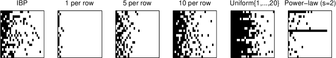
Figure 1: Samples from restricted IBPs.

3.2 Direct restriction of the predictive distributions

The construction in Section 3.1 is explicitly conditioned on a draw $B$ from the de Finetti mixing measure $\nu$. Since it might be cumbersome to explicitly represent the infinite dimensional object $B$, it is tempting to consider constructions that directly restrict the predictive distribution $p(X_{N+1}|X_{1},\dots,X_{N})$, where $B$ has been marginalized out. In other words, can we simply sample from an exchangeable distribution and discard samples that fall outside our region of interest?

We can certainly find examples of exchangeable sequences that remain exchangeable after restricting their conditional distributions:

Example 3 (Infinite gamma-Poisson process).

Consider restricting the predictive distribution of the infinite gamma-Poisson distribution such that each row sums to $S$. In the predictive distribution for the iGaP, for each previously observed feature $k$, we sample an element $X_{nk}\sim\mbox{NegBinom}(m_{k},n/(n+1))$. We then sample a value $N_{n}^{*}\sim\mbox{NegBinom}(\theta,n/(n+1))$ and assign $N_{n}^{*}$ counts to new features according to a Chinese restaurant process. If we restrict this model such that each row sums to $1$, we have:

$$\begin{split}p^{|1}(X_{(N+1)k}=1|X_{1:N})=&\frac{p(X_{(N+1)k}=1|X_{1:N})\prod_{j\neq k}p(X_{(N+1)j}=0|X_{1:N})}{p(\sum_{j}X_{(N+1)j}=1|X_{1:N})}\\ =&\begin{cases}\frac{m_{k}}{\sum_{j}m_{j}+\theta}&\mbox{if feature k has been seen before}\\ \frac{\theta}{\sum_{j}m_{j}+\theta}&\mbox{otherwise.}\end{cases}\end{split}$$

In other words, the infinite gamma-Poisson process restricted to sum to one is a Chinese restaurant process. If we restrict the iGaP to sum to $S$, we have $S$ samples per data point from a Chinese restaurant process.

However, this result does not hold for direct restriction of arbitrary exchangeable sequences.

Theorem 2 (Sequences obtained by directly restricting the predictive distribution of an exchangeable sequence are not, in general, exchangeable.).

Let $p$ be the distribution of the unrestricted exchangeable model introduced in the proof of Theorem 1. Let $p^{*|A}$ be the distribution obtained by directly restricting this unrestricted exchangeable model such that $X_{n}\in A$, i.e.

$$p^{*|A}(x_{N+1}|x_{1},\dots,x_{N})\propto\frac{\int_{\Theta}\prod_{i=1}^{N+1}\mu_{\theta}(X=x_{i})\nu(\theta)d\theta}{\int_{\Theta}\prod_{i=1}^{N+1}\mu_{\theta}(X\in A)\nu(\theta)d\theta}\,.$$ (5)

In general, this will not be equal to Equation 2, and cannot be expressed as a mixture of i.i.d. distributions.

Proof.

To demonstrate that this is true, consider the counterexample given in Example 4. ∎

Example 4 (A three-urn buffet).

Consider a simple form of the Indian buffet process, with a base measure consisting of three unit-mass atoms. We can represent the predictive distribution of such a model using three indexed urns, each containing one red ball (representing a one in the resulting matrix) and one blue ball (representing a zero in the resulting matrix). We generate a sequence of ball sequences by repeatedly picking a ball from each urn, noting the ordered sequence of colors, and returning the balls to their urns, plus one ball of each sampled color.

Proposition 1.

The three-urn buffet is exchangeable.

Proof.

By using the fact that a sequence is exchangeable iff the predictive distribution given the first $N$ elements of the sequence of the $N+1$st and $N+2$nd entries is exchangeable [6], it is trivial to show that this model is exchangeable and that, for example,

$$\begin{split}p(&X_{N+1}=(r,b,r),X_{N+2}=(r,r,b)|X_{1:N})\\ &=\frac{m_{1}m_{2}(N+1-m_{3})}{(N+1)^{3}}\cdot\frac{(m+1+1)(N+1-m_{2})m_{3}}{(N+2)^{3}}\\ &=p(X_{N+1}=(r,r,b),X_{N+2}=(r,b,r)|X_{1:N})\,,\end{split}$$ (6)

where $m_{i}$ is the number of times in the first $N$ samples that the $i$th ball in a sample has been red. ∎

Proposition 2.

The directly restricted three-urn scheme (and, by extension, the directly restricted IBP) is not exchangeable.

Proof.

Consider the same scheme, but where the outcome is restricted such that there is one, and only one, red ball per sample. The probability of a sequence in this restricted model is given by

$$\textstyle p^{*}(X_{N+1}=x|X_{1:N})=\sum_{k=1}^{3}\frac{m_{k}}{N+1-m_{k}}\mathbb{I}(x_{i}=r)\big{/}\sum_{k=1}^{3}\frac{m_{k}}{N+1-m_{k}}$$

and, for example,

$$\begin{split}p^{*}(&X_{N+1}=(r,b,b),X_{N+2}=(b,r,b)|X_{1:N})\\ &=\frac{\frac{m_{1}}{N+1-m_{1}}}{\sum_{k}\frac{m_{k}}{N+1-m_{k}}}\cdot\frac{\frac{m_{2}}{N+2-m_{3}}}{\frac{m_{2}}{N+1-m_{2}}-\frac{m_{2}}{N+2-m_{2}}+\sum_{k}\frac{m_{k}}{N+1-m_{k}}}\\ &\neq p^{*}(X_{N+1}=(b,r,b),X_{N+2}=(r,b,b)|X_{1:N})\,,\end{split}$$ (7)

therefore the restricted model is not exchangeable. By introducing a normalizing constant – corresponding to restricting over a subset of $\{0,1\}^{3}$ – that depends on the previous samples, we have broken the exchangeability of the sequence.

By extension, a model obtained by directly restricting the predictive distribution of the IBP is not exchangeable. ∎

This section shows that, while directly restricting the predictive distribution of the IBP is appealing because it avoids instantiating the infinite latent measure, this construction does not yield an exchangeable distribution. Modifying a Gibbs sampler for the IBP based on the directly restricted predictive distribution would not yield a valid sampler for either the above model, or the exchangeable model described in Section 3.1. For the remainder of the paper, we focus on developing valid sampling schemes for the exchangeable model, which we will refer to as a restricted IBP (rIBP).

4 Inference

In this section, we focus on inference methods for restricted IBPs, since samplers for the restricted iGaP can easily be obtained by modifying existing samplers for the CRP.

We focus on sampling in a truncated model, where we approximate the countably infinite sequence $\{\pi_{k}\}_{k=1}^{\infty}$ with a large, but finite, vector $\boldsymbol{\pi}:=(\pi_{1},\dots,\pi_{K})$, where each atom $\pi_{k}$ is distributed according to $\mbox{Beta}(\alpha/K,1)$. Conditioned on $\boldsymbol{\pi}$, we can evaluate the probability of a given matrix $\mathbf{Z}$:

$$\mu_{\mathbf{\pi}}^{|f}(\mathbf{Z})\propto\frac{\prod_{k=1}^{K}\pi_{k}^{m_{k}}(1-\pi_{k})^{(N-m_{k})}f(S_{n})}{\prod_{n=1}^{N}\mbox{PoiBin}(S_{n}|\boldsymbol{\pi})}$$ (8)

where $S_{n}=\sum_{k}z_{nk}$ and $m_{k}=\sum_{n}z_{nk}$.

Let $g(X|\mathbf{Z})$ be the probability of the data given a binary matrix $\mathbf{Z}$. If the number of entries in each row is random and distributed according to $f$, then we can Gibbs sample each entry of $\mathbf{Z}$ according to

$$\begin{split}p(z_{nk}&=1|x_{n},\boldsymbol{\pi},\mathbf{Z}_{\neg nk},\sum_{j\neq k}z_{nj}=a)\\ &\propto\pi_{k}\frac{f(a+1)}{p(\sum_{k}z_{k}=a+1|\boldsymbol{\pi})}g(x_{n}|z_{nk}=1,\mathbf{Z}_{\neg nk},\mathbf{Z}_{\neg n})\\ p(z_{nk}&=0|x_{n},\boldsymbol{\pi},\mathbf{Z}_{\neg nk},\sum_{j\neq k}z_{nj}=a)\\ &\propto(1-\pi_{k})\frac{f(a)}{p(\sum_{k}z_{k}=a|\boldsymbol{\pi})}g(x_{n}|z_{nk}=0,\mathbf{Z}_{\neg nk},\mathbf{Z}_{\neg n})\end{split}$$ (9)

If the number of non-zero entries per row is fixed, we must resample the location of the non-zero entries. Let $z_{n}^{(j)}$ indicate the location of the $j$th non-zero entry of $\mathbf{z}_{n}$. We can Gibbs sample $z_{n}^{(j)}$ according to

$$p(z_{n}^{(j)}=k|x_{n},\boldsymbol{\pi},z_{m}^{(\neg j)})\propto\frac{\pi_{k}}{1-\pi_{k}}g(x_{n}|z_{n}^{(j)}=k,z_{n}^{(\neg j)},\mathbf{Z}_{\neg n})\,.$$ (10)

Gibbs sampling alone can yield poor mixing, especially in the case where the sum of each row is fixed. To alleviate this problem, we incorporate Metropolis Hastings moves that propose an entire row of $\mathbf{Z}$.

Conditioned on $\mathbf{Z}$, the the distribution of $\boldsymbol{\pi}$ is described by

$$\begin{split}\nu(\{\pi_{k}\}_{k=1}^{\infty}|\mathbf{Z})&\propto\mu_{\{\pi_{k}\}}^{|f}(Z=\mathbf{Z})\nu(\{\pi_{k}\}_{k=1}^{\infty})\\ &=\mu_{\{\pi_{k}\}}(Z=\mathbf{Z})\nu(\{\pi_{k}\}_{k=1}^{\infty})\prod_{n=1}^{N}\frac{f(S_{n})}{\mu_{\{\pi_{k}\}}(|Z|=S_{n})}\\ &\propto\frac{\prod_{k=1}^{K}\pi_{k}^{(m_{k}+\frac{\alpha}{K}-1)}(1-\pi_{k})^{(N-m_{k})}}{\prod_{n=1}^{N}\mbox{PoiBin}(S_{n}|\boldsymbol{\pi})}\end{split}$$ (11)

The Poisson-binomial term can be calculated exactly in $O(K\sum_{k}z_{nk})$ using either a recursive algorithm [2, 3] or an algorithm based on the characteristic function that uses the Discrete Fourier Transform [5]. It can also be approximated using a skewed-normal approximation to the Poisson-binomial distribution [15]. We can therefore sample from the posterior of $\boldsymbol{\pi}$ using Metropolis Hastings steps. Since we believe the posterior will be close to the posterior for the unrestricted model, we use the proposal distribution $q(\pi_{k}|Z)=\mbox{Beta}(\alpha/K+m_{k},N+1-m_{k})$ to propose new values of $\pi_{k}$.

In certain cases, we may wish to directly evaluate the predictive distribution $p^{|f}(\mathbf{z}_{N+1}|\mathbf{z}_{1},\dots,\mathbf{z}_{N})$. Unfortunately, in the case of the IBP, we are unable to perform the integral in Equation 2 analytically. We can, however, estimate the predictive distribution using importance sampling. We sample $T$ measures $\boldsymbol{\pi}^{(t)}\sim\nu(\boldsymbol{\pi}|\mathbf{Z})$, where $\nu(\boldsymbol{\pi}|\mathbf{Z})$ is the posterior distribution over $\boldsymbol{\pi}$ in the finite approximation to the IBP, and then weight them to obtain the restricted predictive distribution

$$p^{|f}(\mathbf{z}_{N+1}|\mathbf{z}_{1},\dots,\mathbf{z}_{N})\approx\frac{1}{T}\frac{\sum_{t=1}^{T}w_{t}\mu_{\boldsymbol{\pi}^{(t)}}^{|f}(\mathbf{z}_{N+1})}{\sum_{t}w_{t}}\,,$$ (12)

where $w_{t}=\mu_{\boldsymbol{\pi}^{(t)}}^{|f}(\mathbf{z}_{1},\dots,\mathbf{z}_{N})/\mu_{\boldsymbol{\pi}^{(t)}}(\mathbf{z}_{1},\dots,\mathbf{z}_{N})$, and $\mu_{\boldsymbol{\pi}^{(t)}}^{|f}(\cdot)$ is given by Equation 8

5 Experimental evaluation

In this paper, we have described how distributions over exchangeable matrices, such as the IBP, can be modified to allow more flexible control on the distributions over the number of latent features, and described methods to perform inference in such models. In this section, we perform experiments on both real and synthetic data. The synthetic data experiments are designed to show that appropriate restriction can yield more interpretable features, and to explore which inference techniques are appropriate in which data regimes. The experiments on real data are designed to show that careful choice of the distribution over the number of latent features in our models can lead to improved predictive performance.

5.1 Synthetic data

We begin by evaluating the restricted IBP on synthetic image data. We generated 50 images, consisting of two binary features selected at random from a set of four possible features, plus Gaussian noise. This experiment is a variant of an image analysis experiment performed in [9].

We tried to learn the latent features using two models: A single-parameter IBP, and a single-parameter IBP restricted to have two features present in each data point. In the restricted model, we alternately sampled $\boldsymbol{\pi}$ and $\mathbf{Z}$ as described in Section 4; for the vanilla IBP we Gibbs sampled the $\pi_{k}$ in a truncated model. In both cases we fixed $\alpha=2$ and truncated the model to allow $100$ features. Both models were run for $10000$ iterations.

Figure 2 shows the features recovered by both models, and some sample image reconstructions. By incorporating prior knowledge about the number of features, the restricted model is able to find the expected features and achieve superior reconstructions.

\begin{overpic}[width=346.89731pt]{figures/toy_shapes} \put(-12.0,6.8){\rule{411.93767pt}{1.0pt}} \put(28.2,-5.0){\rule{1.0pt}{80.0pt}} \put(71.8,-5.0){\rule{1.0pt}{80.0pt}} \put(-12.0,10.0){features} \put(-12.0,3.0){images} \put(9.0,17.0){generated} \put(45.0,17.0){IBP} \put(83.0,17.0){rIBP} \end{overpic}

Figure 2: Left: Generating features and sample images. Center/right: Features and reconstructions learned using the IBP (center) and the IBP restricted to have two features per data point (right).

5.2 Classification of text data

The IBP and its extensions have been used to directly model text data[13, 12]. In such settings, the IBP is used to directly model the presence or absence of words, and so the matrix is observed rather than latent, and the total number of features is givenby the vocabulary size. We hypothesise that the Poisson assumption made by the IBP is not appropriate for text data, as the statistics of word use in natural language tends to follow a heavier tailed distribution [17]. To test this hypothesis, we modeled a collection of corpora using both an IBP, and an IBP restricted to have heavier tailed distributions over the number of features in each row. Our corpora were 20 collections of newsgroup postings on various topics (for example, comp.graphics, rec.autos, rec.sport.hockey). To evaluate the quality of the models, we classified held out documents based on their probability under each topic. This experiment is designed to replicate an experiment performed by [12] to compare the original and three-parameter IBP models.

For our restricted model, we chose a negative Binomial distribution over the number of words. For both the IBP and the rIBP we estimated the predictive distribution by generating 1000 samples from the posterior of the beta process in the IBP model. No pre-processing of the documents was performed. Since the vocabulary (and hence the feature space) is finite, we used finite versions of both the IBP and the rIBP. Due to the very large state space, we restricted our samples such that, in a single sample, atoms with the same posterior distribution were assigned the same value. In the case of the IBP, we used these samples directly to estimate the predictive distribution; for the restricted model, we used the importance-weighted samples obtained using Equation 12. For each model, $\alpha$ was set to the mean number of features per document in the corresponding group, and the maximum likelihood parameters were used for the negative Binomial distribution. For each model, we trained on 1000 randomly selected documents, and tested on a further 1000 documents.

We evaluated the models by classifying the remaining documents based on their likelihood under each of the 20 newsgroups. We looked at the fraction correctly classified at $n$ – ie for each $n=1,\dots,20$ we looked at whether the correct label is one of the $n$ most likely labels. Table 1 shows the fraction of documents correctly classified in the first $n$ labels. The restricted IBP performs uniformly better than the unrestricted model.

	1	2	3	4	5
IBP	0.591	0.726	0.796	0.848	0.878
rIBP	0.622	0.749	0.819	0.864	0.918

Table 1: Proportion correct at $n$ on classifying documents from the 20newsgroup dataset.

6 Conclusion

In this paper we have explored ways of relaxing the distributional assumptions made by existing exchangeable nonparametric processes. The resulting models allow us to specify a distribution over the number of features exhibited by each data point, permitting greater flexibility in model specification. As future work, we intend to explore which applications and models can most benefit from the distributional flexibility afforded by this class of models.

References

- [1] D. Aldous. Exchangeability and related topics. École d’Été de Probabilités de Saint-Flour XIII—1983, pages 1–198, 1985.
- [2] R. E. Barlow and K. D. Heidtmann. Computing k-out-of-n system reliability. IEEE Transactions on Reliability, 33:322–323, 1984.
- [3] S. X Chen, A. P. Dempster, and J. S. Liu. Weighted finite population sampling to maximize entropy. Biometrika, 81:457–469, 1994.
- [4] S. X. Chen and J. S. Liu. Statistical applications of the Poisson-binomial and conditional Bernoulli distributions. Statistica Sinica, 7:875–892, 1997.
- [5] M. Fernández and S. Williams. Closed-form expression for the Poisson-binomial probability density function. IEEE Transactions on Aerospace Electronic Systems, 46:803–817, 2010.
- [6] S. Fortini, L. Ladelli, and E. Regazzini. Exchangeability, predictive distributions and parametric models. Sankhyā: The Indian Journal of Statistics, Series A, pages 86–109, 2000.
- [7] E. B. Fox, E. B. Sudderth, M. I. Jordan, and A. S. Willsky. Sharing features among dynamical systems with beta processes. In NIPS, 2010.
- [8] Z. Ghahramani, T. L. Griffiths, and P. Sollich. Bayesian nonparametric latent feature models. Bayesian Statistics, 8, 2007.
- [9] T. L. Griffiths and Z. Ghahramani. Infinite latent feature models and the Indian buffet process. In NIPS, 2005.
- [10] T. L. Griffiths and Z. Ghahramani. The Indian buffet process: An introduction and review. JMLR, 12:1185–1224, 2011.
- [11] J. F. C. Kingman. Completely random measures. Pacific Journal of Mathematics, 21(1):59–78, 1967.
- [12] Y. W. Teh and D. Görür. Indian buffet processes with power law behaviour. In NIPS, 2009.
- [13] R. Thibaux and M.I. Jordan. Hierarchical beta processes and the Indian buffet process. In AISTATS, 2007.
- [14] M. Titsias. The infinite gamma-Poisson feature model. In NIPS, 2007.
- [15] A. Y. Volkova. A refinement of the central limit theorem for sums of independent random indicators. Theory of Probability and its Applications, 40:791–794, 1996.
- [16] F. Wood, T. L. Griffiths, and Z. Ghahramani. A non-parametric Bayesian method for inferring hidden causes. In UAI, 2006.
- [17] G. K. Zipf. Selective Studies and the Principle of Relative Frequency in Language. Harvard University Press, 1932.