Distributed Optimal Beamformers for Cognitive Radios Robust to Channel Uncertainties

Abstract

Through spatial multiplexing and diversity, multi-input multi-output (MIMO) cognitive radio (CR) networks can markedly increase transmission rates and reliability, while controlling the interference inflicted to peer nodes and primary users (PUs) via beamforming. The present paper optimizes the design of transmit- and receive-beamformers for ad hoc CR networks when CR-to-CR channels are known, but CR-to-PU channels cannot be estimated accurately. Capitalizing on a norm-bounded channel uncertainty model, the optimal beamforming design is formulated to minimize the overall mean-square error (MSE) from all data streams, while enforcing protection of the PU system when the CR-to-PU channels are uncertain. Even though the resultant optimization problem is non-convex, algorithms with provable convergence to stationary points are developed by resorting to block coordinate ascent iterations, along with suitable convex approximation techniques. Enticingly, the novel schemes also lend themselves naturally to distributed implementations. Numerical tests are reported to corroborate the analytical findings.

I Introduction

Cognitive radio (CR) is recognized as a disruptive technology with great potential to enhance spectrum efficiency. From the envisioned CR-driven applications, particularly promising is the hierarchical spectrum sharing [1], where CRs opportunistically re-use frequency bands licensed to primary users (PUs) whenever spectrum vacancies are detected in the time and space dimensions. Key enablers of a seamless coexistence of CR with PU systems are reliable sensing of the licensed spectrum [2, 3], and judicious control of the interference that CRs inflict to PUs [1]. In this paper, attention is focused on the latter aspect.

Recently, underlay multi-input multi-output (MIMO) CR networks have attracted considerable attention thanks to their ability to mitigate both self- and PU-inflicted interference via beamforming, while leveraging spatial multiplexing and diversity to considerably increase transmission rates and reliability. On the other hand, wireless transceiver optimization has been extensively studied in the non-CR setup under different design criteria [4, 5], and when either perfect or imperfect channel knowledge is available; see e.g., [6, 7], and references therein. In general, when network-wide performance criteria such as weighted sum-rate and sum mean-square error (MSE) are utilized, optimal beamforming is deemed challenging because the resultant optimization problems are typically non-convex. Thus, solvers assuring even first-order Karush-Kuhn-Tucker (KKT) optimality are appreciated in this context [4, 5, 6].

In the CR setup, the beamforming design problem is exacerbated by the presence of interference constraints [1]. In fact, while initial efforts in designing beamformers under PU interference constraints were made under the premise of perfect knowledge of the cognitive-to-primary propagation channels [8, 9, 10, 11], it has been recognized that obtaining accurate estimates of the CR-to-PU channels is challenging or even impossible. This is primarily due to the lack of full CR-PU cooperation [1], but also to estimation errors and frequency offsets between reciprocal channels when CR-to-PU channel estimation is attempted. It is therefore of paramount importance to take the underlying channel uncertainties into account, and develop prudent beamforming schemes that ensure protection of the licensed users.

Based on CR-to-PU channel statistics, probabilistic interference constraints were employed in [12] for single-antenna CR links. Assuming imperfect knowledge of the CR-to-PU channel, the beamforming design in a multiuser multi-input single-output (MISO) CR system sharing resources with single-antenna PUs was considered in [13]; see also [14] for a downlink setup, where both CR and PU nodes have multiple antennas. The minimum CR signal-to-interference-plus-noise ratio (SINR) was maximized under a bounded norm constraint capturing uncertainty in the CR-to-PU links. Using the same uncertainty model, minimization of the overall MSE from all data streams in MIMO ad hoc CR networks was considered in [15]. However, identical channel estimation errors for different CR-to-PU links were assumed. This assumption was bypassed in [16], where the mutual information was maximized instead. Finally, a distributed algorithm based on a game-theoretic approach was developed in [17].

The present paper considers an underlay MIMO ad hoc CR network sharing spectrum bands licensed to PUs, which are possibly equipped with multiple antennas as well. CR-to-CR channels are assumed known perfectly, but this is not the case for CR-to-PU channels. Capitalizing on a norm-bounded uncertainty model to capture inaccuracies of the CR-to-PU channel estimates, a beamforming problem is formulated whereby CRs minimize the overall MSE, while limiting the interference inflicted to the PUs robustly. The resultant robust beamforming design confronts two major challenges: a) non-convexity of the total MSE cost function; and, b) the semi-infinite attribute of the robust interference constraint, which makes the optimization problem arduous to manage. To overcome the second hurdle, an equivalent re-formulation of the interference constraint as a linear matrix inequality (LMI) is derived by exploiting the S-Procedure [18]. On the other hand, to cope with the inherent non-convexity, a cyclic block coordinate ascent approach [19] is adopted along with local convex approximation techniques. This yields an iterative solution of the semi-definite programs (SDPs) involved, and generates a convergent sequence of objective function values. Moreover, when the CR-to-CR channel matrices have full column rank, every limit point generated by the proposed method is guaranteed to be a stationary point of the original non-convex problem. However, CR links where the transmitter is equipped with a larger number of antennas than the receiver, or spatially correlated MIMO channels [20], can lead to beamformers that are not necessarily optimal. For this reason, a proximal point-based regularization technique [21] is also employed to guarantee convergence to optimal operating points, regardless of the channel rank and antenna configuration. Similar to [6, 4, 5, 7, 13, 8, 9, 10, 11, 17, 14, 22, 15, 16, 23, 24], perfect time synchronization is assumed at the symbol level.

Interestingly, the schemes developed are suitable for distributed operation, provided that relevant parameters are exchanged among neighboring CRs. The algorithms can also be implemented in an on-line fashion which allows adaptation to (slow) time-varying propagation channels. In this case, CRs do not necessarily wait for the iterations to converge, but rather use the beamformer weights as and when they become available. This is in contrast to, e.g., [6, 4] and [14, 15, 16] in the non-CR and CR cases, respectively, where the relevant problems are solved centrally and in a batch form.

In the robust beamforming design, the interference power that can be tolerated by the PUs is initially assumed to be pre-partitioned in per-CR link portions, possibly according to quality-of-service (QoS) guidelines [11, 17]. However, extensions of the beamforming design are also provided when the PU interference limit is not divided a priori among CR links. In this case, primal decomposition techniques [19] are invoked to dynamically allocate the total interference among CRs. Compared to [15], the proposed scheme accounts for different estimation inaccuracies in the CR-to-PU links.

The remainder of the paper is organized as follows. Section II introduces the system model and outlines the proposed robust beamforming design problem. In Section III, the block coordinate ascent solver is developed, along with its proximal point-based alternative. Aggregate interference constraints are dealt with in Section IV, and numerical results are reported in Section V. Finally, concluding remarks are given in Section VI, while proofs are deferred to the Appendix.

Notation. Boldface lower (upper) case letters represent vectors (matrices); $\mathbb{H}^{n\times n},\mathbb{H}^{n\times n}_{+},\mathbb{C}^{n\times n}$ and $\mathbb{R}$ stand for spaces of $n\times n$ Hermitian, $n\times n$ Hermitian positive semidefinite, $n\times n$ complex matrices, and real numbers, respectively; $(\cdot)^{T}$, $(\cdot)^{*}$, and $(\cdot)^{\cal H}$ indicate transpose, complex conjugate, and conjugate transpose operations, respectively; $\textrm{Tr}\{\cdot\}$ denotes the trace operator, and $\textrm{vec}(\mathbf{A})$ the vector formed by stacking the columns of $\mathbf{A}$; $\|\mathbf{a}\|_{2}$ and $\|\mathbf{A}\|_{F}$ represent the Euclidean norm of $\mathbf{a}$ and the Frobenius norm of $\mathbf{A}$, respectively; $\mathbf{A}\otimes\mathbf{B}$ is the Kronecker product of $\mathbf{A}$ and $\mathbf{B}$; $\mathbf{I}_{N}$ is the $N{\times}N$ identity matrix; Finally, $\mathbb{E}\{\cdot\}$ denotes the expectation operator, and $\Re(\cdot)$ stands for the real part of a complex number.

II System Model and Problem Formulation

Consider a wireless MIMO CR network comprising $K$ transmitter-receiver pairs $\{U_{k}^{t},U_{k}^{r}\}$. Let $M_{k}$ and $N_{k}$, $k\in{\cal K}:=\{1,2,\ldots,K\}$, denote the number of antennas of the $k$-th transmitter-receiver pair, as shown in Fig. 1. Further, let $\mathbf{s}_{k}$ denote the $M_{k}\times 1$ information symbol vector transmitted by $U_{k}^{t}$ per time slot, with covariance matrix $\mathbb{E}\{\mathbf{s}_{k}\mathbf{s}_{k}^{\cal H}\}=\mathbf{I}_{M_{k}}$. In order to mitigate self-interference, transmitter $U_{k}^{t}$ pre-multiplies $\mathbf{s}_{k}$ by a transmit-beamforming matrix $\mathbf{F}_{k}\in\mathbb{C}^{M_{k}\times M_{k}}$; that is, $U_{k}^{t}$ actually transmits the $M_{k}\times 1$ symbol vector $\mathbf{x}_{k}:=\mathbf{F}_{k}\mathbf{s}_{k}$. With $\mathbf{H}_{k,j}\in\mathbb{C}^{N_{k}\times M_{j}}$ denoting the $U_{j}^{t}$ to $U_{k}^{r}$ channel matrix, the $N_{k}\times 1$ symbol received at $U_{k}^{r}$ can be written as

$${\mathbf{y}_{k}}=\mathbf{H}_{k,k}\mathbf{x}_{k}+\sum_{j\neq k}\mathbf{H}_{k,j}\mathbf{x}_{j}+\mathbf{n}_{k}$$ (1)

where $\mathbf{n}_{k}\in\mathbb{C}^{N_{k}}$ is the zero-mean complex Gaussian distributed receiver noise, which is assumed independent of $\mathbf{s}_{k}$ and $\{\mathbf{H}_{k,j}\}$, with covariance matrix $\mathbb{E}\{\mathbf{n}_{k}\mathbf{n}_{k}^{{\cal H}}\}=\sigma_{k}^{2}{\mathbf{I}}_{N_{k}}$.

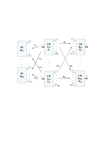
Figure 1: The system model for MIMO ad hoc CR networks.

Low-complexity receiver processing motivates the use of a linear filter matrix $\mathbf{W}_{k}\in\mathbb{C}^{M_{k}\times N_{k}}$ at $U_{k}^{r}$ to recover $\mathbf{s}_{k}$ as

$$\hat{\mathbf{s}}_{k}:=\mathbf{W}_{k}\mathbf{y}_{k},\quad k\in\mathcal{K}.$$ (2)

Using $\mathbf{W}_{k}$ at $U_{k}^{r}$, the MSE matrix $\mathbf{E}_{k}:=\mathbb{E}\{\left(\hat{\mathbf{s}}_{k}-\mathbf{s}_{k}\right)\left(\hat{\mathbf{s}}_{k}-\mathbf{s}_{k}\right)^{\cal H}\}$, which quantifies the reconstruction error, is given by [cf. (1)]

$$\mathbf{E}_{k}=\mathbf{W}_{k}\mathbf{A}_{k}\mathbf{W}^{{\cal H}}_{k}-\mathbf{W}_{k}\mathbf{H}_{k,k}\mathbf{F}_{k}-\mathbf{F}^{{\cal H}}_{k}\mathbf{H}^{{\cal H}}_{k,k}\mathbf{W}^{{\cal H}}_{k}+\mathbf{I}_{M_{k}}$$ (3)

where $\mathbf{A}_{k}:=\sum_{j=1}^{K}\mathbf{H}_{k,j}\mathbf{F}_{j}\mathbf{F}^{{\cal H}}_{j}\mathbf{H}^{{\cal H}}_{k,j}+\sigma_{k}^{2}\mathbf{I}_{N_{k}}$. Entry $(i,i)$ of $\mathbf{E}_{k}$ represents the MSE of the $i$-th data stream ($i$-th entry of $\mathbf{s}_{k}$) from $U_{k}^{t}$ to $U_{k}^{r}$, and $\textrm{Tr}\{\mathbf{E}_{k}\}$ corresponds to the MSE of $\hat{\mathbf{s}}_{k}$.

To complete the formulation, let $\mathbf{G}_{k}\in\mathbb{C}^{L\times M_{k}}$ denote the channel between CR $U_{k}^{t}$ and a PU receiver, possibly equipped with multiple ($L$) antennas, and $\iota^{\textrm{max}}$ the maximum instantaneous interference that the PU can tolerate. As in e.g., [11, 17], suppose that $\iota^{\textrm{max}}$ is pre-partitioned in per-CR transmitter portions $\{\iota_{k}^{\textrm{max}}\}$, possibly depending on QoS requirements of individual CR pairs. Then, the transmit- and receive-beamforming matrices minimizing the overall MSE can be obtained as (see also [6])

$$\textrm{(P1)}\quad\mathop{\textrm{min}}\limits_{\{\mathbf{F}_{k},\mathbf{W}_{k}\}^{K}_{k=1}} \sum^{K}_{k=1}\textrm{Tr}\{\mathbf{E}_{k}\}$$ (4a)

s. t. $$\textrm{Tr}\{\mathbf{F}_{k}\mathbf{F}^{{\cal H}}_{k}\}\leq p^{\textrm{max}}_{k},\,k\in{\cal K}~{}$$ (4b)

$$\textrm{Tr}\{\mathbf{G}_{k}\mathbf{F}_{k}\mathbf{F}^{{\cal H}}_{k}\mathbf{G}^{{\cal H}}_{k}\}\leq\iota_{k}^{\textrm{max}},\,k\in{\cal K}~{}$$ (4c)

where $p_{k}^{\textrm{max}}$ is the maximum transmit-power of $U_{k}^{t}$.

Remark 1 (Adopted performance metric). Among candidate performance metrics, the sum of MSEs from different data streams is adopted here, which has been widely employed in the beamforming literature; see e.g., [6, 7] and references therein. The relationships between MSE, bit error rate (BER) and SINR have been thoroughly considered in [22], and further investigated in [6]. Specifically, it has been shown that an improvement in the total MSE naturally translates in a lower BER. Furthermore, the sum of MSEs facilitates derivation of optimal filters, and the equivalence between minimizing the weighted sum of MSEs and maximizing the weighted sum rate has been established in [4, 23].

Unfortunately, due to lack of explicit cooperation between PU and CR nodes, CR-to-PU channels $\{\mathbf{G}_{k}\}$ are in general difficult to estimate accurately. As PU protection must be enforced though, it is important to take into account the CR-to-PU channel uncertainty, and guarantee that the interference power experienced by the PU receiver stays below a prescribed level for any possible (random) channel realization [12, 14]. Before developing a beamforming approach robust to inaccuracies associated with channel estimation, problem (P1) is conveniently re-formulated first in order to reduce the number of variables involved.

II-A Equivalent Optimization Problem

For the sum-MSE cost in (4a), the optimum $\{\mathbf{W}^{\textrm{opt}}_{k}\}$ will turn out to be expressible in closed form. To show this, note first that for fixed $\{\mathbf{F}_{k}\}$, (P1) is convex in $\mathbf{W}_{k}$, and $\{\mathbf{W}^{\textrm{opt}}_{k}\}$ can be obtained from the first-order optimality conditions. Express the Lagrangian function associated with (P1) as

$$\mathcal{L}\left({\cal P},{\cal D}\right)= \sum^{K}_{k=1}\textrm{Tr}\{\mathbf{E}_{k}\}+\sum^{K}_{k=1}\lambda_{k}\left(\textrm{Tr}\{\mathbf{F}_{k}\mathbf{F}^{{\cal H}}_{k}\}-p^{\textrm{max}}_{k}\right)$$

$$+\sum^{K}_{k=1}\nu_{k}\left(\textrm{Tr}\{\mathbf{G}_{k}\mathbf{F}_{k}\mathbf{F}^{{\cal H}}_{k}\mathbf{G}^{{\cal H}}_{k}\}-\iota_{k}^{\textrm{max}}\right)$$ (5)

where ${\cal P}:=\{\mathbf{F}_{k},\mathbf{W}_{k}\}_{k=1}^{K}$ and ${\cal D}:=\{\lambda_{k},\nu_{k}\}_{k=1}^{K}$ collects the primal and dual variables, respectively. Then, by equating the complex gradient $\partial\mathcal{L}\left({\cal P},{\cal D}\right)/\partial\mathbf{W}_{k}^{\ast}$ to zero, matrix $\mathbf{W}_{k}^{\textrm{opt}}$ is expressed as

$$\mathbf{W}^{\textrm{opt}}_{k}=\mathbf{F}^{{\cal H}}_{k}\mathbf{H}^{{\cal H}}_{k,k}\mathbf{A}_{k}^{-1},\quad k\in{\cal K}.$$ (6)

Clearly, the optimal set $\{\mathbf{W}^{\textrm{opt}}_{k}\}$ does not depend on channels $\{\mathbf{G}_{k}\}$, but only on $\{\mathbf{H}_{k,j}\}$.

Substituting $\{\mathbf{W}^{\textrm{opt}}_{k}\}$ into (4a), and using the covariance $\mathbf{Q}_{k}:=\mathbb{E}\{\mathbf{x}_{k}\mathbf{x}_{k}^{\cal H}\}=\mathbf{F}_{k}\mathbf{F}^{{\cal H}}_{k}$ as a matrix optimization variable, it follows that (P1) can be equivalently re-written as

$$\textrm{(P2)}\quad\mathop{\textrm{max}}\limits_{\{\mathbf{Q}_{k}\succeq\mathbf{0}\}} \sum^{K}_{k=1}u_{k}\left(\{\mathbf{Q}_{k}\}\right)$$ (7a)

s. t. $$\textrm{Tr}\{\mathbf{Q}_{k}\}\leq p^{\textrm{max}}_{k},\ k\in{\cal K}~{}$$ (7b)

$$\textrm{Tr}\{\mathbf{G}_{k}\mathbf{Q}_{k}\mathbf{G}^{{\cal H}}_{k}\}\leq\iota_{k}^{\textrm{max}},\ k\in{\cal K}~{}$$ (7c)

where the per-CR link utility $u_{k}\left(\{\mathbf{Q}_{k}\}\right)$ is given by

$$u_{k}\left(\{\mathbf{Q}_{k}\}\right) :=\textrm{Tr}\left\{\mathbf{H}_{k,k}\mathbf{Q}_{k}\mathbf{H}^{{\cal H}}_{k,k}\left(\mathbf{H}_{k,k}\mathbf{Q}_{k}\mathbf{H}^{{\cal H}}_{k,k}+\mathbf{R}_{k,k}\right)^{-1}\right\}$$ (8)

with $\mathbf{R}_{k,k}:=\sum_{i\neq k}\mathbf{H}_{k,i}\mathbf{Q}_{i}\mathbf{H}^{{\cal H}}_{k,i}+\sigma^{2}_{k}\mathbf{I}_{N_{k}}$. One remark is in order regarding (P2).

Remark 2 (Conventional MIMO networks). Upon discarding the interference constraints (7c), the beamforming problems formulated in this paper along with their centralized and distributed solvers can be considered also for non-CR MIMO ad-hoc and cellular networks in downlink or uplink operation.

Channels $\{\mathbf{G}_{k}\}$ must be perfectly known in order to solve (P2). A robust version of (P2), which accounts for imperfect channel knowledge, is dealt with in the next section.

II-B Robust Interference Constraint

In typical CR scenarios, CR-to-PU channels are challenging to estimate accurately. In fact, CR and PU nodes do not generally cooperate [1], thus rendering channel estimation challenging. To model estimation inaccuracies, consider expressing the CR-to-PU channel matrix $\mathbf{G}_{k}$ as

$$\mathbf{G}_{k}=\widehat{\mathbf{G}}_{k}+\Delta\mathbf{G}_{k}\,,\quad k\in{\cal K}$$ (9)

where $\widehat{\mathbf{G}}_{k}$ is the estimated channel, which is known at CR transmitter $U_{k}^{t}$, and $\{\Delta\mathbf{G}_{k}\}$ captures the underlying channel uncertainty [14, 16]. Specifically, the error matrix $\Delta\mathbf{G}_{k}$ is assumed to take values from the bounded set

$$\mathcal{G}_{k}:=\left\{\Delta\mathbf{G}_{k}|\textrm{Tr}\{\Delta\mathbf{G}_{k}\Delta\mathbf{G}_{k}^{{\cal H}}\}\leq\epsilon_{k}^{2}\right\},\,k\in{\cal K}$$ (10)

where $\epsilon_{k}>0$ specifies the radius of $\mathcal{G}_{k}$, and thus reflects the degree of uncertainty associated with $\widehat{\mathbf{G}}_{k}$. The set in (10) can be readily extended to the general ellipsoidal uncertainty model [18, Ch. 4]. Such an uncertainty model properly resembles the case where a time division duplex (TDD) strategy is adopted by the PU system, and CRs have prior knowledge of the PUs’ pilot sequence(s). But even without training symbols, CR-to-PU channel estimates can be formed using the deterministic path loss coefficients, and the size of the uncertainty region can be deduced from fading channel statistics. Compared to [12], the norm-bounded uncertainty model leads to worst-case interference constraints that ensure PU protection for any realization of the uncertain portion of the propagation channels.

Based on (10), a robust interference constraint can be written as

$$\textrm{Tr}\{(\widehat{\mathbf{G}}_{k}+\Delta\mathbf{G}_{k})\mathbf{Q}_{k}(\widehat{\mathbf{G}}_{k}+\Delta\mathbf{G}_{k})^{{\cal H}}\}\leq\iota_{k}^{\textrm{max}},$$

$$\forall~{}\Delta\mathbf{G}_{k}\in\mathcal{G}_{k},\,k\in{\cal K}$$ (11)

and consequently, a robust counterpart of (P2) can be formulated as follows

$$\textrm{(P3)}\quad\mathop{\textrm{max}}\limits_{\{\mathbf{Q}_{k}\succeq\mathbf{0}\}} \sum^{K}_{k=1}u_{k}\left(\{\mathbf{Q}_{k}\}\right)$$ (12a)

s. t. $$\textrm{Tr}\{\mathbf{Q}_{k}\}\leq p^{\textrm{max}}_{k},\ k\in{\cal K}~{}$$ (12b)

$$\textrm{Tr}\{\mathbf{G}_{k}\mathbf{Q}_{k}\mathbf{G}^{{\cal H}}_{k}\}\leq\iota_{k}^{\textrm{max}},\,\forall~{}\Delta\mathbf{G}_{k}\in\mathcal{G}_{k},\,k\in{\cal K}.~{}$$ (12c)

Clearly, once $\{\mathbf{Q}^{\textrm{opt}}_{k}\}$ are found by solving (P3), the wanted $\{\mathbf{W}^{\textrm{opt}}_{k}\}$ can be readily obtained via (6), since $\mathbf{A}_{k}:=\sum_{j=1}^{K}\mathbf{H}_{k,j}\mathbf{Q}_{j}\mathbf{H}^{{\cal H}}_{k,j}+\sigma_{k}^{2}\mathbf{I}_{N_{k}}$. However, $\sum_{k}u_{k}\left(\{\mathbf{Q}_{k}\}\right)$ is non-convex in $\{\mathbf{Q}_{k}\}$, and hence (P3) is hard to solve in general. Additionally, constraints (11) are not in a tractable form, which motivates their transformation. These issues are addressed in the next section. But first, two remarks are in order.

Remark 3 (Uncertain MIMO channels). In an underlay hierarchical spectrum access setup, it is very challenging (if not impossible) for the CRs to obtain accurate estimates of the CR-to-PU channels. In fact, since the PUs hold the spectrum license, they have no incentive to feed back CR-to-PU channel estimates to the CR system [1]. Hence, in lieu of explicit CR-PU cooperation, CRs have to resort to crude or blind estimates of their channels with PUs. On the other hand, sufficient time for training along with sophisticated estimation algorithms render the CR-to-CR channels easier to estimate. This explains why similar to relevant works [12, 13, 14, 15, 16, 17], CR-to-CR channels are assumed known, while CR-to-PU channels are taken as uncertain in CR-related optimization methods. Limited-rate channel state information that can become available e.g., with quantized CR-to-CR channels [6, 7, 12], can be considered in future research but goes beyond the scope of the present paper.

Remark 4 (Radius of the uncertainty region). In practice, radius and shape of the uncertainty region have to be tailored to the specific channel estimation approach implemented at the CRs, and clearly depend on the second-order channel error statistics. For example, if $\Delta\mathbf{G}_{k}$ has zero mean and covariance matrix $\mathbf{\Sigma}_{\Delta\mathbf{G}_{k}}=\hat{\sigma}^{2}_{k}\mathbf{I}$, where $\hat{\sigma}^{2}_{k}$ depends on the receiver noise power, and the transmit-power of the PU (see, e.g. [25]), then the radius of the uncertainty region can be set to $\epsilon_{k}^{2}=\kappa\xi_{k}\hat{\sigma}^{2}_{k}$, where $\xi_{k}$ denotes the path loss coefficient, and $\kappa>0$ a parameter that controls how strict the PU protection is. Alternatively, the model $\epsilon_{k}^{2}=\kappa\hat{\sigma}^{2}_{k}\|\hat{\mathbf{G}}_{k}\|_{F}^{2}$ can be utilized [17]. If $\mathbf{\Sigma}_{\Delta\mathbf{G}_{k}}\neq\hat{\sigma}^{2}_{k}\mathbf{I}$, then the uncertainty region can be set to $\mathcal{G}_{k}:=\left\{\Delta\mathbf{G}_{k}|\textrm{Tr}\{\Delta\mathbf{G}_{k}\mathbf{\Sigma}_{\Delta\mathbf{G}_{k}}^{-1}\Delta\mathbf{G}_{k}^{{\cal H}}\}\leq\kappa\right\}$ [24] and the robust constraint (11) can be modified accordingly. Similar models are also considered in [26].

III Distributed Robust CR Beamforming

To cope with the non-convexity of the utility function (12a), a block-coordinate ascent solver is developed in this section. Define first the sum of all but the $k$-th utility as $f_{k}(\mathbf{Q}_{k},\mathbf{Q}_{-k}):=\sum_{j\neq k}u_{j}$, with $\mathbf{Q}_{-k}:=\{\mathbf{Q}_{j}|j\neq k\}$. Notice that $u_{k}(\cdot)$ is concave and $f_{k}(\cdot)$ is convex in $\mathbf{Q}_{k}$; see Appendix -B for a proof. Then, (P3) can be regarded as a difference of convex functions (d.c.) program, whenever only a single variable $\mathbf{Q}_{k}$ is optimized and $\mathbf{Q}_{-k}$ is kept fixed. This motivates the so-termed concave-convex procedure [27], which belongs to the majorization-minimization class of algorithms [28], to solve problem (P3) through a sequence of convex problems, one per matrix variable $\mathbf{Q}_{k}$. Specifically, the idea is to linearize the convex function $f_{k}(\cdot)$ around a feasible point $\tilde{\mathbf{Q}}_{k}$, and thus to (locally) approximate the objective (12a) as (see also [5] and [10])

$$\sum^{K}_{k=1}u_{k}\left(\{\mathbf{Q}_{k}\}\right)=u_{k}\left(\{\mathbf{Q}_{k}\}\right)+f_{k}(\mathbf{Q}_{k},\mathbf{Q}_{-k})$$

$$\approx u_{k}\left(\{\mathbf{Q}_{k}\}\right)+f_{k}(\tilde{\mathbf{Q}}_{k},\mathbf{Q}_{-k})+\textrm{Tr}\left\{\mathbf{D}_{k}^{{\cal H}}(\mathbf{Q}_{k}-\tilde{\mathbf{Q}}_{k})\right\}$$ (13)

where

$$\mathbf{D}_{k}:=\nabla_{\mathbf{Q}_{k}}f_{k}(\tilde{\mathbf{Q}}_{k},\mathbf{Q}_{-k}):=\left.\frac{\partial f_{k}}{\partial\mathbf{Q}_{k}^{*}}\right|_{\mathbf{Q}_{k}=\tilde{\mathbf{Q}}_{k}}.$$ (14)

Therefore, for fixed $\mathbf{Q}_{-k}$, matrix $\mathbf{Q}_{k}$ can be obtained by solving the following sub-problem

$$\textrm{(P4)}\quad\mathop{\textrm{max}}\limits_{\mathbf{Q}_{k}}\quad u_{k}\left(\mathbf{Q}_{k},\mathbf{Q}_{-k}\right)+\textrm{Tr}\left\{\mathbf{D}_{k}^{{\cal H}}\mathbf{Q}_{k}\right\}~{}$$ (15a)

s. t. $$\mathbf{Q}_{k}\succeq\mathbf{0}$$ (15b)

$$\textrm{Tr}\{\mathbf{Q}_{k}\}\leq p^{\textrm{max}}_{k}$$ (15c)

$$\textrm{Tr}\{\mathbf{G}_{k}\mathbf{Q}_{k}\mathbf{G}^{{\cal H}}_{k}\}\leq\iota^{\textrm{max}}_{k},\ \forall~{}\Delta\mathbf{G}_{k}\in\mathcal{G}_{k}~{}$$ (15d)

where (see Appendix -A)

$$\mathbf{D}_{k} :=\left.-\sum_{j\neq k}\mathbf{H}^{{\cal H}}_{j,k}\mathbf{B}_{j}^{-1}\mathbf{V}_{j}\mathbf{B}_{j}^{-1}\mathbf{H}_{j,k}\right|_{\mathbf{Q}_{k}=\tilde{\mathbf{Q}}_{k}},~{}$$ (16)

$$\mathbf{B}_{j} :=\sum_{i=1}^{K}\mathbf{H}_{j,i}\mathbf{Q}_{i}\mathbf{H}^{{\cal H}}_{j,i}+\sigma^{2}_{j}\mathbf{I}_{N_{j}},$$ (17)

$$\mathbf{V}_{j} :=\mathbf{H}_{j,j}\mathbf{Q}_{j}\mathbf{H}_{j,j}^{{\cal H}}.$$ (18)

At each iteration $n=1,2,\ldots$, the block coordinate ascent solver amounts to updating the covariance matrices $\{\mathbf{Q}_{k}\}$ in a round robin fashion via (P4), where the solution obtained at the $(n-1)$-st iteration are exploited to compute the complex gradient (16). The term $\textrm{Tr}\left\{\mathbf{D}_{k}^{{\cal H}}\mathbf{Q}_{k}\right\}$ discourages a “selfish” behavior of the $k$-th CR-to-CR link, which would otherwise try to simply minimize its own MSE, as in the game-theoretic formulations of [11] and [17]. In the next subsection, the robust interference constraint will be translated to a tractable form, and (P4) will be re-stated accordingly.

III-A Equivalent robust interference constraint

Constraint (15d) renders (P4) a semi-infinite program (cf. [29, Ch. 3]). An equivalent constraint in linear matrix inequality (LMI) form will be derived next, thus turning (P4) into an equivalent semi-definite program (SDP), which can be efficiently solved in polynomial time by standard interior point methods. To this end, the following lemma is needed.

Lemma 1.

(S-Procedure [18, p. 655]) Consider $\mathbf{A},\mathbf{D}\in\mathbb{H}^{n\times n},\mathbf{b}\in\mathbb{C}^{n},c,e\in\mathbb{R}$, and assume the interior condition holds, i.e., there exists an $\bar{\mathbf{x}}$ satisfying $\bar{\mathbf{x}}^{{\cal H}}\mathbf{D}\bar{\mathbf{x}}<e$. Then, the inequality

$$\mathbf{x}^{{\cal H}}\mathbf{A}\mathbf{x}+2\Re(\mathbf{b}^{{\cal H}}\mathbf{x})+c\geq 0,~{}\forall~{}\mathbf{x}^{{\cal H}}\mathbf{D}\mathbf{x}\leq e$$ (19)

holds if and only if there exists $\theta\geq 0$ such that

$$\left[\begin{array}[]{cc}\theta\mathbf{D}+\mathbf{A}&\mathbf{b}\\ \mathbf{b}^{{\cal H}}&c-e\theta\end{array}\right]\succeq\mathbf{0}\,.$$ (22)

Using Lemma 1, the robust constraint (15d) can be equivalently reformulated as follows.

Proposition 1.

There exists $\theta_{k}\geq 0$, so that the robust interference constraint (15d) is equivalent to the following LMI

$$\left[\begin{array}[]{cc}\theta_{k}\mathbf{I}_{L\times M_{k}}-\left(\mathbf{I}_{L}\otimes\mathbf{Q}_{k}\right)&-\textnormal{{vec}}(\mathbf{Q}_{k}^{{\cal H}}\widehat{\mathbf{G}}_{k}^{{\cal H}})\\ -\textnormal{{vec}}(\mathbf{Q}_{k}^{{\cal H}}\widehat{\mathbf{G}}_{k}^{{\cal H}})^{{\cal H}}&\begin{array}[]{c}\iota^{\textrm{max}}_{k}-\epsilon_{k}^{2}\theta_{k}\\ -\textnormal{{Tr}}\{\widehat{\mathbf{G}}_{k}\mathbf{Q}_{k}\widehat{\mathbf{G}}^{{\cal H}}_{k}\}\end{array}\end{array}\right]\succeq\mathbf{0}\,.$$ (27)

Proof:

Using the properties of the trace operator $\textrm{Tr}(\mathbf{Z}^{{\cal H}}\mathbf{A}\mathbf{Z})=\textrm{vec}(\mathbf{Z})^{{\cal H}}(\mathbf{I}\otimes\mathbf{A})\textrm{vec}(\mathbf{Z})$ and $\textrm{Tr}(\mathbf{B}^{{\cal H}}\mathbf{Z})=\textrm{vec}(\mathbf{B})^{{\cal H}}\textrm{vec}(\mathbf{Z})$, constraint (15d) can be re-written as

$$~{}-\mathbf{g}_{k}^{{\cal H}}\left(\mathbf{I}_{L}\otimes\mathbf{Q}_{k}\right)\mathbf{g}_{k} -2\Re\left(\textrm{vec}(\mathbf{Q}_{k}^{{\cal H}}\widehat{\mathbf{G}}_{k}^{{\cal H}})^{{\cal H}}\mathbf{g}_{k}\right)$$

$$+\iota^{\textrm{max}}_{k}-\textrm{Tr}\{\widehat{\mathbf{G}}_{k}\mathbf{Q}_{k}\widehat{\mathbf{G}}^{{\cal H}}_{k}\}\geq 0,\,\forall~{}\|\mathbf{g}_{k}\|_{2}\leq\epsilon_{k}$$ (28)

where $\mathbf{g}_{k}:=\textrm{vec}(\Delta\mathbf{G}_{k}^{{\cal H}})$. Then, applying Lemma 1 to (III-A) yields readily (27). ∎

Proposition 2.

Problem (P4) can be equivalently re-written as the following SDP form:

$$\textnormal{(P5)}\quad\mathop{\textnormal{{min}}}_{\begin{subarray}{c}\mathbf{Q}_{k}\succeq\mathbf{0}\\ \mathbf{T},\theta_{k}\geq 0\end{subarray}}\quad \textnormal{{Tr}}\left\{\mathbf{T}\right\}-\textnormal{{Tr}}\left\{\mathbf{D}_{k}^{{\cal H}}\mathbf{Q}_{k}\right\}$$ (29a)

s. t. $$\textnormal{{Tr}}\{\mathbf{Q}_{k}\}\leq p^{\textrm{max}}_{k}$$ (29b)

$$\left[\begin{array}[]{cc}\mathbf{H}_{k,k}\mathbf{Q}_{k}\mathbf{H}^{{\cal H}}_{k,k}+\mathbf{R}_{k,k}&\mathbf{R}^{1/2}_{k,k}\\ \mathbf{R}^{1/2}_{k,k}&\mathbf{T}\end{array}\right]\succeq\mathbf{0}$$ (29e)

$$\left[\begin{array}[]{cc}\theta_{k}\mathbf{I}_{L\times M_{k}}-\left(\mathbf{I}_{L}\otimes\mathbf{Q}_{k}\right)&-\textnormal{{vec}}(\mathbf{Q}_{k}^{{\cal H}}\widehat{\mathbf{G}}_{k}^{{\cal H}})\\ -\textnormal{{vec}}(\mathbf{Q}_{k}^{{\cal H}}\widehat{\mathbf{G}}_{k}^{{\cal H}})^{{\cal H}}&\begin{array}[]{c}\iota^{\textrm{max}}_{k}-\epsilon_{k}^{2}\theta_{k}\\ -\textnormal{{Tr}}\{\widehat{\mathbf{G}}_{k}\mathbf{Q}_{k}\widehat{\mathbf{G}}^{{\cal H}}_{k}\}\end{array}\end{array}\right]\succeq\mathbf{0}\,.$$ (29j)

Proof:

First, note that [cf. (8)]

$$u_{k}\left(\mathbf{Q}_{k},\mathbf{Q}_{-k}\right)=\textrm{Tr}\left\{\mathbf{I}_{N_{k}}-\mathbf{R}_{k,k}\left(\mathbf{H}_{k,k}\mathbf{Q}_{k}\mathbf{H}^{{\cal H}}_{k,k}+\mathbf{R}_{k,k}\right)^{-1}\right\}.$$

Thus, (P4) is equivalent to

$$\mathop{\textrm{min}}_{\mathbf{Q}_{k}}\quad\textrm{Tr}\left\{\mathbf{R}_{k,k}^{1/2}\left(\mathbf{H}_{k,k}\mathbf{Q}_{k}\mathbf{H}^{{\cal H}}_{k,k}+\mathbf{R}_{k,k}\right)^{-1}\mathbf{R}_{k,k}^{1/2}\right\}$$

$$\hskip 128.0374pt-\textrm{Tr}\left\{\mathbf{D}_{k}^{{\cal H}}\mathbf{Q}_{k}\right\}$$

$$\textrm{s. t.}\quad\eqref{P5PSDCsrt}-\eqref{P5RobustInterf}.$$

Then, an auxiliary matrix variable $\mathbf{Y}$ is introduced such that $\mathbf{Y}\succeq\mathbf{R}_{k,k}^{1/2}\left(\mathbf{H}_{k,k}\mathbf{Q}_{k}\mathbf{H}^{{\cal H}}_{k,k}+\mathbf{R}_{k,k}\right)^{-1}\mathbf{R}_{k,k}^{1/2}$, which can be equivalently recast as (29e) by using the Schur complement [18]. Combining the LMI form of the robust interference constraint (27), the formulation of (P5) follows immediately. ∎

Problem (P3) can be solved in a centralized fashion upon collecting CR-to-CR channels $\{\mathbf{H}_{j,k}\}$, CR-to-PU estimated channels $\{\widehat{\mathbf{G}}_{k}\}$, and confidence intervals $\{\epsilon_{k}\}$ at a CR fusion center. The optimal transmit-covariance matrices can be found at the fusion center by solving (P5), and sent back to all CRs. This centralized scheme is tabulated as Algorithm 1, where $\mathbf{Q}_{k}^{(n)}$ denotes the transmit-covariance matrix of CR $U_{k}^{t}$ at iteration $n$ of the block coordinate ascent algorithm; $\mathbf{Q}^{(n)}:=\left(\mathbf{Q}_{1}^{(n)},\ldots,\mathbf{Q}_{K}^{(n)}\right)$ represents the set of transmit-covariance matrices at iteration $n$; ${\cal U}(\cdot)$ is the objective function (12a). A simple stopping criterion for terminating the iterations is ${\cal U}\left(\mathbf{Q}^{(n)}\right)-{\cal U}\left(\mathbf{Q}^{(n-1)}\right)<\upsilon$, where $\upsilon>0$ denotes a preselected threshold.

Algorithm 1 Centralized robust sum-MSE minimization

1:Collect all channel matrices $\{\mathbf{H}_{j,k}\}$, and noise powers $\{\sigma_{k}^{2}\}$

2:Collect all CR-to-PU channel matrices $\{\widehat{\mathbf{G}}_{k}\}$, and confidence intervals $\{\epsilon_{k}\}$

3:Initialize $\mathbf{Q}_{k}^{(0)}=\mathbf{0},\forall~{}k\in{\cal K}$

4:repeat ($n=1,2,\ldots$)

5:     for $k=1,2,\dots,K$ do

6:         Compute $\mathbf{D}_{k}^{(n)}$ via (16)

7:         Update $\mathbf{Q}_{k}^{(n)}$ by solving (P5) [(P6) for the proximal point-based method]

8:     end for

9:until ${\cal U}\left(\mathbf{Q}^{(n)}\right)-{\cal U}\left(\mathbf{Q}^{(n-1)}\right)<\upsilon$

10:Calculate $\{\mathbf{W}^{\textrm{opt}}_{k}\}$ via (6)

11:Broadcast optimal transmit- and receive-beamformers

To alleviate the high communication cost associated with the centralized setup, and ensure scalability with regards to network size and enhanced robustness to fusion center failure, a distributed optimization algorithm is generally desirable. It can be noticed that the proposed coordinate ascent approach lends itself to a distributed optimization procedure that can be implemented in an on-line fashion. Specifically, each CR $U_{k}^{t}$ can update locally $\mathbf{Q}_{k}$ via (P5) based on a measurement of the interference $\mathbf{R}_{k,k}^{(n)}$ [10], and the following information necessary to compute the complex gradient (16): i) its covariance matrix $\mathbf{Q}_{k}^{(n-1)}$ obtained at the previous iteration; ii) matrices $\{\mathbf{B}_{j}^{(n)}\}$ and $\{\mathbf{V}_{j}^{(n)}\}$ obtained from the neighboring CR links via local message passing. Furthermore, it is clear that the terms in (16) corresponding to CRs located far away from CR $U_{k}^{t}$ are negligible due to the path loss effect in channel $\{\mathbf{H}_{j,k}\}_{j\neq k}$; hence, summation in (16) is only limited to the interfering CRs, and consequently, matrices $\{\mathbf{B}_{j}^{(n)}\}$ and $\{\mathbf{V}_{j}^{(n)}\}$ need to be exchanged only locally. The overall distributed scheme is tabulated as Algorithm 2. The on-line implementation of the iterative optimization allows tracking of slow variations of the channel matrices; in this case, cross-channels $\{\mathbf{H}_{j,k}\}$ in Algorithm 2 need to be re-acquired whenever a change is detected. Finally, notice that instead of updating the transmit-covariances in a Gauss-Seidel fashion, Jacobi iterations or asynchronous schemes [19] can be alternatively employed.

Algorithm 2 Distributed on-line robust sum-MSE minimization

1:Initialize $\mathbf{Q}_{k}^{(0)}=\mathbf{0},\forall~{}k\in{\cal K}$

2:repeat ($n=1,2,\ldots$)

3:     for $k=1,2,\dots,K$ do

4:         $U_{k}^{t}$ acquires $\mathbf{H}_{j,k}$ from its neighboring $U_{j}^{r}$

5:         transmit $\{\mathbf{B}_{k}^{(n)},\mathbf{V}_{k}^{(n)}\}$ to neighboring nodes

6:         receive $\{\mathbf{B}_{j}^{(n)},\mathbf{V}_{j}^{(n)}\}_{j\neq k}$ from neighboring nodes

7:         Compute $\mathbf{D}_{k}^{(n)}$ via (16)

8:         Measure $\mathbf{R}_{k,k}^{(n)}$

9:         Update $\mathbf{Q}_{k}^{(n)}$ by solving (P5) [(P6) for the proximal point-based method]

10:         Update $\mathbf{W}_{k}^{(n)}$ via (6)

11:         Transmit and receive signals using $\mathbf{Q}_{k}^{(n)}$ and $\mathbf{W}_{k}^{(n)}$

12:     end for

13:until $u_{k}\left(\mathbf{Q}^{(n)}\right)-u_{k}\left(\mathbf{Q}^{(n-1)}\right)<\upsilon$, $\forall~{}k\in{\cal K}$

Remark 5 (Multiple PU receivers). For ease of exposition, the formulated robust optimization problems consider a single PU receiver. Clearly, in case of $N_{\textrm{PU}}>1$ receiving PU devices, or when a grid of $N_{\textrm{PU}}$ potential PU locations is obtained from the sensing phase [30], a robust interference constraint for each of the $KN_{\textrm{PU}}$ CR-to-PU links must be included in (P3). As for (P5), it is still an SDP, but with $N_{\textrm{PU}}$ LMI constraints (29j), and one additional optimization variable ($\theta_{k}$) per PU receiver.

Remark 6 (Network synchronization). Similar to [6, 4, 5, 7, 13, 8, 9, 10, 11, 17, 14, 22, 15, 16, 23, 24], time synchronization is assumed to have been acquired. In practice, accurate time synchronization among the CR transmitters can be attained (and maintained during operation) using e.g., pairwise broadcast synchronization protocols [31], consensus-based methods [32], or mutual network synchronization approaches [33]. To this end, CRs have to exchange synchronization beacons on a regular basis; clearly, the number of time slots occupied by the transmission of these beacons depends on the particular algorithm implemented, the CR network size, and the targeted synchronization accuracy. For example, the algorithm in [31] entails two message exchanges per transmitter pairs, while the message-passing overhead of consensus-based methods generally depends on the wanted synchronization accuracy [32]. Since the CR network operates in an underlay setup, this additional message passing can be performed over the primary channel(s). Alternatively, a CR control channel can be employed to avoid possible synchronization errors due to the interference inflicted by the active PU transmitters. Analyzing the effect of mistiming constitutes an interesting research direction, but it goes beyond the scope and page limit of this paper.

III-B Convergence

Since the original optimization problem (P3) is non-convex, convergence of the block coordinate ascent with local convex approximation has to be analytically established. To this end, recall that (P4) and (P5) are equivalent; thus, convergence can be asserted by supposing that (P4) is solved per Gauss-Seidel iteration instead of (P5). The following lemma (proved in Appendix -B) is needed first.

Lemma 2.

For each $k\in{\cal K}$, the feasible set of problem (P4), namely $\mathcal{Q}_{k}:=\{\mathbf{Q}_{k}|\mathbf{Q}_{k}\in(\ref{P5PSDCsrt})-(\ref{P5RobustInterf})\}$, is convex. The real-valued function $f_{k}(\mathbf{Q}_{k},\mathbf{Q}_{-k})$ is convex in $\mathbf{Q}_{k}$ over the feasible set $\mathcal{Q}_{k}$, when the set $\mathbf{Q}_{-k}:=\{\mathbf{Q}_{j},j\neq k\}$ is fixed.

Based on Lemma 2, convergence of the block coordinate ascent algorithm is established next.

Proposition 3.

The sequence of objective function values (12a) obtained by the coordinate ascent algorithm with concave-convex procedure converges.

Proof:

It suffices to show that the sequence of objective values (12a) is monotonically non-decreasing. Since the objective function value is bounded from above, the function value sequence must be convergent by invoking the monotone convergence theorem. Letting $\widetilde{{\cal U}}_{k}(\cdot)$ denote the objective function (15a), which is the concave surrogate of ${\cal U}(\cdot)$ as the original objective (12a), consider

$$\mathbf{Q}_{k}^{(n)}:=$$

$$\operatorname*{arg\,max}_{\mathbf{Q}_{k}\in{\cal Q}_{k}}\,\,\widetilde{{\cal U}}_{k}\left(\mathbf{Q}_{k};\mathbf{Q}_{1}^{(n)},\ldots,\mathbf{Q}_{k-1}^{(n)},\mathbf{Q}_{k+1}^{(n-1)},\ldots,\mathbf{Q}_{K}^{(n-1)}\right)$$ (30)

where $n$ stands for the iteration index. Furthermore, define

$$\mathbf{Z}_{k}^{(n)} :=(\mathbf{Q}_{1}^{(n+1)},\ldots,\mathbf{Q}_{k}^{(n+1)},\mathbf{Q}_{k+1}^{(n)},\ldots,\mathbf{Q}_{K}^{(n)}),$$ (31)

$$\tilde{\mathbf{Q}}^{(n)}_{-k} :=(\mathbf{Q}_{1}^{(n+1)},\ldots,\mathbf{Q}_{k-1}^{(n+1)},\mathbf{Q}_{k+1}^{(n)},\ldots,\mathbf{Q}_{K}^{(n)}).~{}$$ (32)

Then, for all $k\in{\cal K}$, it holds that

$${\cal U}\left(\mathbf{Z}_{k}^{(n)}\right) =u_{k}\left(\mathbf{Q}_{k}^{(n+1)},\tilde{\mathbf{Q}}^{(n)}_{-k}\right)+f_{k}\left(\mathbf{Q}_{k}^{(n+1)},\tilde{\mathbf{Q}}^{(n)}_{-k}\right)$$ (33a)

$$\geq u_{k}\left(\mathbf{Q}_{k}^{(n+1)},\tilde{\mathbf{Q}}^{(n)}_{-k}\right)+f_{k}\left(\mathbf{Q}_{k}^{(n)},\tilde{\mathbf{Q}}^{(n)}_{-k}\right)$$

$$\hskip 45.52458pt+\textrm{Tr}\left\{\mathbf{D}^{{\cal H}}_{k}\left(\mathbf{Q}_{k}^{(n+1)}-\mathbf{Q}_{k}^{(n)}\right)\right\}$$ (33b)

$$\geq u_{k}\left(\mathbf{Q}_{k}^{(n)},\tilde{\mathbf{Q}}^{(n)}_{-k}\right)+f_{k}\left(\mathbf{Q}_{k}^{(n)},\tilde{\mathbf{Q}}^{(n)}_{-k}\right)$$

$$\hskip 45.52458pt+\textrm{Tr}\left\{\mathbf{D}^{{\cal H}}_{k}\left(\mathbf{Q}_{k}^{(n)}-\mathbf{Q}_{k}^{(n)}\right)\right\}$$ (33c)

$$={\cal U}\left(\mathbf{Z}_{k-1}^{(n)}\right)$$ (33d)

where (33b) follows from the convexity of $f_{k}(\cdot)$ established in Lemma 2;  (33c) holds because $\mathbf{Q}_{k}^{(n+1)}$ is the optimal solution of (P4) for fixed $\tilde{\mathbf{Q}}^{(n)}_{-k}$.

To complete the proof, it suffices to show that ${\cal U}\left(\mathbf{Q}^{(n+1)}\right)$ is monotonically non-decreasing, namely that

$${\cal U}\left(\mathbf{Q}^{(n+1)}\right)\geq{\cal U}\left(\mathbf{Z}_{K-1}^{(n)}\right)\geq\ldots\geq{\cal U}\left(\mathbf{Z}_{1}^{(n)}\right)\geq{\cal U}\left(\mathbf{Q}^{(n)}\right)$$ (34)

∎

Interestingly, by inspecting the structure of $\{\mathbf{H}_{k,k},k\in{\cal K}\}$, it is also possible to show that every limit point generated by the coordinate ascent algorithm with local convex approximation satisfies the first-order optimality conditions. Conditions on $\{\mathbf{H}_{k,k},k\in{\cal K}\}$ that guarantee stationarity of the limit points are provided next. First, it is useful to establish strict concavity of the objective (15a) in the following lemma proved in Appendix -C.

Lemma 3.

If the channel matrices $\{\mathbf{H}_{k,k},k\in{\cal K}\}$ of the CR links $\{U_{k}^{t}\rightarrow U_{k}^{r}\}$ have full column rank, then the objective function (15a) is strictly concave in $\mathbf{Q}_{k}$.

We are now ready to establish stationarity of the limit points.

Theorem 1.

If matrices $\{\mathbf{H}_{k,k},k\in{\cal K}\}$ have full column rank, then every limit point of the coordinate ascent algorithm with concave-convex procedure is a stationary point of (P3).

Proof:

The proof of Theorem 1 relies on the basic convergence claim of the block coordinate descent method in [29, Ch. 2] and [5]. What must be shown is that every limit point of the algorithm satisfies the first-order optimality conditions over the Cartesian product of the closed convex sets. Let $\bar{\mathbf{Q}}:=\left(\bar{\mathbf{Q}}_{1},\ldots,\bar{\mathbf{Q}}_{K}\right)$ be a limit point of the sequence $\{\mathbf{Q}^{(n)}\}$, and $\{\mathbf{Q}^{(n_{j})}|j=1,2,\ldots\}$ a subsequence that converges to $\bar{\mathbf{Q}}$. First, we will show that $\lim\limits_{j\rightarrow\infty}\mathbf{Q}_{1}^{(n_{j}+1)}=\bar{\mathbf{Q}}_{1}$. Argue by contradiction, i.e., assume that $\{\mathbf{Q}_{1}^{(n_{j}+1)}-\mathbf{Q}_{1}^{(n_{j})}\}$ does not converge to zero. Define $\gamma^{(n_{j})}:=\|\mathbf{Q}_{1}^{(n_{j}+1)}-\mathbf{Q}_{1}^{(n_{j})}\|_{F}$. By possibly restricting to a subsequence of $\{n_{j}\}$, it follows that there exists some $\bar{\gamma}>0$ such that $\bar{\gamma}\leq\gamma^{(n_{j})}$ for all $j$. Let $\mathbf{S}_{1}^{(n_{j})}:=(\mathbf{Q}_{1}^{(n_{j}+1)}-\mathbf{Q}_{1}^{(n_{j})})/\gamma^{(n_{j})}$. Thus, we have that $\mathbf{Q}_{1}^{(n_{j}+1)}=\mathbf{Q}_{1}^{(n_{j})}+\gamma^{(n_{j})}\mathbf{S}_{1}^{(n_{j})}$ and $\|\mathbf{S}_{1}^{(n_{j})}\|_{F}=1$. Because $\mathbf{S}_{1}^{(n_{j})}$ belongs to a compact set, it can be assumed convergent to a limit point $\bar{\mathbf{S}}_{1}$ along with a subsequence of $\{n_{j}\}$.

Since it holds that $0\leq\epsilon\bar{\gamma}\leq\gamma^{(n_{j})}$ for all $\epsilon\in[0,1]$, the point $\mathbf{Q}_{1}^{(n_{j})}+\epsilon\bar{\gamma}\mathbf{S}_{1}^{(n_{j})}$ lies on the segment connecting two feasible points $\mathbf{Q}_{1}^{(n_{j})}$ and $\mathbf{Q}_{1}^{(n_{j}+1)}$. Thus, $\mathbf{Q}_{1}^{(n_{j})}+\epsilon\bar{\gamma}\mathbf{S}_{1}^{(n_{j})}$ is also feasible due to the convexity of ${\cal Q}_{1}$ [cf. Lemma 2]. Moreover, concavity of $\widetilde{{\cal U}}_{1}(\cdot;\mathbf{Q}_{-1}^{(n_{j})})$ implies that $\widetilde{{\cal U}}_{1}$ is monotonically non-decreasing in the interval connecting point $\mathbf{Q}_{1}^{(n_{j})}$ to $\mathbf{Q}_{1}^{(n_{j}+1)}$ over the set ${\cal Q}_{1}$. Hence, it readily follows that

$$\widetilde{{\cal U}}_{1}(\mathbf{Q}_{1}^{(n_{j}+1)};\mathbf{Q}_{-1}^{(n_{j})})\geq\widetilde{{\cal U}}_{1}(\mathbf{Q}_{1}^{(n_{j})}+\epsilon\bar{\gamma}\mathbf{S}_{1}^{(n_{j})};\mathbf{Q}_{-1}^{(n_{j})})$$

$$\geq\widetilde{{\cal U}}_{1}(\mathbf{Q}_{1}^{(n_{j})};\mathbf{Q}_{-1}^{(n_{j})}).~{}$$ (35)

Note that $\widetilde{{\cal U}}_{1}(\cdot)$ is a tight lower bound of ${\cal U}(\cdot)$ at each current feasible point. Also, from (34), $\widetilde{{\cal U}}_{1}(\mathbf{Q}_{1}^{(n_{j}+1)};\mathbf{Q}_{-1}^{(n_{j})})$ is guaranteed to converge to $\widetilde{{\cal U}}_{1}(\bar{\mathbf{Q}})$ as $j\rightarrow\infty$. Thus, upon taking the limit as $j\rightarrow\infty$ in (35), it follows that

$$\widetilde{{\cal U}}_{1}(\bar{\mathbf{Q}}_{1}+\epsilon\bar{\gamma}\bar{\mathbf{S}}_{1};\bar{\mathbf{Q}}_{-1})=\widetilde{{\cal U}}_{1}(\bar{\mathbf{Q}}),\quad\forall~{}\epsilon\in[0,1]\,.~{}$$ (36)

However, since $\bar{\gamma}\bar{\mathbf{S}}_{1}\neq\mathbf{0}$, (36) contradicts the unique maximum condition implied by the strict concavity of $\widetilde{{\cal U}}_{1}(\cdot;\cdot)$ in $\mathbf{Q}_{1}$ [cf. Lemma 3]. Therefore, $\mathbf{Q}_{1}^{(n_{j}+1)}$ converges to $\bar{\mathbf{Q}}_{1}$ as well.

Consider now checking the optimality condition for $\bar{\mathbf{Q}}_{1}$. Since $\mathbf{Q}_{1}^{(n_{j}+1)}$ is the local (and also global) maximum of $\widetilde{{\cal U}}_{1}(\cdot;\mathbf{Q}_{-1}^{(n_{j})})$, we have that

$$\Re\left\{\textrm{Tr}\left\{\nabla_{1}\widetilde{{\cal U}}_{1}\left(\mathbf{Q}_{1}^{(n_{j}+1)};\mathbf{Q}_{-1}^{(n_{j})}\right)^{{\cal H}}\left(\mathbf{Q}_{1}-\mathbf{Q}_{1}^{(n_{j}+1)}\right)\right\}\right\} \leq 0,$$

$$\forall~{}\mathbf{Q}_{1}\in{\cal Q}_{1}~{}$$ (37)

where $\nabla_{1}\widetilde{{\cal U}}_{1}(\cdot)$ denotes the gradient of $\widetilde{{\cal U}}_{1}(\cdot)$ with respect to $\mathbf{Q}_{1}$. Taking the limit as $j\rightarrow\infty$, and using the fact that $\nabla_{1}\widetilde{{\cal U}}_{1}(\bar{\mathbf{Q}})=\nabla_{1}{\cal U}_{1}(\bar{\mathbf{Q}})$, it is easy to show that

$$\Re\left\{\textrm{Tr}\left\{\nabla_{1}{{\cal U}}(\bar{\mathbf{Q}})^{{\cal H}}(\mathbf{Q}_{1}-\bar{\mathbf{Q}}_{1})\right\}\right\}\leq 0,\quad\forall~{}\mathbf{Q}_{1}\in{\cal Q}_{1}.~{}$$ (38)

Using similar arguments, it holds that

$$\Re\left\{\textrm{Tr}\left\{\nabla_{i}{{\cal U}}(\bar{\mathbf{Q}})^{{\cal H}}(\mathbf{Q}_{i}-\bar{\mathbf{Q}}_{i})\right\}\right\} \leq 0,$$

$$\forall~{}\mathbf{Q}_{i}\in{\cal Q}_{i},~{}i=1,2,\ldots,K~{}$$ (39)

which establishes the stationarity of $\bar{\mathbf{Q}}$ and completes the proof. ∎

III-C Proximal point-based robust algorithm

The full column rank requirement can be quite restrictive in practice; e.g., if $M_{k}>N_{k}$ for at least one CR link, or in the presence of spatially correlated MIMO channels [20]. Furthermore, computing the rank of channel matrices increases the computational burden to an extent that may not be affordable by the CRs. In this section, an alternative approach based on proximal-point regularization [21] is pursued to ensure convergence, without requiring restrictions on the antenna configuration and the channel rank.

The idea consists in penalizing the objective of (P4) using a quadratic regularization term $\frac{1}{2\tau_{k}}\|\mathbf{Q}_{k}-\mathbf{Q}_{k}^{(n-1)}\|^{2}_{F}$, with a given sequence of numbers $\tau_{k}>0$. Then, (P5) is modified as

$$\text{(P6)}\,\,\mathop{\textrm{min}}_{\begin{subarray}{c}\mathbf{Q}_{k}\succeq\mathbf{0},\theta_{k}\geq 0\\ \mathbf{T},\mathbf{Y}\end{subarray}}\, \textrm{Tr}\left\{\mathbf{T}\right\}-\textrm{Tr}\left\{\mathbf{D}_{k}^{{\cal H}}\mathbf{Q}_{k}\right\}+\frac{1}{2\tau_{k}}\textrm{Tr}\{\mathbf{Y}\}$$ (40a)

s. t. $$\left[\begin{array}[]{cc}\mathbf{I}_{M_{k}}&\mathbf{Q}_{k}-\mathbf{Q}_{k}^{(n-1)}\\ \mathbf{Q}_{k}-\mathbf{Q}_{k}^{(n-1)}&\mathbf{Y}\end{array}\right]\succeq\mathbf{0}$$ (40d)

$$\,\,\eqref{P6TxPower},\eqref{P6SchurSDP},\eqref{P6RobustInterf}$$

where (40d) is derived by using the Schur complement through the auxiliary variable $\mathbf{Y}$.

The role of $\frac{1}{2\tau_{k}}\|\mathbf{Q}_{k}-\mathbf{Q}_{k}^{(n-1)}\|^{2}_{F}$ is to render the cost in (40a) strictly convex and coercive. Moreover, for small values of $\tau_{k}$, the optimization variable $\mathbf{Q}_{k}$ is forced to stay “close” to $\mathbf{Q}_{k}^{(n-1)}$ obtained at the previous iteration, thereby improving the stability of the iterates [34, Ch. 6]. Centralized and distributed schemes with the proximal point regularization are given by Algorithms 1 and 2, respectively, with problem (P6) replacing (P5). Convergence of the resulting schemes is established in the following theorem. To avoid ambiguity, these proximal point-based algorithms will be hereafter referred as Algorithms 1(P) and 2(P), respectively.

Theorem 2.

Suppose that the sequence $\{\mathbf{Q}^{(n)}\}$ generated by Algorithm 1(P) (Algorithm 2(P)) has a limit point. Then, every limit point is a stationary point of (P3).

Proof:

The Gauss-Seidel method with a proximal point regularization converges without any underlying convexity assumptions [35]. A modified version of the proof is reported here, where the local convex approximation (13) and the peculiarities of the problem at hand are leveraged to establish not only convergence of the algorithm, but also optimality of the obtained solution.

Assume there exists a subsequence $\{\mathbf{Q}^{(n_{j})}|j=1,2,\ldots\}$ converging to a limit point $\bar{\mathbf{Q}}:=\left(\bar{\mathbf{Q}}_{1},\ldots,\bar{\mathbf{Q}}_{K}\right)$. Let $\mathbf{Q}_{k}^{(n+1)}$ be obtained as

$$\mathbf{Q}_{k}^{(n+1)}:=$$

$$\operatorname*{arg\,max}_{\mathbf{Q}_{k}\in{\cal Q}_{k}}\,\,\widetilde{{\cal U}}_{k}\left(\mathbf{Q}_{k};\mathbf{Q}_{1}^{(n+1)},\ldots,\mathbf{Q}_{k-1}^{(n+1)},\mathbf{Q}_{k+1}^{(n)},\ldots,\mathbf{Q}_{K}^{(n)}\right)$$

$$\hskip 128.0374pt-\frac{1}{2\tau_{k}}\|\mathbf{Q}_{k}-\mathbf{Q}^{(n)}_{k}\|^{2}_{F}\,.$$ (41)

Thus, it follows that [cf. (32)]

$$\widetilde{{\cal U}}_{1}(\mathbf{Q}_{1}^{(n_{j}+1)};\tilde{\mathbf{Q}}_{-1}^{(n_{j})}) \geq\widetilde{{\cal U}}_{1}(\mathbf{Q}_{1}^{(n_{j})};\tilde{\mathbf{Q}}_{-1}^{(n_{j})})$$

$$\hskip 19.91684pt+\frac{1}{2\tau_{k}}\|\mathbf{Q}_{1}^{(n_{j}+1)}-\mathbf{Q}_{1}^{(n_{j})}\|^{2}_{F}\,.$$ (42)

Going along the lines of the proof of Theorem 1, it holds that

$$\lim\limits_{j\rightarrow\infty}\widetilde{{\cal U}}_{1}(\mathbf{Q}_{1}^{(n_{j}+1)};\tilde{\mathbf{Q}}_{-1}^{(n_{j})})=\lim\limits_{j\rightarrow\infty}\widetilde{{\cal U}}_{1}(\mathbf{Q}_{1}^{(n_{j})};\tilde{\mathbf{Q}}_{-1}^{(n_{j})})=\widetilde{{\cal U}}_{1}(\bar{\mathbf{Q}}).~{}$$ (43)

Therefore, taking the limit as $j\rightarrow\infty$ in (42), one arrives at

$$\lim\limits_{j\rightarrow\infty}\|\mathbf{Q}_{1}^{(n_{j}+1)}-\mathbf{Q}_{1}^{(n_{j})}\|_{F}^{2}=0$$ (44)

which implies that $\mathbf{Q}_{1}^{(n_{j}+1)}$ also converges to $\bar{\mathbf{Q}}_{1}$.

Since $\mathbf{Q}_{1}^{(n_{j}+1)}$ is generated as in (41), it satisfies the optimality condition

$$\Re\Bigg{\{} \textrm{Tr}\Bigg{\{}\left[\nabla_{1}\widetilde{{\cal U}}_{1}(\mathbf{Q}_{1}^{(n_{j}+1)};\mathbf{Q}_{-1}^{(n_{j})})-\frac{1}{\tau_{1}}(\mathbf{Q}_{1}^{(n_{j}+1)}-\mathbf{Q}_{1}^{(n_{j})})\right]^{{\cal H}}$$

$$\hskip 39.83368pt(\mathbf{Q}_{1}-\mathbf{Q}_{1}^{(n_{j}+1)})\Bigg{\}}\Bigg{\}}\leq 0,\quad\forall~{}\mathbf{Q}_{1}\in{\cal Q}_{1}.~{}$$ (45)

Taking the limit as $j\rightarrow\infty$ in (45), and using again the fact that $\nabla_{1}\widetilde{{\cal U}}_{1}(\bar{\mathbf{Q}})=\nabla_{1}{\cal U}_{1}(\bar{\mathbf{Q}})$, we obtain

$$\Re\left\{\textrm{Tr}\left\{\nabla_{1}{{\cal U}}(\bar{\mathbf{Q}})^{{\cal H}}(\mathbf{Q}_{1}-\bar{\mathbf{Q}}_{1})\right\}\right\}\leq 0,\quad\forall~{}\mathbf{Q}_{1}\in{\cal Q}_{1}\,.$$ (46)

Then, repeating the same argument for all $k\in{\cal K}$, leads to

$$\Re\left\{\textrm{Tr}\left\{\nabla_{k}{{\cal U}}(\bar{\mathbf{Q}})^{{\cal H}}(\mathbf{Q}_{k}-\bar{\mathbf{Q}}_{k})\right\}\right\}\leq 0,\quad\forall~{}\mathbf{Q}_{k}\in{\cal Q}_{k}~{}$$ (47)

which shows that the limit point $\bar{\mathbf{Q}}$ is also a stationary point. ∎

As asserted in Theorem 2, Algorithms 1(P) and 2(P) converge to a stationary point of (P3) for any possible antenna configuration. The price to pay however, is a possibly slower convergence rate that is common to proximal point-based methods [34, Ch. 6] (see also the numerical tests in Section V). For this reason, the proximal point-based method should be used in either a centralized or a distributed setup whenever the number of transmit-antennas exceeds that of receive-antennas in at least one transmitter-receiver pair. In this case, Algorithms 1(P) and 2(P) ensure first-order optimality of the solution obtained. When $M_{k}\leq N_{k}$, for all $k\in{\cal K}$, the two solvers have complementary strengths in convergence rate and computational complexity. Specifically, Algorithms 1 and 2 require the rank of all CR direct channel matrices $\{\mathbf{H}_{k,k}\}$ beforehand, which can be computationally burdensome, especially for a high number of antenna elements. If the rank determination can be afforded, and the convergence rate is at a premium, then Algorithms 1 and 2 should be utilized.

IV Aggregate Interference Constraints

Suppose now that the individual interference budgets $\{\iota_{k}^{\textrm{max}}\}$ are not available a priori. Then, the aggregate interference power $\{\iota^{\textrm{max}}\}$ has to be divided among transmit-CRs by the resource allocation scheme in order for the overall system performance to be optimized. Accordingly, (P3) is modified as follows to incorporate a robust constraint on the total interference power inflicted to the PU node:

$$\textrm{(P7)}\quad\mathop{\textrm{max}}\limits_{\{\mathbf{Q}_{k}\}^{K}_{k=1}} \sum^{K}_{k=1}u_{k}(\{\mathbf{Q}_{k}\})$$ (48a)

s. t. $$\textrm{Tr}\{\mathbf{Q}_{k}\}\leq p^{\textrm{max}}_{k},\,k\in{\cal K}$$ (48b)

$$\sum_{k=1}^{K}\textrm{Tr}\{\mathbf{G}_{k}\mathbf{Q}_{k}\mathbf{G}^{{\cal H}}_{k}\}\leq\iota^{\textrm{max}},\,\forall~{}\Delta\mathbf{G}_{k}\in\mathcal{G}_{k},\,k\in{\cal K}.$$ (48c)

The new interference constraint (48c) couples the CR nodes (or, more precisely, the subset of transmit-CR nodes in the proximity of the PU receiver). Thus, the overhead of message passing increases since cooperation among coupled CR nodes is needed.

A common technique for dealing with coupled constraints is the dual decomposition method [29], which facilitates evaluation of the dual function by dualizing the coupled constraints. However, since (P7) is non-convex and non-separable, the duality gap is generally non-zero. Thus, the primal variables obtained during the intermediate iterates may not be feasible, i.e., transmit-covariances can possibly lead to violation of the interference constraint. Since the ultimate goal is to design an on-line algorithm where (48c) must be satisfied during network operation, the primal decomposition technique is well motivated to cope with the coupled interference constraints [10]. To this end, consider introducing two sets of auxiliary variables $\{\iota_{k}\}$ and $\{t_{k}\}$ in problem (P7), which is equivalently re-formulated as

(P8)

$$\mathop{\textrm{max}}\limits_{\{\mathbf{Q}_{k},\iota_{k},t_{k}\}} \sum^{K}_{k=1}\textrm{Tr}\left\{\mathbf{H}_{k,k}\mathbf{Q}_{k}\mathbf{H}^{{\cal H}}_{k,k}\left(\mathbf{H}_{k,k}\mathbf{Q}_{k}\mathbf{H}^{{\cal H}}_{k,k}+\mathbf{R}_{k,k}\right)^{-1}\right\}$$ (49a)

s. t. $$\textrm{Tr}\{\mathbf{Q}_{k}\}\leq p^{\textrm{max}}_{k},\quad k\in{\cal K}~{}$$ (49b)

$$\textrm{Tr}\{\mathbf{G}_{k}\mathbf{Q}_{k}\mathbf{G}^{{\cal H}}_{k}\}\leq t_{k},~{}\forall~{}\Delta\mathbf{G}_{k}\in\mathcal{G}_{k},k\in{\cal K}~{}$$ (49c)

$$0\leq t_{k}\leq\iota_{k},\quad k\in{\cal K}$$ (49d)

$$\sum_{k=1}^{K}\iota_{k}\leq\iota^{\textrm{max}}\,.$$ (49e)

For fixed $\{\iota_{k}\}$, the inner maximization subproblem turns out to be

$$\textrm{(P9)}\quad p( \{\iota_{k}\}):=$$

$$\mathop{\textrm{max}}\limits_{\{\mathbf{Q}_{k},t_{k}\}} \sum^{K}_{k=1}\textrm{Tr}\left\{\mathbf{H}_{k,k}\mathbf{Q}_{k}\mathbf{H}^{{\cal H}}_{k,k}\left(\mathbf{H}_{k,k}\mathbf{Q}_{k}\mathbf{H}^{{\cal H}}_{k,k}+\mathbf{R}_{k,k}\right)^{-1}\right\}$$ (50a)

s. t. $$\textrm{Tr}\{\mathbf{Q}_{k}\}\leq p^{\textrm{max}}_{k},\quad k\in{\cal K}~{}$$ (50b)

$$\textrm{Tr}\{\mathbf{G}_{k}\mathbf{Q}_{k}\mathbf{G}^{{\cal H}}_{k}\}\leq t_{k},~{}\forall~{}\Delta\mathbf{G}_{k}\in\mathcal{G}_{k},k\in{\cal K}~{}$$ (50c)

$$0\leq t_{k}\leq\iota_{k},\quad k\in{\cal K}$$ (50d)

which, as discussed in preceding sections, can be solved using the block coordinate ascent algorithm (or its proximal point version) in either a centralized or a distributed fashion. After solving (P9) for a given set $\{\iota_{k}\}$, the per-CR interference budgets $\{\iota_{k}\}$ are updated by the following master problem:

$$\textrm{(P10)}\quad\mathop{\textrm{max}}_{\{\iota_{k}\}}~{} p(\{\iota_{k}\})$$ (51a)

s. t. $$\{\iota_{k}\}\in\mathcal{I}$$ (51b)

with the simplex set $\mathcal{I}$ given by

$$\mathcal{I}:=\left\{\{\iota_{k}\}|\iota_{k}\geq 0,\sum^{K}_{k=1}\iota_{k}\leq\iota^{\textrm{max}}\right\}\,.$$ (52)

Overall, the primal decomposition method solves (P8) by iteratively solving (P9) and (P10). Notice that the master problem (P10) dynamically divides the total interference budget $\iota^{\textrm{max}}$ among CR transmitters, so as to find the best allocation of resources that maximizes the overall system performance. Using the block coordinate ascent algorithm, the $k$-th transmit-covariance matrix $\mathbf{Q}_{k}$ is obtained by solving the following problem [cf. Algorithm 2]

$$\textrm{(P11)}\quad\tilde{p}_{k}(\iota_{k}):=$$

$$\mathop{\textrm{max}}\limits_{\mathbf{Q}_{k}\succeq\mathbf{0},t_{k}\geq 0}\,\, u_{k}\left(\mathbf{Q}_{k},\mathbf{Q}_{-k}\right)+\textrm{Tr}\left\{\mathbf{D}_{k}^{{\cal H}}\mathbf{Q}_{k}\right\}~{}$$ (53a)

s. t. $$\textrm{Tr}\{\mathbf{Q}_{k}\}\leq p^{\textrm{max}}_{k}$$ (53b)

$$\textrm{Tr}\{\mathbf{G}_{k}\mathbf{Q}_{k}\mathbf{G}^{{\cal H}}_{k}\}\leq t_{k},\forall~{}\Delta\mathbf{G}_{k}\in\mathcal{G}_{k}~{}$$ (53c)

$$t_{k}\leq\iota_{k}~{}$$ (53d)

where the proximal point-based regularization term is added if Algorithm 2(P) is implemented. Since (P11) is a convex problem, it can be seen that the subgradient of $\tilde{p}_{k}(\iota_{k})$ with respect to $\iota_{k}$ is the optimal Lagrange multiplier $\lambda_{k}$ corresponding to the constraint (53d) [29, Chap. 5]. Thus, it becomes possible to utilize the subgradient projection method to solve the master problem. Strictly speaking, due to the non-convexity of the original objective (49a), primal decomposition method leveraging the subgradient algorithm is not an exact, but rather an approximate (and simple) approach to solve (P8). However, because (53a) is a tight concave lower bound of (49a) around the approximating feasible point, $p(\{\iota_{k}\})$ is well-approximated by $\tilde{p}_{k}(\iota_{k})$ as $\{\mathbf{Q}_{k}^{(n)}\}$ approaches the optimal value $\{\mathbf{Q}_{k}^{\textrm{opt}}\}$. Hence, $\lambda_{k}$ also comes “very close” to the true subgradient of $p_{k}(\{\iota_{k}\})$ with respect to $\iota_{k}$. Therefore, at iteration $\ell$ of the primal decomposition method, the subgradient projection updating the interference budgets $\bm{\iota}:=[\iota_{1},\iota_{2},\ldots,\iota_{K}]^{T}$ becomes

$$\bm{\iota}(\ell+1)=\textrm{Proj}_{\mathcal{I}}\left[\bm{\iota}(\ell)+s(\ell)\bm{\lambda}(\ell)\right]$$ (54)

where $\bm{\lambda}:=[\lambda_{1},\lambda_{2},\ldots,\lambda_{K}]^{T}$; $s(\ell)$ is a positive step size; $\textrm{Proj}_{\mathcal{I}}[\cdot]$ denotes projection onto the convex feasible set $\mathcal{I}$. Projection onto the simplex set in (52) is a computationally-affordable operation that can be efficiently implemented as in e.g., [36].

Once (P9) is solved distributedly, each CR that is coupled by the interference constraint has to transmit the local scalar Lagrange multiplier $\lambda_{k}(\ell)$ to a cluster-head CR node. This node, in turn, will update $\{\iota_{k}(\ell+1)\}$ and will feed these quantities back to the CRs. The resulting on-line distributed scheme is tabulated as Algorithm 3. Notice however that in order for the overall algorithm to adapt to possibly slowly varying channels, operation (54) can be computed at the end of each cycle of the block coordinate ascent algorithm, rather than wait for its convergence.

Algorithm 3 Distributed on-line robust sum-MSE minimization with aggregate interference constraint

1:Initialize $\mathbf{Q}_{k}^{(0)}(0)=\mathbf{0}$, and $\iota_{k}(0)=\iota^{\textrm{max}}/K$, $\forall~{}k\in{\cal K}$

2:repeat ($\ell=1,2,\ldots$)

3:     [CRs]: Solve (P9) via Algorithm 2 [Algorithm 2(P)]

4:     [CRs]: Transmit $\{\lambda_{k}(\ell)\}$ to the cluster-head node

5:     [Cluster-head node]: Update $\{\iota_{k}(\ell+1)\}$ via (54)

6:     [CRs]: Receive $\{\iota_{k}(\ell+1)\}$ from the cluster-head node

7:until $u_{k}\left(\mathbf{Q}^{(n)}(\ell)\right)-u_{k}\left(\mathbf{Q}^{(n^{\prime})}(\ell-1)\right)<\upsilon,~{}\forall~{}k\in{\cal K}$

V Simulations

In this section, numerical tests are performed to verify the performance merits of the novel design. The path loss obeys the model $d^{-\eta}$, with $d$ the distance between nodes, and $\eta=3.5$. A flat Rayleigh fading model is employed. For simplicity, the distances of links $U_{k}^{t}\rightarrow U_{k}^{r}$ are all set to $d_{k,k}=30$ m; for the interfering links $\{U_{k}^{t}\rightarrow U_{j}^{r},j\neq k\}$ distances are uniformly distributed over the interval $30-100$ m. As for the distances between CR transmitters and PU receivers, two different cases are considered: (c1) the PU receivers are located at a distance from the CRs that is uniformly distributed over $70-100$ m; and, (c2) the CR-to-PU distances are uniformly distributed over $30-100$ m. Finally, the maximum transmit-power and the noise power are identical for all CRs. For the proximal point-based algorithm, the penalty factors $\{\tau_{k}\}$ are selected equal to $0.1$.

To validate the effect of the robust interference constraint, the cumulative distribution functions (CDF) of the interference power at the PU are depicted in Fig. 2. Four CR pairs and one PU receiver are considered, all equipped with $2$ antennas. The maximum transmit-powers and noise powers are set so that the (maximum) signal-to-noise ratio (SNR) defined as $\textrm{SNR}:=p^{\textrm{max}}_{k}(d_{k,k}^{-\eta})/\sigma^{2}_{k}$ equals $15$ dB. The total interference threshold is set to $\iota^{\textrm{max}}=4\cdot 10^{-7}$ W and, for simplicity, it is equally split among the CR transmitters. The channel uncertainty is set to $\epsilon^{2}_{k}=\rho\cdot\|\hat{\mathbf{G}}_{k}\|^{2}_{F}$ [17], with $\rho=0.05$. CDF curves are obtained using $2,000$ Monte Carlo runs. In each run, independent channel realizations are generated. The Matlab-based package CVX [37] along with SeDuMi [38] are used to solve the proposed robust beamforming problems.

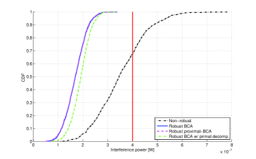
(a) Case (c1)

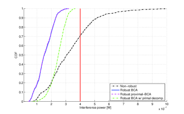
(b) Case (c2)

Figure 2: Interference cumulative distribution function (CDF).

The trajectories provided in Fig. 2 refer to the block coordinate ascent (BCA) algorithm described in Section III; the one with the proximal point-based regularization (proximal-BCA) explained in Section III-C; and the non-robust solver of (P2), where the estimates $\{\hat{\mathbf{G}}_{k}\}$ are used in place of the true channels $\{\mathbf{G}_{k}\}$. Furthermore, the green trajectory corresponds to (P8), where the subgradient projection (54) is implemented at the end of each BCA cycle, which includes $K$ updates of $\mathbf{Q}_{k}$ for $k=1,\ldots,K$. As expected, the proposed robust schemes enforce the interference constraint strictly in both scenarios (c1) and (c2). In fact, the interference never exceeds the tolerable limit shown as the vertical red solid line in Fig. 2. The CDFs corresponding to the proposed BCA and its proximal counterpart nearly coincide. In fact, the two algorithms frequently converge to identical stationary points in this particular simulation setup. Notice that with the primal decomposition approach the beamforming strategy is less conservative. On the contrary, the non-robust approach frequently violates the interference limit (more than $30\%$ of the time). Finally, comparing Fig. 2(a) with Fig. 2(b), one notices that the interference inflicted to the PU under (c1) and the one under (c2) are approximately of the same order. Since in the second case the CR-to-PU distances are smaller, the CR transmitters lower their transmit-powers to protect the PU robustly.

Convergence of the proposed algorithms with given channel realizations and over variable SNRs is illustrated in Fig. 3. It is clearly seen that the total MSEs decrease monotonically across fast-converging iterations, and speed is roughly identical in (c1) and (c2). As expected, the proximal point-based algorithm exhibits a slightly slower convergence rate. Notice also that the primal decomposition method returns improved operational points, especially for medium and low SNR values. Furthermore, the gap between the sum-MSEs obtained with and without the primal decomposition scheme is more evident under (c2). Clearly, the sum-MSEs at convergence in (c2) are higher than the counterparts of (c1). This is because CRs are constrained to use a relatively lower transmit-power in order to enforce the robust interference constraints; this, in turn, leads to higher sum-MSEs and may reduce the quality of the CR-to-CR communications.

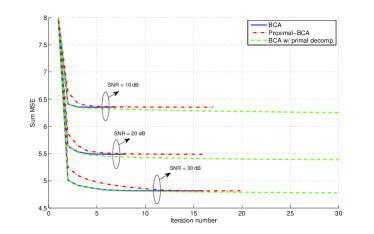
(a) Case (c1)

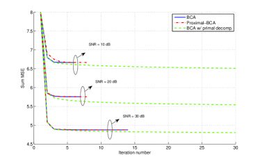
(b) Case (c2)

Figure 3: Convergence of proposed algorithms, for SNR = 10, 20, and 30 dB.

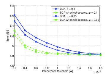
Figure 4: Achieved sum-MSE as a function of $\iota^{\textrm{max}}$, for SNR = 10 dB.

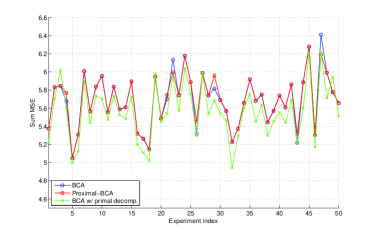
Figure 5: Achieved sum-MSE for SNR = 15 dB.

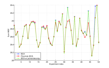
Figure 6: Achieved sum-MSE for SNR = 15 dB.

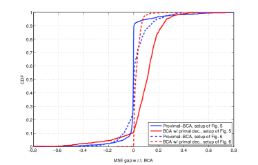
Figure 7: CDF of sum-MSE gaps (relative to the BCA) using proximal-BCA (blue) and primal decomposition (red): $\textrm{MSE}({\textrm{BCA}})-\textrm{MSE}(\textrm{proximal-BCA})$ and $\textrm{MSE}({\textrm{BCA}})-\textrm{MSE}(\textrm{BCA-primal decomp.})$.

In Fig. 4, the achieved sum-MSE at convergence is reported as a function of the total interference threshold. Two sizes of the uncertainty region are considered with $\rho=0.05$ and $\rho=0.1$. Focusing on the first case, it can be seen that the two achieved sum-MSEs first monotonically decrease as the interference threshold increases, and subsequently they remain approximately constant. Specifically, for smaller $\iota^{\textrm{max}}$, the transmit-CRs are confined to relatively low transmit-powers in order to satisfy the interference constraint. On the other hand, for high values of $\iota^{\textrm{max}}$, the interference constraint is no longer a concern, and the attainable sum-MSEs are mainly due to CR self-interference. Notice also that for $\rho=0.1$ the sum-MSEs are clearly higher, although they present a trend similar to the previous case. This is because the uncertainty region in (12c) becomes larger, which results in a higher sum-MSE.

In order to compare performance of the proposed algorithms, the total MSE obtained at convergence is depicted in Fig. 5 for $50$ different experiments. In each experiment, independent channel realizations are generated. The SNR is set to $15$ dB. It is clearly seen that the objectives values of the two proposed methods often coincide. The differences presented in a few experiments are caused by convergence to two different stationary points. In this case, it is certainly convenient to employ the first algorithm, as it ensures faster convergence (see Fig. 3(a)) without appreciable variations in the overall MSE. Notice that a smaller mean-square error can be obtained by resorting to the primal decomposition technique.

In Fig. 6, the simulation setup involves $8$ CR pairs and one PU receiver. The CR transmitters have $4$ antennas, while the receiving CRs and the PU are equipped with $2$ antennas. The distances $d_{k,k}$ are set to $50$ m, while $\{d_{k,j}\}_{k\neq j}$ distances are uniformly distributed in the interval between $30$ and $250$ m. Finally, CR-to-PU distances are uniformly distributed between $100$ and $200$ m. Clearly, matrices $\{\mathbf{H}_{k,k}\}$ here do not have full column rank. It is observed that about $10\%$ of the times the proximal point based algorithm yields smaller values of the sum-MSE than Algorithm 1. This demonstrates that Algorithm 1 may not converge to a stationary point, or, it returns an MSE that is likely to be worse than that of the proximal point-based scheme.

Fig. 7 depicts the CDFs of the difference between the sum-MSE obtained with BCA, along with the ones obtained with proximal-BCA and with the primal decomposition method. The simulation setups of Figs. 5 and 6 are considered. In the first case, it can be seen that for over $80\%$ of the trials the BCA and proximal-BCA methods yield exactly the same solution. Moreover, BCA with primal decomposition performs better than the BCA method about $90\%$ of the time. Specifically, the gain can be up to $0.765$, which corresponds to approximately $14\%$ of the average sum MSE of the BCA. In the second case, the proximal-BCA returns a smaller sum-MSE with higher frequency.

VI Concluding summary

Two beamforming schemes were introduced for underlay MIMO CR systems in the presence of uncertain CR-to-PU propagation channels. Robust interference constraints were derived by employing a norm-bounded channel uncertainty model, which captures errors in the channel estimation phase, or, random fading effects around the deterministic path loss. Accordingly, a robust beamforming design approach was formulated to minimize the total MSE in the information symbol reconstruction, while ensuring protection of the primary system. In order to solve the formulated non-convex optimization problem, a cyclic block coordinate ascent algorithm was developed, and its convergence to a stationary point was established when all CR-to-CR direct channel matrices have full column rank. A second algorithm based on a proximal point regularization technique was also developed. Although slower than the first, the proximal point-based scheme was shown capable of converging to a stationary point even for rank-deficient channel matrices. The two solutions offer complementary strengths as far as convergence rate, computational complexity, and MSE optimality are concerned. They can both afford on-line distributed implementations. Finally, a primal decomposition technique was employed to approximately solve the robust beamforming problem with coupled interference constraints. The developed centralized and distributed algorithms are also suitable for non-CR MIMO ad-hoc networks as well as for conventional downlink or uplink multi-antenna cellular systems.

-A Derivation of the complex gradient matrix (16)

Using that $\frac{\partial\textrm{Tr}\left\{\mathbf{X}^{{\cal H}}\mathbf{A}\right\}}{\partial\mathbf{X}^{*}}=\mathbf{A}$ [39], and letting $[\mathbf{A}]_{mn}$ denote the $(m,n)$-th entry of matrix $\mathbf{A}$, it follows that

$$\frac{\partial[\mathbf{B}_{j}^{{\cal H}}]_{st}}{\partial\mathbf{Q}_{k}^{*}}=\frac{\partial\textrm{Tr}\left\{\mathbf{e}_{s}^{{\cal H}}\mathbf{H}_{j,k}\mathbf{Q}_{k}^{{\cal H}}\mathbf{H}_{j,k}^{{\cal H}}\mathbf{e}_{t}\right\}}{\partial\mathbf{Q}_{k}^{*}}=\mathbf{H}_{j,k}^{{\cal H}}\mathbf{e}_{t}\mathbf{e}_{s}^{{\cal H}}\mathbf{H}_{j,k}$$ (55)

$$\frac{\partial[\mathbf{B}_{j}^{{\cal H}}]_{st}}{\partial[\mathbf{Q}_{k}^{*}]_{mn}}=\mathbf{e}_{m}^{{\cal H}}\mathbf{H}_{j,k}^{{\cal H}}\mathbf{e}_{t}\mathbf{e}_{s}^{{\cal H}}\mathbf{H}_{j,k}\mathbf{e}_{n}=\mathbf{e}_{s}^{{\cal H}}\mathbf{H}_{j,k}\mathbf{e}_{n}\mathbf{e}_{m}^{{\cal H}}\mathbf{H}_{j,k}^{{\cal H}}\mathbf{e}_{t}$$ (56)

which can be written in a compact form as $\frac{\partial\mathbf{B}_{j}^{{\cal H}}}{\partial[\mathbf{Q}_{k}^{*}]_{mn}}=\mathbf{H}_{j,k}\mathbf{e}_{n}\mathbf{e}_{m}^{{\cal H}}\mathbf{H}_{j,k}^{{\cal H}}$. Then, the identity $\frac{\partial f}{\partial\mathbf{X}^{*}}=-\mathbf{X}^{-1}\left(\frac{\partial f}{\partial(\mathbf{X}^{-1})^{*}}\right)\mathbf{X}^{-1}$ [39], which holds for any Hermitian positive definite matrix $\mathbf{X}$, is used to obtain

$$\frac{\partial u_{j}}{\partial\mathbf{B}_{j}^{*}}=-\mathbf{B}_{j}^{-1}\frac{\partial\textrm{Tr}\left\{\mathbf{V}_{j}(\mathbf{B}_{j}^{-1})^{{\cal H}}\right\}}{\partial(\mathbf{B}_{j}^{-1})^{*}}\mathbf{B}_{j}^{-1}=-\mathbf{B}_{j}^{-1}\mathbf{V}_{j}\mathbf{B}_{j}^{-1}.$$ (57)

Using now the chain rule, one arrives at

$$\frac{\partial u_{j}}{\partial[\mathbf{Q}_{k}^{*}]_{mn}} =\textrm{Tr}\left\{\left(\frac{\partial u_{j}}{\partial\mathbf{B}_{j}^{{\cal H}}}\right)^{T}\frac{\partial\mathbf{B}_{j}^{{\cal H}}}{\partial[\mathbf{Q}_{k}^{*}]_{mn}}\right\}$$

$$=\textrm{Tr}\left\{-\mathbf{e}_{m}^{{\cal H}}\mathbf{H}_{j,k}^{{\cal H}}\mathbf{B}_{j}^{-1}\mathbf{V}_{j}\mathbf{B}_{j}^{-1}\mathbf{H}_{j,k}\mathbf{e}_{n}\right\}$$ (58)

which readily leads to the desired result

$$\frac{\partial u_{j}}{\partial\mathbf{Q}_{k}^{*}}=-\mathbf{H}^{{\cal H}}_{j,k}\mathbf{B}_{j}^{-1}\mathbf{V}_{j}\mathbf{B}_{j}^{-1}\mathbf{H}_{j,k}.$$ (59)

-B Proof of Lemma 2

First, convexity of $\mathcal{Q}_{k}$ can be readily proved by the definition of a convex set [18, Ch. 2]. Re-write the function $u_{j}(\mathbf{Q}_{k},\mathbf{Q}_{-k})$ as [cf. (8), (18)]

$$u_{j}(\mathbf{Q}_{k},\mathbf{Q}_{-k})=\textrm{Tr}\left\{\mathbf{V}_{j}^{1/2}\mathbf{P}_{j}^{-1}(\mathbf{Q}_{k})\mathbf{V}_{j}^{1/2}\right\}$$ (60)

where

$$\mathbf{P}_{j}(\mathbf{Q}_{k})=\mathbf{H}_{j,k}\mathbf{Q}_{k}\mathbf{H}_{j,k}^{{\cal H}}+\sum_{i\neq k}\mathbf{H}_{j,i}\mathbf{Q}_{i}\mathbf{H}_{j,i}^{{\cal H}}+\sigma_{j}^{2}\mathbf{I}_{N_{j}}$$

is an affine map with respect to $\mathbf{Q}_{k}$. Since $u_{j}$ is convex in $\mathbf{P}_{j}$ [40, Theorem 2], and convexity is preserved under affine mappings and nonnegative weighted-sums [18, Ch. 3], it follows that $f_{k}(\mathbf{Q}_{k},\mathbf{Q}_{-k})$ is convex in $\mathbf{Q}_{k}$.

-C Proof of Lemma 3

First, notice that the objective function (15a) can be re-written as

$$\widetilde{{\cal U}}_{k}(\mathbf{Q}_{k})= N_{k}+\textrm{Tr}\left\{\mathbf{D}_{k}^{{\cal H}}\mathbf{Q}_{k}\right\}$$

$$-\textrm{Tr}\left\{\mathbf{R}_{k,k}\left(\mathbf{H}_{k,k}\mathbf{Q}_{k}\mathbf{H}^{{\cal H}}_{k,k}+\mathbf{R}_{k,k}\right)^{-1}\right\}.$$ (61)

Then, it suffices to prove strict convexity in $\mathbf{Q}_{k}$ of the third term on the right hand side of (61). This is equivalent to showing that (subscripts are dropped for brevity)

$$J(t):=\textrm{Tr}\left\{\mathbf{R}\left(\mathbf{H}\mathbf{Q}\mathbf{H}^{{\cal H}}+\mathbf{R}\right)^{-1}\right\}$$ (62)

is strictly convex in $t\in\{t|\mathbf{Q}:=\mathbf{X}+t\mathbf{Y}\in{\cal Q}\}$ for any given $\mathbf{X}\in\mathbb{H}^{n\times n}_{+}$ and nonzero $\mathbf{Y}\in\mathbb{H}^{n\times n}$.

To this end, consider the second-order derivative of ${J}(t)$, which is given by

$$\ddot{J}(t)=2\textrm{Tr}\{\mathbf{C}\mathbf{R}\mathbf{C}\mathbf{L}\mathbf{C}\mathbf{L}\}$$ (63)

where $\mathbf{C}:=\left(\mathbf{R}+\mathbf{H}(\mathbf{X}+t\mathbf{Y})\mathbf{H}^{{\cal H}}\right)^{-1}$ and $\mathbf{L}:=\mathbf{H}\mathbf{Y}\mathbf{H}^{{\cal H}}$. Note that matrix $\mathbf{C}\mathbf{R}\mathbf{C}$ is Hermitian positive definite, since $\mathbf{C}$ and $\mathbf{R}$ are Hermitian positive definite too. With $\mathbf{H}$ full column rank, it readily follows that $\mathbf{L}\neq\mathbf{0}$ for any $\mathbf{Y}\neq\mathbf{0}$. This ensures that the Hermitian positive semi-definite matrix $\mathbf{L}\mathbf{C}\mathbf{L}$ is not an all-zero matrix, i.e., $\mathbf{L}\mathbf{C}\mathbf{L}\neq\mathbf{0}$.

Let $\nu_{1}\geq\nu_{2}\geq\cdots\geq\nu_{N}>0$ and $\mu_{1}\geq\mu_{2}\geq\cdots\geq\mu_{N}\geq 0$ denote the eigenvalues of matrices $\mathbf{C}\mathbf{R}\mathbf{C}$ and $\mathbf{L}\mathbf{C}\mathbf{L}$, respectively. Since matrix $\mathbf{L}\mathbf{C}\mathbf{L}\neq\mathbf{0}$, $\mu_{1}$ is strictly positive, and thus

$$\ddot{J}(t) \geq 2\sum_{i=1}^{N}\nu_{i}\mu_{N-i+1}$$ (64a)

$$\geq 2\nu_{N}\mu_{1}>0$$ (64b)

where (64a) follows from von Neumann’s trace inequality [41]. Finally,  (64b) shows the strong convexity (and hence strict convexity) of $J(t)$.

For completeness, we provide an alternative proof of the lemma. With some manipulations, function $h(\mathbf{Q}):=\textrm{Tr}\left\{\mathbf{R}\left(\mathbf{H}\mathbf{Q}\mathbf{H}^{{\cal H}}+\mathbf{R}\right)^{-1}\right\}$ can be re-expressed as

$$h(\mathbf{Q}) =g(\mathbf{R}^{-1/2}\mathbf{H}\mathbf{Q}\mathbf{H}^{{\cal H}}\mathbf{R}^{-1/2})$$

$$=\textrm{Tr}\left\{\left(\mathbf{I}+\mathbf{R}^{-1/2}\mathbf{H}\mathbf{Q}\mathbf{H}^{{\cal H}}\mathbf{R}^{-1/2}\right)^{-1}\right\}$$ (65)

where $g(\mathbf{X}):=\textrm{Tr}\left\{\left(\mathbf{I}+\mathbf{X}\right)^{-1}\right\}$. Let $\lambda_{1}(\mathbf{X}),\ldots,\lambda_{n}(\mathbf{X})$ denote again the eigenvalues of a matrix $\mathbf{X}$. Note that the spectral function $g(\mathbf{X})=s(\lambda(\mathbf{X})):=\sum_{i}\left(\frac{1}{1+\lambda_{i}(\mathbf{X})}\right)$ is strictly convex if and only if the corresponding symmetric function $s(\cdot)$ is strictly convex [42]. To this end, the strict convexity of $\frac{1}{1+x}$ for $x\geq 0$ implies the strict convexity of $s(\cdot)$, and thus of $g(\mathbf{X})$. Under the condition of full column rank of $\mathbf{H}$, we will show that strict convexity is preserved under the linear mapping in (65). Specifically, define

$$\check{\mathbf{Q}}_{i}:=\mathbf{R}^{-1/2}\mathbf{H}\mathbf{Q}_{i}\mathbf{H}^{{\cal H}}\mathbf{R}^{-1/2},\,i=1,2.$$

Then, for any $\mathbf{Q}_{1}\neq\mathbf{Q}_{2}\in{\cal Q}$ and $0<\lambda<1$, we have that

$$h(\lambda\mathbf{Q}_{1}+(1-\lambda)\mathbf{Q}_{2}) =g(\lambda\check{\mathbf{Q}}_{1}+(1-\lambda)\check{\mathbf{Q}}_{2})$$ (66a)

$$<\lambda g(\check{\mathbf{Q}}_{1})+(1-\lambda)g(\check{\mathbf{Q}}_{2})$$ (66b)

$$=\lambda h(\mathbf{Q}_{1})+(1-\lambda)h(\mathbf{Q}_{2})$$ (66c)

where (66b) follows from the strict convexity of $g(\cdot)$, and the fact that $\check{\mathbf{Q}}_{1}\neq\check{\mathbf{Q}}_{2}$ holds for any $\mathbf{Q}_{1}\neq\mathbf{Q}_{2}$, since $\mathbf{H}$ is full column rank.

References

• [1] Q. Zhao and B. M. Sadler, “A survey of dynamic spectrum access,” IEEE Sig. Proc. Mag., vol. 24, no. 3, pp. 79–89, May 2007.
• [2] S.-J. Kim, E. Dall’Anese, and G. B. Giannakis, “Cooperative spectrum sensing for cognitive radios using kriged Kalman filtering,” IEEE J. Sel. Topics Sig. Proc., vol. 5, no. 1, pp. 24–36, Feb. 2011.
• [3] J. Font-Segura and X. Wang, “GLRT-based spectrum sensing for cognitive radio with prior information,” IEEE Trans. Commun., vol. 58, no. 7, pp. 2137–2146, July 2010.
• [4] S. S. Christensen, R. Agarwal, E. de Carvalho, and J. M. Cioffi, “Weighted sum-rate maximization using weighted MMSE for MIMO-BC beamforming design,” IEEE Trans. Wireless Commun., vol. 7, no. 12, pp. 4792–4799, Dec. 2008.
• [5] M. Razaviyayn, M. Sanjabi, and Z.-Q. Luo, “Linear transceiver design for interference alignment: Complexity and computation,” IEEE Trans. Info. Theory, vol. 58, no. 5, pp. 2896–2910, May 2012.
• [6] M. Ding and S. D. Blostein, “MIMO minimum total MSE transceiver design with imperfect CSI at both ends,” IEEE Trans. Sig. Proc., vol. 57, no. 3, pp. 1141–1150, Mar. 2009.
• [7] N. Vucic, H. Boche, and S. Shi, “Robust transceiver optimization in downlink multiuser MIMO systems,” IEEE Trans. Sig. Proc., vol. 57, no. 9, pp. 3576–3587, Sept. 2009.
• [8] R. Zhang and Y.-C. Liang, “Exploiting multi-antennas for opportunistic spectrum sharing in cognitive radio networks,” IEEE J. Sel. Topics Sig. Proc., vol. 2, no. 1, pp. 88–102, Feb. 2008.
• [9] L. Zhang, Y.-C. Liang, and Y. Xin, “Joint beamforming and power allocation for multiple access channels in cognitive radio networks,” IEEE J. Sel. Areas Commun., vol. 26, no. 1, pp. 38–51, Jan. 2008.
• [10] S.-J. Kim and G. B. Giannakis, “Optimal resource allocation for MIMO ad hoc cognitive radio networks,” IEEE Trans. Info. Theory, vol. 57, no. 5, pp. 3117–3131, May 2011.
• [11] G. Scutari and D. P. Palomar, “MIMO cognitive radio: A game-theoretical approach,” IEEE Trans. Sig. Proc., vol. 58, no. 2, pp. 761–780, Feb. 2010.
• [12] E. Dall’Anese, S.-J. Kim, G. B. Giannakis, and S. Pupolin, “Power control for cognitive radio networks under channel uncertainty,” IEEE Trans. Wireless Commun., vol. 10, no. 10, pp. 3541–3551, Oct. 2011.
• [13] E. A. Gharavol, Y.-C. Liang, and K. Mouthaan, “Robust downlink beamforming in multiuser MISO cognitive radio networks with imperfect channel-state information,” IEEE Trans. Veh. Technol., vol. 59, no. 6, pp. 2852–2860, July 2010.
• [14] G. Zheng, K.-K. Wong, and B. Ottersten, “Robust cognitive beamforming with bounded channel uncertainties,” IEEE Trans. Sig. Proc., vol. 57, no. 12, pp. 4871–4881, Dec. 2009.
• [15] E. A. Gharavol, Y.-C. Liang, and K. Mouthaan, “Robust linear transceiver design in MIMO ad hoc cognitive radio networks with imperfect channel state information,” IEEE Trans. Wireless Commun., vol. 10, no. 5, pp. 1448–1457, May 2011.
• [16] T. Al-Khasib, M. Shenouda, and L. Lampee, “Dynamic spectrum management for multiple-antenna cognitive radio systems: Designs with imperfect CSI,” IEEE Trans. Wireless Commun., vol. 10, no. 9, pp. 2850–2859, Sept. 2011.
• [17] J. Wang, G. Scutari, and D. P. Palomar, “Robust MIMO cognitive radio via game theory,” IEEE Trans. Sig. Proc., vol. 59, no. 3, pp. 1183–1201, Mar. 2011.
• [18] S. Boyd and L. Vandenberghe, Convex Optimization.   Cambridge University Press, 2004.
• [19] D. P. Bertsekas and J. N. Tsitsiklis, Parallel and Distributed Computation: Numerical Methods.   Belmont, MA: Athena Scientific, 1997.
• [20] J. P. Kermoal, L. Schumacher, K. I. Pedersen, P. E. Mogensen, and F. Frederiksen, “A stochastic MIMO radio channel model with experimental validation,” IEEE J. Sel. Areas Commun., vol. 20, no. 6, pp. 1211–1226, Aug. 2002.
• [21] R. T. Rockafellar, “Augmented Lagrangians and applications of the proximal point algorithms in convex programming,” Math. Oper. Res., vol. 1, pp. 97 –116, 1976.
• [22] D. P. Palomar, J. M. Cioffi, and M. A. Lagunas, “Joint Tx-Rx beamforming design for multicarrier MIMO channels: A unified framework for convex optimization,” IEEE Trans. Sig. Proc., vol. 51, no. 9, pp. 2381–2401, Sept. 2003.
• [23] C. W. Tan, M. Chiang, and R. Srikant, “Maximizing sum rate and minimizing MSE on multiuser downlink: Optimality, fast algorithms and equivalence via max-min SINR,” IEEE Trans. Sig. Proc., vol. 59, no. 12, pp. 6127–6143, Dec. 2011.
• [24] L. Zhang, Y.-C. Liang, Y. Xin, and H. V. Poor, “Robust cognitive beamforming with partial channel state information,” IEEE Trans. Wireless Commun., vol. 8, no. 8, pp. 4143–4153, Aug. 2009.
• [25] M. Biguesh and A. B. Gershman, “Training-based MIMO channel estimation: A study of estimator tradeoffs and optimal training signals,” IEEE Trans. Sig. Proc., vol. 54, no. 3, pp. 884–893, Mar. 2006.
• [26] M. Shenouda and T. N. Davidson, “On the design of linear transceivers for multiuser systems with channel uncertainty,” IEEE J. Sel. Areas Commun., vol. 26, no. 6, pp. 1015–1024, Aug. 2008.
• [27] A. L. Yuille and A. Rangarajan, “The concave-convex procedure,” Neural Computation, vol. 15, no. 4, pp. 915–936, Apr. 2003.
• [28] D. R. Hunter and K. Lange, “A tutorial on MM algorithms,” The American Statistician, vol. 58, no. 1, pp. 30–37, Feb. 2004.
• [29] D. P. Bertsekas, Nonlinear Programming, 2nd ed.   Belmont, MA: Athena Scientific, 1999.
• [30] E. Dall’Anese, S.-J. Kim, and G. B. Giannakis, “Channel gain map tracking via distributed kriging,” IEEE Trans. Veh. Technol., vol. 60, no. 3, pp. 1205–1211, Mar. 2011.
• [31] Kyoung-Lae Noh, E. Serpedin, and K. Qaraqe, “A new approach for time synchronization in wireless sensor networks: Pairwise broadcast synchronization,” IEEE Trans. Wireless Commun., vol. 7, no. 9, pp. 3318–3322, Sept. 2008.
• [32] D. Zennaro, E. Dall’Anese, T. Erseghe, and L. Vangelista, “Fast clock synchronization in wireless sensor networks via ADMM-based consensus,” in Proc. of Intl. Sym. on Mod. and Opt. in Mobile, Ad Hoc and Wireless Net., Princeton, NJ, United States, May 2011, pp. 148–153.
• [33] C. H. Rentel and T. Kunz, “A mutual network synchronization method for wireless ad hoc and sensor networks,” IEEE Trans. Mobile Comput., vol. 7, no. 5, pp. 633–646, 2008.
• [34] D. P. Bertsekas, Convex optimization theory.   Belmont, MA: Athena Scientific, 2009.
• [35] L. Grippo and M. Sciandrone, “On the convergence of the block nonlinear Gauss–Seidel method under convex constraints,” Operations Research Letters, vol. 26, no. 3, pp. 127–136, Apr. 2000.
• [36] D. P. Palomar, “Convex primal decomposition for multicarrier linear MIMO transceivers,” IEEE Trans. Sig. Proc., vol. 53, no. 12, pp. 4661–4674, Dec. 2005.
• [37] M. Grant and S. Boyd, “CVX: Matlab software for disciplined convex programming, version 1.21,” http://cvxr.com/cvx/, Apr. 2011.
• [38] J. F. Sturm, “Using SeDuMi 1.02, a MATLAB toolbox for optimization over symmetric cones,” Optim. Meth. Softw., vol. 11 -12, pp. 625 –653, Aug. 1999.
• [39] J. R. Magnus and H. Neudecker, Matrix Differential Calculus with Applications in Statistics and Economics, 2nd ed.   New York: Wiley, 1999.
• [40] E. H. Lieb, “Convex trace functions and the Wigner-Yanase-Dyson conjecture,” Advances in Math., vol. 11, no. 3, pp. 267–288, Dec. 1973.
• [41] L. Mirsky, “On the trace of matrix products,” Mathematische Nachrichten, vol. 20, no. 3–6, pp. 171–174, 1959.
• [42] C. Davis, “All convex invariant functions of Hermitian matrices,” Arch. Math., vol. 8, no. 4, pp. 276 –278, Feb. 1957.