Measurement of the CMB Polarization at 95 GHz from QUIET

Abstract

Despite the great success of precision cosmology, cosmologists cannot fully explain the initial conditions of the Universe. Inflation, an exponential expansion in the first $\approx 10^{-36}$ s, is a promising potential explanation. A generic prediction of inflation is odd-parity (B-mode) polarization in the cosmic microwave background (CMB). The Q/U Imaging ExperimenT (QUIET) aimed to limit or detect this polarization.

We built a coherent pseudo-correlation microwave polarimeter. An array of mass-produced “modules” populated the focal plane of a 1.4-m telescope. Each module had a sensitivity to polarization of 756 $\mu$K$\sqrt{\textrm{s}}$ with a bandwidth of $10.7\pm 1.1$ GHz centered at $94.5\pm 0.8$ GHz; the combined sensitivity was $87\pm 7\,\mu$K$\sqrt{\textrm{s}}$. We incorporated “deck” rotation, an absorbing ground screen, a new time-stream “double-demodulation” technique, and optimized optics into the design to reduce instrumental polarization. We observed with this instrument at the Atacama Plateau in Chile between August 2009 and December 2010. We collected 5336.9 hours of CMB observation and 1090 hours of astronomical calibration.

This thesis describes the analysis and results of these data. We characterized the instrument using the astronomical calibration data as well as purpose-built artificial sources. We developed noise modeling, filtering, and data selection following a blind-analysis strategy. Central to this strategy was a suite of 32 null tests, each motivated by a possible instrumental problem or systematic effect. We also evaluated the systematic errors in the blind stage of the analysis before the result was known. We then calculated the CMB power spectra using a pseudo-$C_{\ell}$ cross-correlation technique that suppressed contamination and made the result insensitive to noise bias. We measured the first three peaks of the E-mode spectrum at high significance and limited B-mode polarization ($r=1.48^{+1.06}_{-0.92}$ at 68% confidence and $r<3.3$ at 95% confidence). Systematic errors were well below ($r<0.01$) our B-mode polarization limit. This systematic-error reduction was a strong demonstration of technology for application in more sensitive, next-generation CMB experiments.

to Mr. Wallin, who never doubted

and

to Bruce, who made it possible

Here friend, have this!
Okay, thanks.

Team Potato

I could never have written this thesis without the support of many people. Here I thank as many as memory will permit.

First thanks go to my adviser Bruce Winstein, who was also the PI of QUIET. Without him I never would have gotten involved in CMB physics. Bruce taught me how to be a really careful scientist. He was also incredibly generous with his time and resourceful at getting me whatever I needed to get that science done. My greatest regret is that he never got to see this work finished.

My adviser Stephan Meyer stepped in at a time when we were all reeling from Bruce’s death. Steve helped me understand all the things I thought I understood—but didn’t. Steve was also really good at keeping me focused on the next steps at every stage in this process.

Akito Kusaka took on responsibility beyond what is normally expected of a post-doc. He kindly pointed out mistakes in every memo I sent him. Any ones remaining here are my own.

My thesis committee, Paolo Privitera, Michael Turner, and David Biron, provided many insightful comments and suggestions. This thesis is much better as a result.

Thanks to the rest of the Chicago QUIET group, Colin Bischoff, Alison Brizius, Yuji Chinone, Dan Kapner, and Osamu Tajima, for keeping things fun. My Fermilab colleagues, Hogan Nguyen and Donna Kubik, kept up the enthusiasm when the Chicago team was burnt out.

Thanks to the Q-band deployment team for putting up with me even when I was too low on oxygen to make any sense. Special thanks to the engineers and technician who maintained and operated the telescope, José Cortés, Cristobal Jara, Freddy Muñoz, and Carlos Verdugo. Without them, we never would have gotten past the first mount stall. Thanks also to the other Atacama experiments, especially APEX, ACT, and ALMA, for supporting our operations in divers ways.

Thanks to everyone else in the QUIET Collaboration for numerous comments, discussions, and a whole lot of science.

My office mates, Cora Dvorkin, Sam Leitner, Denis Erkal, and Yin Li, provided job-seeking support, laughs, and daily encouragement.

Thanks to my classmates and friends in Chicago, who were uniformly, point-wise, and L2 supportive. Thanks to my Tpot friends, whose support was neither closed nor bounded.

My family thought I was doing something worthwhile, even when they didn’t understand it.

Some work was performed on the Joint Fermilab-KICP Supercomputing Cluster, supported by grants from Fermilab, the Kavli Institute for Cosmological Physics, and the University of Chicago. Some work was performed on the Central Computing System, owned and operated by the Computing Research Center at KEK. This research used resources of the National Energy Research Scientific Computing Center, which is supported by the Office of Science of the U.S. Department of Energy under Contract No. DE-AC02-05CH11231. Some of the results in this paper have been derived using the HEALPix (gorski_healpix) package.

Last and least, I thank the mount, which lasted much longer than anyone thought it would.

Chapter 1 Introduction

In the beginning the Universe was created. This has made a lot of people very angry and been widely regarded as a bad move.

Douglas Adams

Q/U Imaging ExperimenT (QUIET) measured the cosmic microwave background (CMB) polarization with the goal of constraining a signal from inflation. The standard model of cosmology begins with inflation, an accelerated expansion of the Universe in the first $\approx 10^{-36}$ s that sets its initial conditions. Inflation generated a stochastic background of gravitational waves. These gravitational waves created a small polarization anisotropy in the CMB, the radiation released when the early Universe became un-ionized. We measured the CMB polarization and isolated the signal potentially bearing evidence of inflation. This thesis describes the QUIET instrument, observations, data analysis, and results including a limit ($r<3.3$) on the inflation signal.

1.1 Inflationary Cosmology

Inflation provides the initial conditions for the standard model of cosmology ($\Lambda$CDM, see e.g. ryden). In the standard model, the Universe is assumed to be homogeneous and isotropic on large scales ($\gtrsim 100$ Mpc). In General Relativity, these conditions require a metric of the form

$$ds^{2}=-c^{2}dt^{2}+a(t)^{2}\left(dx^{2}+dy^{2}+dz^{2}\right).$$ (1.1)

This form is only valid for a nearly flat Universe, one of the assumptions of the standard model. The Universe expanded from a hot, dense initial state; thus $a(t)$ increases with time. In addition to the background metric, the standard model specifies the energy content and how it behaves. The evolution is governed by

$$\left(\frac{1}{a}\frac{da}{dt}\right)^{2} = \frac{8\pi G}{3c^{2}}\rho$$ (1.2)

$$\frac{1}{a}\frac{d^{2}a}{dt^{2}} = -\frac{4\pi G}{3c^{2}}(\rho+3p),$$ (1.3)

where $\rho$ is the energy density and $p$ is the pressure.

Inflation was originally proposed by guth_inflation to explain puzzling observations (see also §1.2): the Universe is homogeneous even across regions that were causally disconnected. The Universe is (almost) flat, but a nearly flat Universe is an unstable solution. Guth’s final motivation was the absence of magnetic monopoles, which are generally expected in grand unified theories. The generation of initial density perturbations is an additional motivation for an inflationary origin.

Although there are many models for the details of inflation, a simple, single-field, slow-roll model demonstrates the general features important for this thesis. Suppose there is a scalar field $\phi$ with mass $m$ and potential

$$V(\phi)=m^{2}\phi^{2}/2.$$ (1.4)

The corresponding equations of motion are

$$\ddot{\phi}+3H\dot{\phi}=-m^{2}\phi$$ (1.5)

and

$$H^{2}+\frac{k}{a^{2}}=\left(\dot{\phi}^{2}+m^{2}\phi^{2}\right)/6,$$ (1.6)

where $k$ is $-1$, 0, or 1 for an open, flat, or closed Universe, respectively. An overdot denotes a derivative with respect to time coordinate $t$, and $H\equiv\dot{a}/a$. If the initial value of $\phi$ is $\gg 1$ then the evolution is in the “slow-roll” regime with

$$\ddot{\phi}\ll 3H\dot{\phi},$$ (1.7)

$$H^{2}\gg k/a^{2},$$ (1.8)

and

$$\dot{\phi}^{2}\ll m^{2}\phi^{2}.$$ (1.9)

Eq. 1.8 implies that spatial curvature becomes negligible. In this regime the equations of motion simplify to

$$H=m\phi/\sqrt{6}$$ (1.10)

and

$$\dot{\phi}=-m\sqrt{2/3}.$$ (1.11)

In the slow-roll regime, the change of $\phi$ is negligible so

$$a(t)=e^{Ht}=e^{m\phi t/\sqrt{6}}.$$ (1.12)

This exponential expansion continues until $\phi\approx 1$. If the initial scale factor and field values are $a_{0}$ and $\phi_{0}$, respectively, then the total expansion caused by inflation is

$$a/a_{0}=e^{\phi_{0}^{2}/4}.$$ (1.13)

This model can explain the “puzzling observations” above. For realistic $m\approx 10^{-6}$, $a/a_{0}\approx 10^{10^{10}}$. This expansion occurred in $\approx 10^{-36}$ s. Under a “worst case” assumption that the Universe before inflation had radius of curvature approximately the Planck length ($10^{-33}$ cm), after inflation it would grow to $\approx 10^{10^{10}}$ cm. This is much larger than the present observable Universe, $10^{28}$ cm. Thus all observations cosmologists have made correspond to a small patch that was a tiny fraction of the total volume of the initial Universe and easily causally connected. The initial curvature is now unobservable because the present radius of curvature is much larger than any scale we can observe. For similar reasons, the expansion erases any evidence of initial inhomogeneity and so reduces the density of monopoles that it is unlikely to find one in our Hubble volume. At the end of inflation, $\phi$ decays into other elementary particles which interact and eventually reach thermal equilibrium.

Due to quantum fluctuations there were perturbations in the scalar field

$$\delta\phi\approx\frac{H}{2\pi}.$$ (1.14)

Differences in the value of $\phi$ caused inflation to end slightly earlier or later than the average value. The change in the time of the end of inflation is

$$\delta t=\delta\phi/\dot{\phi}\approx\frac{H}{2\pi\dot{\phi}}.$$ (1.15)

From Eq. 1.2,

$$\rho\propto H^{2}.$$ (1.16)

After the end of inflation, the Universe was radiation-dominated so

$$H\propto t^{-1}.$$ (1.17)

Combining Eqs. 1.14–1.17,

$$\delta H/H\approx\delta t/t\approx\delta\rho/\rho\approx\frac{H^{2}}{2\pi\dot{\phi}}.$$ (1.18)

The perturbation amplitude for a given wavelength depends on the fluctuations occurring when that wavelength was comparable to the horizon size. Since $\frac{H^{2}}{2\pi\dot{\phi}}$ changed slowly during the slow-roll regime, the spectrum of initial perturbations was nearly scale-invariant. Thus the combination of inflation and quantum fluctuations naturally produced the small anisotropy we observe today.

In addition to the density perturbations, inflation will in general create tensor perturbations (gravitational waves). I adopted the convention (wmap7_cosmology)

$$\Delta^{2}_{R}(k) \equiv \frac{k^{3}<|R_{k}|^{2}>}{2\pi^{2}}=\Delta^{2}_{R}(k_{0})\left(k/k_{0}\right)^{n_{s}-1}$$ (1.19)

$$\Delta_{h}^{2}(k) \equiv \frac{4k^{3}<|h_{k}|^{2}>}{2\pi^{2}}=\Delta_{h}^{2}(k_{0})\left(k/k_{0}\right)^{n_{t}}$$ (1.20)

for nearly scale-invariant spectra, where $R_{k}$ is a perturbation of the scalar curvature with comoving wavenumber $k$, $k_{0}$ is a pivot scale, $n_{s}$ is the scalar spectral index, $h_{k}$ is a tensor perturbation, and $n_{t}$ is the tensor spectral index.

There is no observational evidence for tensor perturbations; however, many inflationary models predict them. The tensor-to-scalar ratio

$$r\equiv\frac{\Delta^{2}_{h}(k_{0})}{\Delta^{2}_{R}(k_{0})}$$ (1.21)

is a figure of merit for comparing tensor-perturbation searches and comparing experimental results to different inflationary models. In the slow-roll regime,

$$r=16\epsilon\equiv 8\left(\frac{1}{V}\frac{dV}{d\phi}\right)^{2}.$$ (1.22)

In the $V=m^{2}\phi^{2}/2$ model, $r=32/\phi^{2}$. Using Eq. 1.13, $r=8/N$, where $N$ is the number of e-folds of inflation for scales corresponding to the size of the observable Universe. For typical $N\approx 60$, $r\approx 0.13$. Regardless of the model, detection of non-zero $r$ would be new, strong evidence for inflation. Moreover, a measurement of $r$ would give information about the energy scale of inflation (Liddle19931; baumann_cmbpol)

$$V^{1/4}=1.06\times 10^{16}\textrm{~{}GeV~{}}(r/0.01)^{1/4}.$$ (1.23)

The best existing limit is $r<0.2$ (wmap7_cosmology). For reasons that will be explained below (§1.2.2), only $r\gtrsim 0.001$ is detectable in CMB polarization. Therefore, a measurement of $r$ would indicate that inflation occurred at an energy comparable to the grand unification scale of particle physics. Although models with arbitrarily small $r$ exist, current evidence and naturalness considerations suggest $r\geq 0.01$ (Boyle06). Thus we, along with many other cosmologists, are interested in detecting tensor perturbations from inflation and measuring $r$ from CMB observations.

1.2 The Cosmic Microwave Background

The CMB is relic radiation from when the Universe was younger and hotter. The CMB was created when the formation of Hydrogen made the Universe transparent to photons. By observing this radiation, cosmologists learn about the conditions of the early Universe. The small anisotropy in the radiation intensity has constrained cosmological models. The CMB polarization is the current frontier for probes of inflation because it has the smallest contaminating signals.

The CMB was formed at redshift $z\approx 1100$ when the temperature became low enough (3000 K) for the ionization fraction to decrease rapidly. Once the Universe was un-ionized, the photon mean free path became much greater than the Hubble volume. Most CMB photons last scattered at the time of recombination. Thus the measured properties of the CMB directly correspond to early Universe physics. The CMB has a blackbody spectrum (fixsen_firas) with temperature $T_{\textrm{cmb}}=2.72548\pm 0.00057$ K (Fixsen_cmb_09). Spatially, the CMB is nearly uniform with $\Delta T/T\approx 10^{-5}$ (smoot_dmr). These small anisotropies are the result of the initial perturbations from inflation modulated by plasma physics at recombination (Hu:2001bc; scott_review).

1.2.1   CMB Measurements and Their Implications

CMB measurements, particularly of the temperature anisotropy, are one of the observational foundations of the standard cosmological model. The basic result of a temperature anisotropy experiment is a map of the CMB temperature $T(\theta,\phi)$. To extract the cosmologically relevant information, cosmologists typically decompose the map in spherical harmonics

$$\sum_{\ell,m}a_{\ell m}Y_{\ell m}(\theta,\phi)=T(\theta,\phi).$$ (1.24)

If the fluctuations are Gaussian and isotropic then all cosmological information is contained in the power spectrum

$$C_{\ell}\equiv~{}<|a_{\ell m}^{2}|>.$$ (1.25)

At low $\ell$ ($\lesssim 100$) the Sachs–Wolfe effect (sachs_wolfe) dominates, and $C_{\ell}\ell(\ell+1)$ is nearly constant. At $\ell\gtrsim 100$, the oscillations of the photon–baryon fluid create acoustic peaks. At $\ell\gtrsim 1000$, the non-zero width of the last-scattering surface damps the anisotropies.

Cosmologists can only observe a single realization of the sky. At each $\ell$ there are only $2\ell+1$ modes. Thus any measurement of the ensemble average $C_{\ell}$ has an irreducible sample variance $\frac{2}{2\ell+1}C_{\ell}^{2}$. Moreover, practical experiments only cover a fraction of the sky, $f_{\textrm{sky}}<1$. Limited sky fraction reduces the effective number of modes measured so the sample variance increases to $\frac{1}{f_{\textrm{sky}}}\frac{2}{2\ell+1}C_{\ell}^{2}$ (scott94). Sample variance fundamentally limits the cosmological information that can be extracted from the CMB.

Existing CMB observations (quad_2009; bicep_2009; wmap7_spectra; Reichardt:2011yv; Keisler:2011aw; Dunkley:2010ge) combined with other observations (especially, galaxy clusters, weak gravitational lensing, supernova luminosity distances, and baryon acoustic oscillations (BAO). See e.g. wmap7_cosmology for combined analyses) have shown that

1. The Universe is nearly flat. wmap7_cosmology measured the curvature fraction $-0.0133<\Omega_{k}<0.0084$.

2. The initial perturbations were Gaussian and adiabatic (within measurement uncertainty).

3. The spectral index $n_{s}$ is almost, but not exactly 1.

4. The initial perturbations at a given wavelength were in phase (Dodelson:2003ip).

5. The Universe became un-ionized at $z\approx 1100$ and reionized at $z\approx 10$.

6. The current energy of the Universe is in dark energy ($72.8^{+1.5}_{-1.6}$%) and dark matter ($22.7\pm 1.4$%).

7. Structure formed from small initial perturbations which grew because of gravitational collapse.

These observations form the basis for the standard model of cosmology. Particularly, inflation predicts 1–4. To provide even more compelling evidence, we searched for the signal inflation generates in the CMB polarization.

1.2.2   CMB Polarization Measurements

The CMB is partially polarized (hu_white_review; Hu:2001bc). During decoupling, the quadrupole anisotropy in the local temperature led to a net linear polarization of the scattered radiation (Figure 1.1). In Thomson scattering, incoming radiation polarized parallel to the outgoing direction does not contribute to scattering. If the incoming radiation were isotropic, there would be no net polarization. Because the incoming radiation had a quadrupole anisotropy, the intensity was different in the two outgoing polarization states.

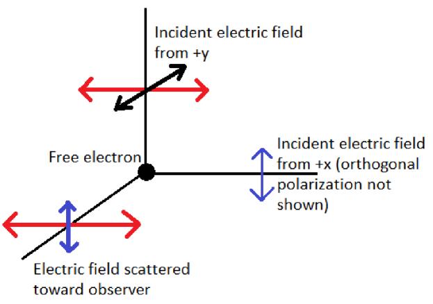
Figure 1.1: Quadrupole temperature anisotropies at decoupling created linear polarization in the CMB. Because electromagnetic waves are transverse, only one polarization state from the $y$ direction can scatter toward us ($z$ direction). Therefore if there was a difference in the electric field amplitudes in the $x$ and $y$ directions (equivalent to a radiation temperature difference), the scattered radiation will be polarized even though the incident radiation was not.

The Stokes parameters

$$I = LL^{*}+RR^{*}$$ (1.26)

$$Q = 2\Re[L^{*}R]$$ (1.27)

$$U = -2\Im[L^{*}R]$$ (1.28)

$$V = LL^{*}-RR^{*}$$ (1.29)

quantify the polarization properties of an electric field with components $E_{x}$ and $E_{y}$. For later convenience I have introduced circular polarization components

$$L=\frac{E_{x}+iE_{y}}{\sqrt{2}}$$ (1.30)

and

$$R=\frac{E_{x}-iE_{y}}{\sqrt{2}};$$ (1.31)

although the net circular polarization ($V$) is negligible for the CMB in theory (cooray_circular_polarization). The Stokes parameters depend on the choice of coordinates. If the coordinate system is rotated by an angle $\psi$ so that $x\rightarrow x^{\prime}$ and $y\rightarrow y^{\prime}$,

$$Q^{\prime} = Q\cos{2\psi}+U\sin{2\psi}$$ (1.32)

$$U^{\prime} = -Q\sin{2\psi}+U\cos{2\psi}.$$ (1.33)

The quantity

$$(Q\pm iU)^{\prime}=e^{\mp 2i\psi}(Q\pm iU)$$ (1.34)

has spin $\pm 2$, and I decomposed it into

$$Q\pm iU=\sum_{\ell,m}a^{\pm}_{\ell m}Y^{\pm}_{\ell m}$$ (1.35)

with spin-2 spherical harmonics $Y^{\pm}$. (The superscripts in $a^{\pm}$ are part of the names of the expansion coefficients, not exponents.) The linear combinations

$$a^{E}_{\ell m} = -\frac{a^{+}_{\ell m}+a^{-}_{\ell m}}{2}$$ (1.36)

$$a^{B}_{\ell m} = i\frac{a^{+}_{\ell m}-a^{-}_{\ell m}}{2}$$ (1.37)

have definite parity: $a^{E}$ (E mode) has even parity and $a^{B}$ (B mode) has odd parity. The corresponding power spectra are

$$C^{EE}_{\ell} = ~{}<a^{E*}_{\ell m}a^{E}_{\ell m}>$$ (1.38)

$$C^{BB}_{\ell} = ~{}<a^{B*}_{\ell m}a^{B}_{\ell m}>$$ (1.39)

$$C^{EB}_{\ell} = ~{}<a^{E*}_{\ell m}a^{B}_{\ell m}>.$$ (1.40)

Since E and B modes have different parity, $C^{EB}_{\ell}=0$ unless there is parity violation. For the same reason, primordial scalar perturbations do not produce B modes. However, tensor perturbations produce both E and B modes. Since $r$ is small, scalar perturbations gave the dominant contribution to $C^{EE}_{\ell}$. Therefore $C^{BB}_{\ell}$ is the most promising for a search for inflationary tensor perturbations.

Many experiments have measured non-zero $C^{EE}_{\ell}$ (dasi_first_detection; cbi_2005; capmap_season3; quad_2009; bicep_2009; quiet_qband_result), and the results agreed with the standard cosmological model. No experiment has detected B modes. The best upper limit on inflationary B modes is $r<0.72$ (bicep_2009). Our main science goal in QUIET was to improve this limit. Astrophysical foregrounds make it extremely difficult to detect $r\lesssim 0.001$ (cmbpol_foreground_removal; kendrick_cmbpol_lensing).

1.3 The QUIET Experiment

QUIET (buder:77411D; quiet_instrument) measured the CMB polarization to limit the B-mode signal from inflation. The QUIET instrument was a correlation polarimeter designed for high sensor density and low systematic errors. We completed two seasons of observations with this instrument; this thesis describes results from the second season.

The QUIET instrument (Figure 1.2) was a correlation polarimeter based on coherent-amplification technology. A 1.4-m side-fed Dragonian telescope collected the CMB radiation. An array of feed horns at the telescope focus formed nearly Gaussian beams for each of 90 pixels. At the end of each feed horn, the radiation entered a septum polarizer that separated it into two circular polarization components ($L$ and $R$). We used high–electron-mobility transistor (HEMT) based polarimeter modules to convert the two circular polarization components into a measurement of the Stokes linear polarization parameters $Q$ and $U$. We cooled the feed horns, septum polarizers, and detectors to 20 K. We built a custom electronics system to bias the module active components and record the data. (“Receiver” means the cryostat, the components inside it, and the associated electronics hardware.)

We observed with this instrument from the Chajnantor Plateau, Chile from October 2008 until December 2010. In the first season (October 2008–June 2009) we measured the radiation in the Q band (centered at 43 GHz). colin_thesis; quiet_qband_result; ali_thesis; yuji_thesis described this measurement including the resulting limit $r<2.2$. In the second season (August 2009–December 2010) we measured the radiation in the W band (centered at $94.5\pm 0.8$ GHz with $10.7\pm 1.1$ GHz bandwidth). Each receiver (Q or W) worked at only one frequency band, and we could only observe with one receiver at a time. quiet_wband_result summarizes the CMB polarization results from the second season; this thesis describes them in more detail. Details about the instrument, observations, analysis, and results apply to W band unless otherwise noted.

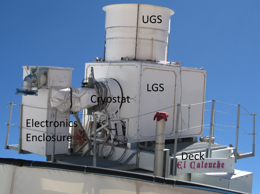
Figure 1.2: The QUIET instrument deployed to the Chajnantor Plateau in Chile’s Atacama Desert to reduce atmospheric emission.

This thesis contains the following elements. Chapter 1 introduces QUIET. Chapter 2 describes the electronics system. Chapter 3 describes data-management software and practices. Chapter LABEL:sec:observations describes the W-band observation from Chile. Chapter LABEL:sec:analysis describes the data analysis. Chapter LABEL:sec:results describes the results and my conclusions.

1.3.1   Module Operation Principles

The QUIET module implemented our polarization-detection scheme. Here I outline the module operation; §1.3.3 gives implementation details. The following discussion applies to an “ideal” module—one with no systematic errors. colin_thesis; quiet_instrument; and §1.3.3 of this thesis describe module non-idealities. The module was a pseudo-correlation polarimeter (gaier:296): the polarization signal appeared as the product of two independently-processed polarization states (Figure 1.3). The module operated entirely at radio frequency (RF). There was no intermediate frequency or local oscillator. The final stage of the module rectified and integrated the signal.

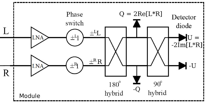
Figure 1.3: The QUIET module converted $L$ and $R$ into measurements of $Q$ and $U$. We modulated each measurement twice: once with each phase switch.

The module had two input ports. Normally, these received the left and right circular-polarization components ($L$ and $R$) of the CMB. Each input fed into a “leg” of the module. Each leg contained a phase switch that applied $0\mbox{${}^{\circ}$}$ or $180\mbox{${}^{\circ}$}$ phase shift to the incoming radiation. I denote the phase switch outputs by $\pm^{L}L$ and $\pm^{R}R$. The two legs then merged in a $180\mbox{${}^{\circ}$}$ hybrid coupler. The coupler output $\frac{\pm^{L}L\pm^{R}R}{\sqrt{2}}$ and $\frac{\pm^{L}L\mp^{R}R}{\sqrt{2}}$.

Detector diodes (Q1 and Q2) rectified half of each signal with resulting voltages

$$V_{\textrm{Q1}} \propto \frac{\pm^{L}L\pm^{R}R}{2}\frac{\pm^{L}L^{*}\pm^{R}R^{*}}{2}=\frac{LL^{*}\pm^{L}\pm^{R}(L^{*}R+LR^{*})+RR^{*}}{4}$$ (1.41)

$$= I/4\pm^{L}\pm^{R}\Re[L^{*}R]/2=\frac{I\pm^{L}\pm^{R}Q}{4}$$

$$V_{\textrm{Q2}} \propto \frac{\pm^{L}L\mp^{R}R}{2}\frac{\pm^{L}L^{*}\mp^{R}R^{*}}{2}=\frac{LL^{*}\pm^{L}\mp^{R}(L^{*}R+LR^{*})+RR^{*}}{4}$$ (1.42)

$$= \frac{I-\pm^{L}\pm^{R}Q}{4}$$

after using Eqs. 1.26 and 1.27. The other halves of the signal entered a second, $90\mbox{${}^{\circ}$}$ hybrid coupler which output $\frac{\pm^{L}L\mp^{R}R-i(\pm^{L}L\pm^{R}R)}{\sqrt{8}}$ and $\frac{\pm^{L}L\mp^{R}R+i(\pm^{L}L\pm^{R}R)}{\sqrt{8}}$. Two more detector diodes (U1 and U2) rectified these outputs with resulting voltages

$$V_{\textrm{U1}} \propto \frac{\pm^{L}L\mp^{R}R-i(\pm^{L}L\pm^{R}R)}{\sqrt{8}}\frac{\pm^{L}L^{*}\mp^{R}R^{*}+i(\pm^{L}L^{*}\pm^{R}R^{*})}{\sqrt{8}}$$ (1.43)

$$= \frac{1}{8}\left(LL^{*}-\pm^{L}\pm^{R}LR^{*}+iLL^{*}+\pm^{L}\pm^{R}iLR^{*}\right.$$

$$-\pm^{L}\pm^{R}RL^{*}+RR^{*}-\pm^{L}\pm^{R}iRL^{*}-iRR^{*}$$

$$-iLL^{*}+\pm^{L}\pm^{R}iLR^{*}+LL^{*}+\pm^{L}\pm^{R}LR^{*}$$

$$-\left.\pm^{L}\pm^{R}iRL^{*}+iRR^{*}+\pm^{L}\pm^{R}RL^{*}+RR^{*}\right)$$

$$= \frac{1}{8}\left(2LL^{*}+\pm^{L}\pm^{R}2iLR^{*}+2RR^{*}-\pm^{L}\pm^{R}2iRL^{*}\right)$$

$$= \frac{I-\pm^{L}\pm^{R}2\Re[iL^{*}R]}{4}=\frac{I-\pm^{L}\pm^{R}2\Im[L^{*}R]}{4}$$

$$= \frac{I-\pm^{L}\pm^{R}U}{4}$$

$$V_{\textrm{U2}} \propto \frac{\pm^{L}L\mp^{R}R+i(\pm^{L}L\pm^{R}R)}{\sqrt{8}}\frac{\pm^{L}L^{*}\mp^{R}R^{*}-i(\pm^{L}L^{*}\pm^{R}R^{*})}{\sqrt{8}}$$ (1.44)

$$= \frac{1}{8}\left(LL^{*}-\pm^{L}\pm^{R}LR^{*}-iLL^{*}-\pm^{L}\pm^{R}iLR^{*}\right.$$

$$-\pm^{L}\pm^{R}RL^{*}+RR^{*}+\pm^{L}\pm^{R}iRL^{*}+iRR^{*}$$

$$+iLL^{*}-\pm^{L}\pm^{R}iLR^{*}+LL^{*}+\pm^{L}\pm^{R}LR^{*}$$

$$+\left.\pm^{L}\pm^{R}iRL^{*}-iRR^{*}+\pm^{L}\pm^{R}RL^{*}+RR^{*}\right)$$

$$= \frac{1}{8}\left(2LL^{*}-\pm^{L}\pm^{R}2iLR^{*}+2RR^{*}+\pm^{L}\pm^{R}2iRL^{*}\right)$$

$$= \frac{I\pm^{L}\pm^{R}2\Re[iL^{*}R]}{4}=\frac{I-\pm^{L}\pm^{R}2\Im[L^{*}R]}{4}$$

$$= \frac{I\pm^{L}\pm^{R}U}{4}$$

after using Eqs. 1.26 and 1.28.

The electronics (§2) modulated the $L$ phase switch at 4 kHz and the $R$ phase switch at 50 Hz. After digitization we recorded the average (“TP”) and demodulation (“DE”) of the data in both 4-kHz phase switch states. For the Q1 diode these are

TP $$\propto (I\pm^{L}\pm^{R}Q)+(I\mp^{L}\pm^{R}Q)\propto I$$ (1.45)

DE $$\propto (I\pm^{L}\pm^{R}Q)-(I\mp^{L}\pm^{R}Q)\propto\pm^{R}Q.$$ (1.46)

We stored the data at 100 Hz so adjacent data samples had opposite signs of $\pm^{R}$. By subsequently differencing two adjacent samples we obtained “double-demodulated” (DD) data $\propto Q$. (The Q2 diode yielded the same except with $Q\rightarrow-Q$. The U diodes yielded the same except $Q\rightarrow U$.) Double demodulation reduced the effect of amplifier gain variations (1/f noise) and eliminated instrumental polarization otherwise caused by gain mismatch between the two legs (quiet_instrument). Furthermore each module (and therefore each pixel) fully characterized the linear polarization.

1.3.2   Optics

Our optical system consisted of the telescope, ground screen, feed horns, and septum polarizers. We chose a 1.4-m side-fed Dragonian antenna for the telescope. A comoving, absorbing ground screen limited the sidelobes. We used corrugated feed horns to form the beams for each module. Each feed horn sent its radiation to a septum polarizer, which separated $L$ and $R$ into different waveguides for the module.

The telescope used a two-reflector design (quiet_telescope) that satisfied the Mizuguchi condition (mizugutch). The result had a wide field of view (Figure 1.4), low instrumental polarization, and low sidelobes. We made the two mirrors out of aluminum, the backs of which we light-weighted and connected by hexapods with adjustable turnbuckles to a steel support structure. This support structure attached the telescope (and the remainder of the instrument) to the existing Cosmic Background Imager (CBI) mount (cbi_instrument). The mount had three rotation axes (azimuth, elevation, and “deck”). The azimuth axis was capable of fast scanning ($\approx 5\mbox{${}^{\circ}$}/$s) so that the typical scan frequency was well above the typical 1/f knee frequency. By regularly (§LABEL:sec:obs:cmb) rotating the third axis (deck), we modulated the instrumental-polarization axis, thereby suppressing instrumental polarization.

Figure 1.4: The module array had a large ($8\mbox{${}^{\circ}$}$) field of view on the sky. Each circle represents one module beam with diameter equal to the FWHM of $11\mbox{$.\mkern-4.0mu^{\prime}$}66$. The modules and their corresponding positions are labeled RQ0–RQ90. Modules RQ7, 8, 28, and 42 did not function. Modules RQ3 and RQ70 did not have any data passing selection. There was no module at position RQ81.

We enclosed the optics with a comoving, ambient-temperature, absorbing ground screen. The ground screen had two main parts: lower (LGS) and upper (UGS). The LGS was an aluminum box surrounding the mirrors with a hole for the cryostat. The UGS was a telescoping cylinder that surrounded the path of the main beam. Several smaller pieces formed the bottom ground screen (BGS) that covered the floor of the LGS and the gap between the LGS and the cryostat. We coated the entire inner surface of the ground screen with microwave absorber Emmerson Cummings HR-10 Eccosorb (ali_thesis). We sealed the Eccosorb with Volara (a microwave-transparent polyethylene foam) for weatherproofing. We coated the outer surface with white paint to minimize radiative loading.

Due to manufacturing delays, we did not install the UGS until January 2010. As a result, two significant sidelobes were present in the 2009 data. The “triple-reflection” sidelobe was due to a portion of the beam making an additional, unintended reflection off the secondary mirror. The result was a narrow ($1\mbox{${}^{\circ}$}$) sidelobe $50\mbox{${}^{\circ}$}$ away from the main beam (yuji_far_sidelobe). The “spillover” sidelobe resulted from part of the main beam escaping above the secondary mirror and LGS (Figure 1.5). The spillover appeared at $\approx 50\mbox{${}^{\circ}$}$ from the main beam in the opposite direction from the triple-reflection sidelobe; however, the spillover sidelobe was much more extended ($\pm 20\mbox{${}^{\circ}$}$ in the direction towards the main beam). Holes in the BGS caused additional spillover (sidelobe_measurement) (see also §LABEL:sec:noteworthy_events). We mitigated these effects with data selection (§LABEL:sec:cuts).

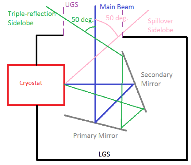
Figure 1.5: Before installation of the upper ground screen (in the middle of the observing season) two significant far sidelobes escaped the ground screen. The upper ground screen captured both sidelobes on a microwave absorber.

A corrugated, linear-flare feed horn formed the beam of each module. We constructed these feed horns as a hexagonally-close-packed “platelet array” (platelet).” We machined many large aluminum plates so that each plate formed a slice of all the feed horns, transverse to the optical axis. We then stacked the plates along the optical axis and diffusion bonded them together to form a single component containing all the feed horns. The platelet design incorporated light-weighting holes that also functioned as access holes for attachment screws. The fabrication costs of these arrays were at least an order of magnitude less than for the same number of electroformed feed horns. Measurements of the return loss and beam characteristics of the platelet arrays showed performance comparable to an equivalent electroformed design. The feed-horn full-width half-maximum (FWHM) was $7\mbox{$.\!\!^{\circ}$}0$–$8\mbox{$.\!\!^{\circ}$}6$ across the array, and instrumental polarization was $-29$ dB or better.

Radiation exited each feed horn into a septum polarizer (bornemann1995; omt_memo), which separated $L$ and $R$ for input to the QUIET detector modules. The polarizer itself was a square waveguide with a stepped-thickness septum in the center. The presence of the septum added a $90\mbox{${}^{\circ}$}$ phase shift to the TE₀₁ mode in the waveguide. A waveguide splitter followed the polarizer and physically separated the two outputs into rectangular WR-10 waveguides with spacing compatible with the module waveguide inputs. Although these waveguides carried components corresponding to circular polarization on the sky, the radiation in each waveguide was in a single, linearly-polarized (TE) mode. Polarizer imperfections caused temperature to polarization ($I\rightarrow Q/U$) leakage. Our lab measurements (omt_measurements) implied leakages of $\approx 0.3$%.

1.3.3   Modules

The QUIET detectors were miniaturized polarimeter modules (cleary:77412H) that converted $L$ and $R$ into $Q$ and $U$ as described in §1.3.1.” Each module was based on HEMT amplifiers. Previous experiments including PIQUE (pique2001), DASI (Leitch02), CBI (cbi_instrument), WMAP (jarosik2003), and CAPMAP (capmap_instrument) also used HEMT-based polarimeters, but we used advances in millimeter-wave circuit technology and packaging (Gaier20031167) to replace waveguide-block components and connections with strip-line–coupled devices. The resulting modules were 3.2 cm $\times$ 2.9 cm (Figure 1.6), almost an order of magnitude smaller than a comparable waveguide design. Each module had two waveguide inputs matched to the two septum-polarizer outputs. A probe in each port coupled the radiation into (50-$\Omega$) microstrip transmission lines. The first active component in each leg was a HEMT-based monolithic-microwave-integrated-circuit (MMIC) amplifier. A second MMIC provided additional amplification before the phase switch. After the phase switch, the signal passed through a bandpass filter before the third (final) MMIC. After the final MMIC, the two legs combined in the hybrid coupler. (For conceptual simplicity, §1.3.1 separates the hybrid coupler into a first $180\mbox{${}^{\circ}$}$ coupler and second $90\mbox{${}^{\circ}$}$ coupler. We manufactured both couplers as a single six-port device.) Each coupler output (Q1, Q2, U1, and U2) passed through a second bandpass filter before rectification at its detector diode.

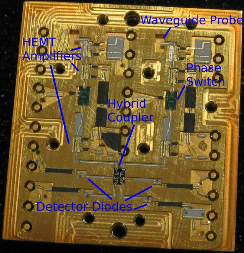
Figure 1.6: The QUIET module was a miniaturized correlation polarimeter. We used microstrip transmission lines to couple different components. This reduced the size by a factor of 10 compared to a traditional waveguide-based design.

The MMICs were low-noise amplifiers with four HEMT stages manufactured in an Indium-Phosphide (InP) process (module_doc). Each MMIC provided $\approx 25$ dB gain with noise temperature 50–80 K when cooled to a physical temperature of 20 K. At 20 K the MMICs required $\approx$ 10 mA of drain current bias, 0.5 V drain voltage, and 0.1 V gate voltage for optimum performance. Because the number of module electrical connections was limited, we connected MMIC drains together so that each leg had three gate connections and two drain connections. Thus each module had 10 MMIC bias connections in total. We optimized the sensitivity over these 10 parameters with a sparse–wire-grid calibration source (ltd_wiregrid) and downhill-simplex algorithm.

The phase switches were two-path circuits also fabricated in InP. One of the paths had an additional half-wavelength length so that radiation passing through it acquired a $180\mbox{${}^{\circ}$}$ phase shift. A PiN (p-type, intrinsic, n-type) diode controlled whether radiation could pass through each path. Reverse biasing the diode put it into a high-impedance state, blocking that path. When forward biased to 400 $\mu$A, the transmission was $\approx$ unity (Figure 2.6). Typically we forward biased one diode and reverse biased the other so the phase shift was either $0\mbox{${}^{\circ}$}$ or $180\mbox{${}^{\circ}$}$ as described in §1.3.1. However, we periodically (§LABEL:sec:regular_observations) made a diagnostic “offset” measurement by reverse biasing both diodes to block all RF power. Since each module had two phase switches and each switch had two diodes, there were four phase switch bias currents per module. Differences in transmission between the two paths would cause $I\rightarrow Q/U$ leakage if we did not use double demodulation. Because we used double demodulation, we did not attempt to balance the transmission by adjusting the diode biasing.

The hybrid coupler was a passive, planar InP device that summed its two inputs with either $0\mbox{${}^{\circ}$}$, $90\mbox{${}^{\circ}$}$, or $180\mbox{${}^{\circ}$}$ phase shifts as described in §1.3.1. Our design used Lange couplers and Schiffman phase delay lines to perform these functions (module_doc). Because the phase shifts were not exactly $90\mbox{${}^{\circ}$}$ or $180\mbox{${}^{\circ}$}$, the detector angles were different from their ideal values (sugarbaker_supp), and the noise correlations among the diodes also changed from their ideal values (white_noise_correlation).

The detector diodes were Schottky diodes (Agilent HSCH-9161) which we operated in the square-law regime. At 20 K the diodes required bias ($\approx 30$ $\mu$A) to make the impedance reasonable ($200\,\Omega$). The diode bias and readout was differential so each diode required two connections for a total of eight diode connections per module.

A brass housing contained the components of each module. Inside the housing, microstrip transmission lines connected the RF components. Ribbon bonds connected DC bias and readout points to pins leading out of the module. Each module had 23 such pins: 10 MMIC, 4 phase switch, 8 diode, and 1 shared module ground. Since all external module connections were DC, the modules were easy to test and optimize in a repeatable way.

1.3.4   Cryostat

The cryostat mounted and supported the platelet array, septum polarizers, and modules (Figure 1.7). Radiation entered the cryostat through an ultra-high–molecular-weight—polyethylene window with an expanded-Teflon anti-reflection coating. With this coating the loss through the window was at the percent level (The loss increased the system noise temperature by 4 K.) for microwave frequencies. A polystyrene filter blocked infrared radiation, reducing thermal loading on the cold stage. We made an interface plate in the cold stage between the platelet array and septum polarizers; the interface plate included waveguide transitions between the circular waveguide at the end of each feed horn and the square waveguide at the input of each septum polarizer. We cooled the cold stage containing the modules and optical components to $\approx$ 25 K using two CTI Cryogenics Cryodyne 1020 Gifford-McMahon refrigerators. We attached a heater to each cold head, and a temperature controller (Cryo-con model 32B, hereafter “CPID”) regulated the cold-head temperatures using a feedback loop. We put silicon diode thermometers on the detectors, platelet array, refrigerator heads, and secondary 80-K stage (The CTI 1020 has two cold stages. The 80-K stage cooled a radiation shield.) to continuously monitor the cooling and temperature regulation performance. The refrigerators had a mechanical cycle frequency of 1.2 Hz. I found a response at this frequency in the DD data (§LABEL:sec:cuts:ps_spikes). Stycast-epoxy–sealed hermetic pass-throughs allowed the bias and readout connections (§2.1) to be brought out of the cryostat.

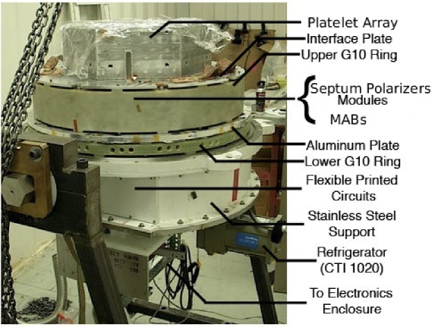
Figure 1.7: The cryostat contained the platelet array, septum polarizers, and modules. We cooled them to $\approx 25$ K to reduce the system noise.

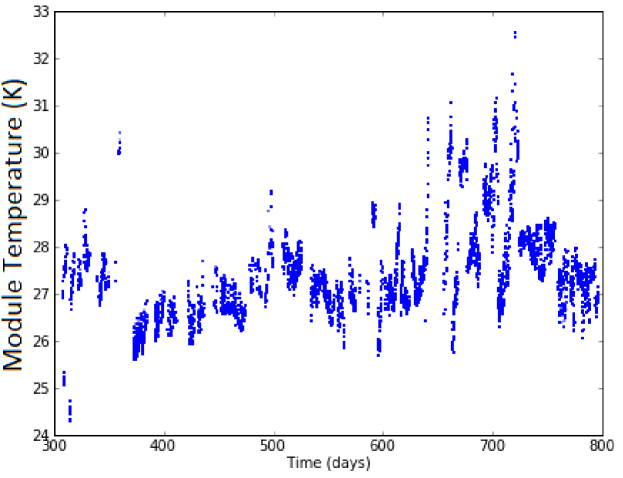
Figure 1.8: The cryostat temperature varied throughout the season due to problems with the cold heads and vacuum. The main effect was that the responsivity changed; we took it into account in the responsivity model and associated systematic error. (I show the temperature of the central module, RQ45.)

Chapter 2 Electronics

They said it couldn’t be done, but sometimes it doesn’t work out that way.

Casey Stengel

The electronics system provided module biasing, timing synchronization, and data acquisition (DAQ) for the receiver. We divided and assigned these tasks to four systems (Figure 2.1): (1) Passive Interfaces, (2) Bias, (3) Readout, and (4) Data Management. The Passive Interfaces system (§2.1) created an interface between the modules, the biasing electronics, and the DAQ. The Bias system (§2.2) generated the voltage or current necessary to operate each module active component. The Readout system (§2.3) amplified and digitized the module outputs. It included the timing synchronization hardware. The Data Management system (§3) commanded the other systems and recorded the data.

Figure 2.1: We divided the electronics into four systems: Passive Interfaces, Bias, Readout, and Data Management. Commands flowed from the observers, through the Bias and Passive Interfaces systems, and to the modules. The module outputs flowed through the Passive Interfaces system to the Readout system, which digitized them, and the Data Management system, which recorded them.

2.1 Passive Interfaces

The main function of the Passive Interfaces system was to bring the module electrical connections out of the cryostat. We accomplished this function in three stages: first, Module Assembly Boards (MAB) connected directly to the modules. Second, Flexible Printed Circuits (FPC) connected to the MABs and passed through the cryostat vacuum seal. Third, Array Interface Boards (AIB) interfaced between the FPCs and standard ribbon cables.

Each MAB was a printed circuit board with pin sockets for seven modules. (Sometimes “MAB” refers to the associated modules e.g. “MAB3 has high noise.”) We made five electrically identical MAB designs with different physical shapes as needed to fill the focal plane (Figure 2.2); there were 13 MABs in total. Each module had 27 pins (see §1.3.3 for their functions; four pins were unused). Voltage clamps and RC low-pass filters on the MAB protected the sensitive components inside the modules from damage caused by transients or accidental overvoltage. After protection, the MAB circuitry connected the (23 used) module pins to 40-contact Hirose connectors. Each MAB had 5 such connectors: 2 for MMIC bias pins, 2 for detector diodes, and 1 for phase switches. Each Hirose connector accepted one FPC.

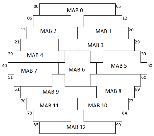
Figure 2.2: We tiled 13 MABs to fill the focal plane. Numbers to the left and right indicate module position numbers. MABs 0 and 3 had the same shape and were physically identical circuit boards. Similarly, MABs 1, 2, 4, and 5; 7, 8, 10, and 11; and 9 and 12 were physically identical. Thus we needed only five MAB circuit layouts. The modules could not rotate $180\mbox{${}^{\circ}$}$ in the focal plane so a duplicate MAB 4 cannot serve in place of MAB 7, for example.

The FPCs were high-density (40 conductors each) 32”-long flexible circuit boards. One end of each FPC connected to an MAB. Each FPC carried either MMIC, diode, or phase-switch signals for that MAB. We grouped the five FPCs for each MAB together for cable routing (there were $5\times 13=65$ FPCs in total). We clamped each FPC group to the cryostat 80-K stage to reduce thermal loading. Each FPC group passed through the cryostat wall in a Stycast-epoxy–filled custom hermetic seal. The other end of each FPC connected to an AIB.

The AIBs provided a second layer of electrical protection for the modules. We attached them to the back of the cryostat (Figure 2.3). When cold, the diodes comprising the voltage clamps on the MABs had drastically different I-V curves than when warm and were no longer effective at protecting the modules. (The filter resistances and capacitances could change as well.) Therefore, we duplicated the module protection circuitry on the AIBs. Each AIB accepted only MMIC, diode, or phase-switch FPCs. A MMIC AIB accepted four MMIC FPCs (from two MABs) and combined and routed the signals (after protection) to one AIB Cable (Harting) connector. The AIB Cables connected the AIBs to the bias boards (§2.2). We made each AIB Cable from two 80-pin shielded ribbon cables; AIB Cable Boards (Figure 2.4, see also AIB_cable_proposal) interfaced between the Harting connectors and the ribbon cables. A “Preamp” AIB (corresponding to “Preamp Boards,” §2.2) accepted four diode FPCs (from two MABs), and a Phase-switch AIB accepted three phase-switch FPCs (from three MABs). Each AIB connected one AIB Cable, which connected to one bias board (see Appendix LABEL:app:receiver_db_tables for the mapping between modules, MABs, and bias boards). We surrounded the AIBs and AIB Cable connections with a weatherproofing structure (Figure 2.5) to protect them from damage due to moisture and dust.

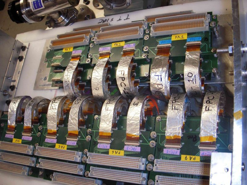
Figure 2.3: We attached the Array Interface Boards (AIB) to the back of the cryostat. Each AIB connected one bias board to two or three MABs. The AIBs also provided electrical protection for the modules. SOURCE: Alison Brizius

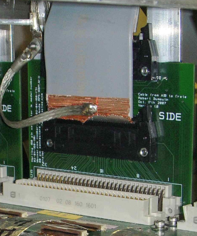
Figure 2.4: AIB Cable Boards interfaced between the Array Interface Board (AIB) Harting connectors (bottom) and the two ribbon cables making up each AIB Cable. SOURCE: Alison Brizius

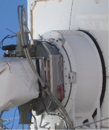
Figure 2.5: Weatherproofing protected the Array Interface Boards (AIB) and AIB Cable connections.

2.2 Bias

We made custom integrated-circuit boards to provide the bias signals needed to operate the modules. We apportioned the module components that require biasing to three types of bias boards: MMIC, Phase-switch, and Preamp. We monitored the biasing with a single Housekeeping Board. The boards communicated with other electronics systems through the Bias-Board Backplane. A weatherproof Electronics Enclosure housed and protected the Bias system (the Readout system shared this enclosure).

MMIC Boards provided voltage and current to power the MMIC amplifiers in the modules. Each MMIC Board could bias two MABs (14 modules); there were seven MMIC Boards in total. The boards provided voltage sources for the MMIC gates and drains. We stabilized each drain-voltage source with an op-amp feedback loop (mmic3_prototype). A 10-bit ($2^{10}$ settings) digital-to-analog converter (DAC) controlled each voltage. (The DACs were Linear Technologies LTC1660 chips. Each LTC1660 has eight independent DACs. We used an “address” 1–8 to distinguish different DACs on the same chip. The Preamp and Phase-switch Boards used the same chips. Unless otherwise noted, “DAC” means one of the DACs controlling a bias-board output.) Using a DAC to control each bias setting allowed us to reliably save and reapply the biasing state of the entire receiver. Moreover, with digital control we could optimize the performance upon adjusting the settings (§1.3.3).

Phase-switch Boards provided control to the PiN diodes in the module phase switches. Each Phase-switch Board could bias three MABs (21 modules); there were five Phase-switch Boards in total. For each phase switch, the Board forward biased one PiN diode and reverse biased the other diode. The reverse bias was always $-1.8$ V. We adjusted the forward bias (controlled by a DAC) to make the phase-switch transmission nearly independent of the bias setting (Figure 2.6 and §1.3.3). Because different diodes had different transmission in this plateau region, we could not balance the transmission between the two phase-switch states. Instead, we used double demodulation to remove the $I\rightarrow Q/U$ leakage that would otherwise be caused by the imbalance (quiet_instrument). At 4 kHz (50 Hz) the Phase-switch Board switched the bias direction of both diodes in the $L$ ($R$) phase switch. The Readout system provided synchronized clocks to synchronize the switching of the two switches. Because the AIB filtered the phase-switch bias, the switching transition was not instantaneous. We made the Readout system reject 17.5 $\mu$s of data during each transition when the signal was unstable (Figure 2.7).

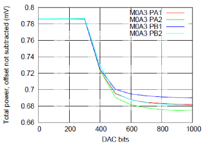
Figure 2.6: The phase-switch diodes required forward bias (positive DAC setting) to transmit power. Lower voltage corresponds to higher transmission power. The four phase-switch diodes (different colors) in each module had different transmission plateaus. We biased all phase-switch diodes in the plateau region and used double demodulation to remove the systematic effects of the transmission differences. SOURCE: ps_curve-20090117

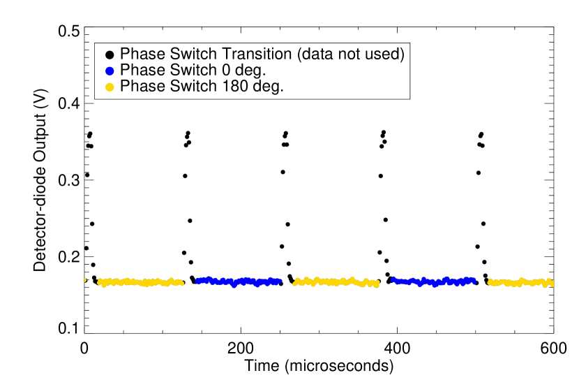
Figure 2.7: A phase switch modulated the sign of polarization at 4 kHz. We discarded the data during the phase-switch transition.

Preamp Boards biased and read out the detector diodes. Each Preamp Board could bias two MABs (14 modules); there were seven Preamp Boards in total. The bias circuit for each diode combined a floating current source with a differential voltage amplifier. A DAC controlled the bias current. The amplifier circuit subtracted a (DAC-adjustable) voltage offset so that the diode voltage, output by the Preamp Board, was centered in the dynamic range of the Readout system. §2.3 provides details about the amplification and filtering applied by the Preamp Board.

One Housekeeping Board monitored all the MMIC and phase-switch biases. (We monitored the diode bias by recording the DAC settings and diode voltages.) We added several current sense resistors and voltage-probe points to each bias board. Multiplexers on the bias boards selected one of these measurements to send to the Housekeeping Board. The Housekeeping Board selected the measurement from one bias board or a thermometer (recording the temperature in the cryostat or Electronics Enclosure) to digitize with a 16-bit analog-digital converter (ADC). We monitored 1774 biases and temperatures (Appendix LABEL:app:receiver_db_tables), and the multiplexing rate was 500 Hz. Thus we measured each every 3.5 s. The multiplexing cycled only during phase-switch transitions (during which we already discarded the data) so the multiplexing transition did not affect the module signal. Analog opto-isolators separated the bias circuitry from the monitoring circuitry. The Readout and Data Management systems controlled this multiplexing.

The Bias-Board Backplane housed the bias boards and provided an interface to them. It was a modified VME (VERSAmodule Eurocard bus) 6U backplane with a partial metal enclosure that supported the bias boards (Figure 2.8). The backplane P2 (bottom) pins were straight-through and connected the AIB Cables to the bias boards (electronics_box). We connected the P1 (top) pins connect together so the bias boards could communicate. These pins provided a path for the bias boards to send a monitored voltage to the Housekeeping Board, a path for the housekeeping digital output to the Readout system, distribution of the housekeeping multiplex address, distribution of the phase-switch clocks, and digital control of the DACs. Table 2.1 lists the location of each board in the backplane.

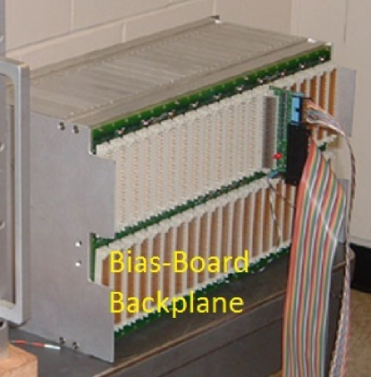
Figure 2.8: The bias boards entered through the face hidden in this photo. The AIB Cables connected to the lower set of connectors shown.

Table 2.1: Bias-board Locations

Slot	Board
1	Preamp 1
2	Preamp 2
3	Preamp 3
4	Preamp 4
5	Preamp 5
6	Preamp 6
7	Preamp 7
8	thermometer for Electronics Enclosure regulation
9	Housekeeping
10	MMIC 1
11	MMIC 2
12	MMIC 3
13	MMIC 4
14	MMIC 5
15	MMIC 6
16	MMIC 7
17	Phase-switch 1
18	Phase-switch 2
19	Phase-switch 3
20	Phase-switch 4
21	Phase-switch 5

The Electronics Enclosure housed and protected the Bias and Readout systems. It was an insulated 54”$\times$25”$\times$25” box we mounted next to the cryostat (DDB Unlimited OD-78DDXC, Figure 2.9 and §2.5.2 of ali_thesis). It contained the Bias-Board Backplane, power supplies, CPID, and Receiver PC (Personal Computer). Because the responsivity could vary with the electronics temperature, we regulated the temperature of the Electronics Enclosure.

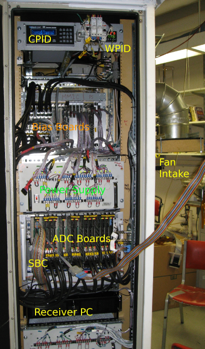
Figure 2.9: The Electronics Enclosure housed and protected the Bias and Readout systems.

2.2.1   Temperature Regulation

I designed a proportional-integral-derivative (PID) feedback-loop temperature-regulation system for the Electronics Enclosure (Figure 2.10 and enclosure_regulation_system). The system consisted of a PID controller (Omega CNi16D22-EI, denoted “WPID”), thermometer (McMaster-Carr 6577T35 resistance temperature detector), solid state relays (SSR, Carlo RJ1A23A20U), heater (McMaster-Carr 3575K13), and fan (McMaster-Carr 19135K95). I achieved good regulation performance ($<1\mbox{${}^{\circ}$}$C) on the time scale of a single observation (1 hour); however, the temperature changed significantly ($20\mbox{${}^{\circ}$}$C) throughout the season (§LABEL:sec:routine_checks:enclosure). I made a monitoring circuit to let the Data Management system record the heater and fan activity.

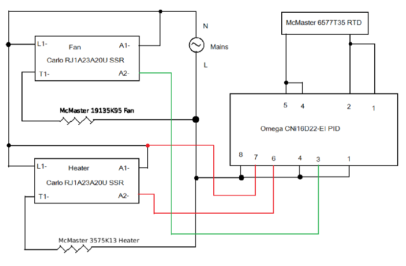
Figure 2.10: I made a proportional-integral-derivative (PID) system to regulate the Electronics Enclosure temperature. The numbers on the PID controller correspond to the physical numbered terminals. Wires of different colors do not connect except at filled circles. “L” represents the live electrical phase. When the PID turns on output 1, terminals 4 and 6 become connected. This connects the live phase to A2 on the Carlo SSR, activating the relay. The SSR connects L1 to T1, providing power to the heater. The same sequence applies to the fan (output 2) with terminals 1 and 3.

The WPID controlled the Enclosure temperature by alternately activating the heater or using the fan to bring cold air into the Enclosure. The thermometer measured the temperature in the Bias-Board Backplane. Based on this temperature, the WPID activated one of the outputs to bring the temperature to the setpoint ($35\mbox{${}^{\circ}$}$C or $40\mbox{${}^{\circ}$}$C depending on the time of year, see §LABEL:sec:routine_checks:enclosure). Each output activated an SSR that supplied power to the heater or fan. I mounted the heater directly above the Bias-Board Backplane; the heater supplied up to 1.1 kW. The fan brought cold ($-10$–$+15\mbox{${}^{\circ}$}$C) air in above the Bias-Board Backplane. Air circulation fans (McMaster-Carr 1985K11) kept the air inside the Enclosure well-mixed. The WPID had an ethernet interface, and I wrote a custom control program for remote control and automated operation by the Data Management system.

2.2.2   WPID Output Monitoring Board

The WPID did not report when it was turning on the fan and heater; therefore, I built an auxiliary monitoring circuit (“WPID Output Monitoring Board,” Figure 2.11). Linear power supplies converted convert the AC fan and heater voltages to 5 V DC. The WPID Output Monitoring Board supplied this voltage to the Receiver PC parallel port. A buffer (ON Semiconductor MC74VHC1GT125DT1G) and voltage divider (resistances 470 $\Omega$ and 560 $\Omega$) protected the port from overvoltage damage. I made the Data Management system sample the parallel-port input to record the heater and fan activity (§LABEL:sec:datacompilation).

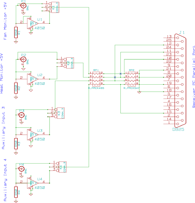
Figure 2.11: The WPID Output Monitoring Board sent the WPID heater and fan activity to the Data Management system for recording.

2.3 Readout

The Readout system amplified, filtered, and demodulated the signal. Preamp Boards provided analog amplification and low-pass filtering. ADC Boards digitized the module signals and demodulated them synchronously with the phase switching. A Time-code Reader provided the time and reference clocks for all electronics systems.

We used the Preamp Boards to measure the detector-diode voltage. Three analog amplifiers provided a gain of $\approx 130$. This amplifier chain contained low-pass filtering with three poles at 3-dB frequencies of 160 kHz, 340 kHz, and 32 MHz. This filtering prevented aliasing with the 800-kHz digitization sampling. As described in §2.2, the board subtracted a voltage offset to compensate for the diode-bias voltage. The Preamp Board output stage sent the amplified, filtered voltage to ADC Boards using one pair of wires (differential signaling) per diode.

ADC Boards digitized the diode voltages. Each ADC Board had 32 channels; however, we left four channels unused so each board digitized 28 diodes (seven modules, one MAB). Each channel had a low-pass filter (3 dB at 600 kHz) before digitization by 18-bit Analog Devices AD7674 Successive Approximation Register ADCs. The ADCs sampled at 800 kHz. Each ADC Board had a field-programmable gate array (FPGA), which accumulated the samples from the 32 ADCs on that Board. The FPGA on one ADC Board, designated the “Master ADC Board,””generated the 4-kHz and 50-Hz signals used by the Bias system to control the phase-switch modulation. We distributed these signals to all ADC Boards, and the FPGA on each ADC Board used them to demodulate the detector-diode signals synchronously with the phase-switch modulation.

Normally we recorded three 100-Hz data streams for each diode. We recorded short (1024-sample) “snapshots” of 800-kHz data for diagnostic and monitoring purposes; however, there was insufficient storage to record at that rate continuously. To create the TP data stream (§1.3.1), the FPGA summed all 800-kHz samples, regardless of phase-switch modulation. The TP stream was sensitive to Stokes $I$, and we used it for calibration and monitoring. To create the DE data stream, the FPGA differenced samples, assigning different signs to the two 4-kHz phase-switch states. We differenced two adjacent DE samples in post-processing to demodulate the 50-Hz phase state switching and create the DD stream. In the “quadrature” stream, we differenced 4-kHz samples $90\mbox{${}^{\circ}$}$ out of phase with the 4-kHz switching (Figure 2.12). The quadrature data had the same noise as DE data and no signal. We used quadrature data to monitor potential contamination and understand the detector noise properties. The three streams (TP, DE, and quadrature) together constituted the “radiometer data.” As mentioned in §2.2, the FPGA did not accumulate data in any stream when the phase-switch state was changing. This blanking rejected 14 out of every 100 samples, reducing the effective integration time.

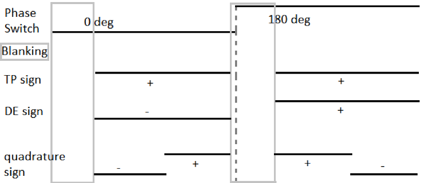
Figure 2.12: We implemented digital demodulation on the ADC Boards. We discarded data during phase-switch transitions (“Blanking”). The TP stream summed all data regardless of the phase-switch state. The DE stream differenced data between the (two 4-kHz) phase-switch states. Quadrature data was $90\mbox{${}^{\circ}$}$ out of phase so that we canceled the signal. (I exaggerated the fraction of data blanked, 14%, for ease of viewing.)

The ADC Boards had a small differential non-linearity in their response. At intervals of 1024 bits, the ADC output had a jump discontinuity of size $<40$ bits (Figure 2.13). The size was negligible compared to the large 1/f noise in the TP data. However, the effect in DE data was not negligible. When the average 800-kHz voltage level was near a discontinuity, the voltage difference between the two phase-switch states caused the level to move across the discontinuity. This caused the discontinuity to be added to the DE data. The 800-kHz noise (much higher per sample than per 100-Hz sample) smeared out the discontinuity, reducing its amplitude but also increasing its width in bit space (the jump can occur whenever the signal level plus noise encounters the discontinuity). We called this effect “Type-B glitching.” We mitigated the effects by using the Preamp Board offsets to move the typical voltage levels away from the discontinuities. However, some effect remained, and I corrected for Type-B in analysis (§LABEL:sec:calibration:typeb).

Figure 2.13: Type-B glitches were jump discontinuities (differential non-linearity) in the ADC response. The jumps were evenly spaced every 1024 bits; however, the jump size and direction were different for different jumps. When the input was near a jump, the difference between the two phase-switch states caused the jump size to add to the DE data.

The ADC Backplane contained the ADC Boards, Time-code Reader, and a single-board computer (SBC, part of the Data Management system). The ADC Backplane was a Wiener Series 6000 VME crate; we put it in the Electronics Enclosure. The Master ADC Board used the VME interface to distribute the phase-switch control signals (and all other clock signals for synchronization) to the other ADC Boards.

The timing hardware consisted of a Time-code Reader and Auxiliary Timing Board (ATB). The Time-code Reader synchronized the electronics to an external Global Positioning System (GPS) derived time. The ATB distributed timing signals from the Time-code Reader to the Master ADC Board, which synchronized the other ADC Boards.

The Time-code Reader was a Symmetricom TTM635VME-OCXO (tcr_manual). We used an IRIG-B (Inter-range Instrumentation Group Mod B) amplitude-modulated time code from the GPS receiver in the control room (§LABEL:sec:observations:site) as the reference. From the time code we created synchronized 1-Hz and 10-MHz clock signals. The ATB distributed these clocks to the Master ADC Board, which used them to synchronize all the ADC Boards.

We made the ATB to convert logic levels between the Time-code Reader and Master ADC Board. The Time-code Reader output levels were TTL/CMOS, but the Master ADC Board could only receive low-voltage differential signals (LVDS). We designed a small circuit board to convert between them (Figure 2.14). The board used National Semiconductor DS90C031 LVDS Differential Line Drivers.

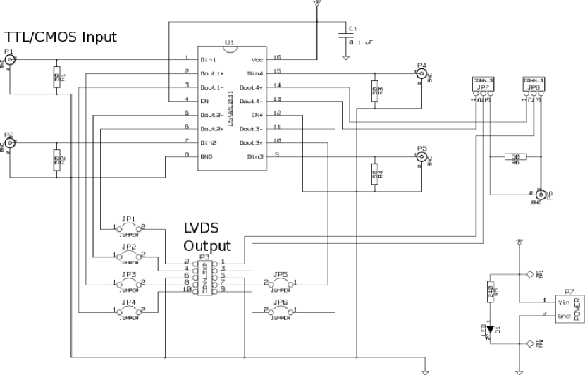
Figure 2.14: The Auxiliary Timing Board (ATB) converted logic levels between the Time-code Reader and Master ADC Board.

Chapter 3 Data Management

The first 90 percent of the code accounts for the first 90 percent of the development time. The remaining 10 percent of the code accounts for the other 90 percent of the development time.

Tom Cargill

The Data Management system was responsible for sending commands to the Bias system and mount pointing control system, receiving data from the Readout system, synchronizing data from different readout subsystems, and recording the data. We created several software processes that ran on several computers to accomplish these main functions. We organized the processes in a hierarchy. For example, the lowest level bias control process (adc_server) understands and implements only very simple commands e.g. “change the bias output of DAC #N to m bits.” Whereas the highest level control process (Receiver Control Panel) has a command “change the bias so the receiver is on.” Each process translated high level commands to low level commands (or low level data to high level data) appropriate for the other processes it communicated with. The subsections of this chapter detail these interactions.

We divided software processes into two broad categories: Online Software and Control Software. Online Software processes were always running and rarely used by the observers directly. Control Software processes had user-friendly graphical interfaces. The observers used them to schedule and start observations or monitor the system status. Two additional major Data Management components were the data files, whose format is described in §LABEL:sec:DAQ:files, and Receiver Database. The Receiver Database contained configuration information, e.g. which electronics board was connected to which module, which was used when translating command levels. Figure 3.1 is a simplified diagram of the Data Management system.

Figure 3.1: The Data Management system recorded, distributed, and stored the data. I wrote software processes that were its major components.

3.1 Online Software

The Online Software was responsible for the continuous readout and recording of the data. In addition, we periodically (or sporadically) generated bias commands. The Online Software translated these commands to the lowest level and sent them to electronics hardware. The Online Software helped us monitor the DAQ and command implementation status and automatically detected and reported several types of problems (Appendix LABEL:sec:DataCompilationStatusFlags) via the Control Software.

We created five processes to accomplish these functions. The adc_server ran on the single-board computer (SBC, a GE Fanuc VME-7700) in the ADC Backplane and was responsible for direct communication with electronics hardware or firmware. The DataCompilation process ran on the Receiver PC in the Electronics Enclosure and was responsible for combining data from different readout systems and distributing them to recording and monitoring processes. The ReceiverControl process ran on the Receiver PC and allowed us to enter high-level bias commands. The Bias Server process, which translated electronics bias commands, and PeripheralServer, which interfaced with auxiliary pressure sensors, temperature controllers, etc. are described in colin_thesis.

3.1.1   adc_server

The process adc_server was the lowest level of the Online Software. It communicated directly with the ADC Boards and Time-code Reader using the VME64 interface on the ADC Backplane. The process adc_server received commands from and sent data to higher-level Online Software processes via 100BaseTX ethernet (VMEPC_manual). The process adc_server was the only user process running on the SBC, and it ran continuously as long as the ADC Backplane was powered. I divided the functions among software threads. Since the SBC had only one Central Processing Unit (CPU) core, only one thread was running at any given time. The operating system (QUIET_DAQ_Crate) could switch rapidly between them, but some synchronization was necessary. Table LABEL:tab:adc_server:threads provides an overview of the threads and their functions.

lp3.5inp1.5in