Exploring Synchronization in Complex Oscillator Networks

Abstract

The emergence of synchronization in a network of coupled oscillators is a pervasive topic in various scientific disciplines ranging from biology, physics, and chemistry to social networks and engineering applications. A coupled oscillator network is characterized by a population of heterogeneous oscillators and a graph describing the interaction among the oscillators. These two ingredients give rise to a rich dynamic behavior that keeps on fascinating the scientific community. In this article, we present a tutorial introduction to coupled oscillator networks, we review the vast literature on theory and applications, and we present a collection of different synchronization notions, conditions, and analysis approaches. We focus on the canonical phase oscillator models occurring in countless real-world synchronization phenomena, and present their rich phenomenology. We review a set of applications relevant to control scientists. We explore different approaches to phase and frequency synchronization, and we present a collection of synchronization conditions and performance estimates. For all results we present self-contained proofs that illustrate a sample of different analysis methods in a tutorial style.

I Introduction

The scientific interest in synchronization of coupled oscillators can be traced back to the work by Christiaan Huygens on “an odd kind sympathy” between coupled pendulum clocks [1], and it still fascinates the scientific community nowadays [2, 3]. Within the rich modeling phenomenology on synchronization among coupled oscillators, we focus on the canonical model of a continuous-time limit-cycle oscillator network with continuous and bidirectional coupling.

A network of coupled phase oscillators: A mechanical analog of a coupled oscillator network is the spring network shown in Figure 1 and consists of a group of kinematic particles constrained to rotate around a circle and assumed to move without colliding.

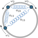
Figure 1: Mechanical analog of a coupled oscillator network

Each particle is characterized by a phase angle $\theta_{i}\in\mathbb{S}^{1}$ and has a preferred natural rotation frequency $\omega_{i}\in\mathbb{R}$. Pairs of interacting particles $i$ and $j$ are coupled through an elastic spring with stiffness $a_{ij}>0$. We refer to the Appendix -A for a first principle modeling of the spring-interconnected particles depicted in Figure 1.

Formally, each isolated particle is an oscillator with first-order dynamics $\dot{\theta}_{i}=\omega_{i}$. The interaction among $n$ such oscillators is modeled by a connected graph $G(\mathcal{V},\mathcal{E},A)$ with nodes $\mathcal{V}=\{1,\dots,n\}$, edges $\mathcal{E}\subset\mathcal{V}\times\mathcal{V}$, and positive weights $a_{ij}>0$ for each undirected edge $\{i,j\}\in\mathcal{E}$. Under these assumptions, the overall dynamics of the coupled oscillator network are

$$\dot{\theta}_{i}=\omega_{i}-\sum\nolimits_{j=1}^{n}a_{ij}\sin(\theta_{i}-\theta_{j})\,,\qquad i\in\{1,\dots,n\}\,.$$ (1)

The rich dynamic behavior of the coupled oscillator model (1) arises from a competition between each oscillator’s tendency to align with its natural frequency $\omega_{i}$ and the synchronization-enforcing coupling $a_{ij}\sin(\theta_{i}-\theta_{j})$ with its neighbors. Intuitively, a weakly coupled and strongly heterogeneous network does not display any coherent behavior, whereas a strongly coupled and sufficiently homogeneous network is amenable to synchronization, where all frequencies $\dot{\theta}_{i}(t)$ or even all phases $\theta_{i}(t)$ become aligned.

History, applications and related literature: The coupled oscillator model (1) has first been proposed by Arthur Winfree [4]. In the case of a complete interaction graph, the coupled oscillator dynamics (1) are nowadays known as the Kuramoto model of coupled oscillators due to Yoshiki Kuramoto [5, 6]. Stephen Strogatz provides an excellent historical account in [7]. We also recommend the survey [8].

Despite its apparent simplicity, the coupled oscillator model (1) gives rise to rich dynamic behavior. This model is encountered in various scientific disciplines ranging from natural sciences over engineering applications to social networks. The model and its variations appear in the study if biological synchronization phenomena such as pacemaker cells in the heart [9], circadian rhythms [10], neuroscience [11, 12, 13], metabolic synchrony in yeast cell populations [14], flashing fireflies [15], chirping crickets [16], biological locomotion [17], animal flocking behavior [18], fish schools [19], and rhythmic applause [20], among others. The coupled oscillator model (1) also appears in physics and chemistry in modeling and analysis of spin glass models [21, 22], flavor evolutions of neutrinos [23], coupled Josephson junctions [24], and in the analysis of chemical oscillations [25].

Some technological applications of the coupled oscillator model (1) include deep brain stimulation [26, 27], vehicle coordination [19, 28, 29, 30, 31], carrier synchronization without phase-locked loops [32], semiconductor lasers [33, 34], microwave oscillators [35], clock synchronization in decentralized computing networks [36, 37, 38, 39, 40, 41], decentralized maximum likelihood estimation [42], and droop-controlled inverters in microgrids [43]. Finally, the coupled oscillator model (1) also serves as the prototypical example for synchronization in complex networks [44, 45, 46, 47] and its linearization is the well-known consensus protocol studied in networked control, see the surveys and monographs [48, 49, 50]. Various control scientists explored the coupled oscillator model (1) as a nonlinear generalization of the consensus protocol [51, 52, 53, 54, 55, 56, 57].

Second-order variations of the coupled oscillator model (1) appear in synchronization phenomena, in population of flashing fireflies [58], in particle models mimicking animal flocking behavior [59, 60], in structure-preserving power system models, [61, 62] in network-reduced power system models [63, 64], in coupled metronomes [65], in pedestrian crowd synchrony on London’s Millennium bridge [66], and in Huygen’s pendulum coupled clocks [67]. Coupled oscillator networks with second-order dynamics have been theoretically analyzed in [68, 69, 70, 71, 72, 73, 8, 74], among others.

Coupled oscillator models of the form (1) are also studied from a purely theoretic perspective in the physics, dynamical systems, and control communities. At the heart of the coupled oscillator dynamics is the transition from incoherence to synchrony. Here, different notions and degrees of synchronization can be distinguished [74, 75, 76], and the (apparently) incoherent state features rich and largely unexplored dynamics as well [77, 78, 79, 47]. In this article we will be particularly interested in phase and frequency synchronization when all phases $\theta_{i}(t)$ become aligned, respectively all frequencies $\dot{\theta}_{i}(t)$ become aligned. We refer to [76, 64, 19, 80, 31, 81, 82, 53, 83, 52, 84, 85, 86, 87, 88, 89, 90, 75, 7, 8, 74, 56, 91, 92, 28, 93, 94, 95, 96, 97, 98, 99, 100, 101, 102, 103, 104, 105, 106, 107, 108, 95, 109, 110, 111, 112, 113, 114] for an incomplete overview concerning numerous recent research activities. We will review some of literature throughout the paper and refer to the surveys [8, 74, 7, 44, 45, 46] for further applications and numerous additional theoretic results concerning the coupled oscillator model (1).

Contributions and contents: In this paper, we introduce the reader to synchronization in networks of coupled oscillators. We present a sample of important analysis concepts in a tutorial style and from a control-theoretic perspective.

In Section II, we will review a set of selected technological applications which are directly tied to the coupled oscillator model (1) and also relevant to control systems. We will cover vehicle coordination, electric power networks, and clock synchronization in depth, and also justify the importance of the coupled oscillator model (1) as a canonical model. Prompted by these applications, we review the existing results concerning phase synchronization, phase balancing, and frequency synchronization, and we also present some novel results on synchronization in sparsely-coupled networks.

In particular, Section III introduces the reader to different synchronization notions, performance metrics, and synchronization conditions. We illustrate these results with a simple yet rich example that nicely explains the basic phenomenology in coupled oscillator networks.

Section IV presents a collection of important results regarding phase synchronization, phase balancing, and frequency synchronization. By now the analysis methods for synchronization have reached a mature level, and we present simple and self-contained proofs using a sample of different analysis methods. In particular, we present one result on phase synchronization and one result on phase balancing including estimates on the exponential synchronization rate and the region of attraction (see Theorem IV.3 and Theorem IV.4). We also present some implicit and explicit, and necessary and sufficient conditions for frequency synchronization in the classic homogeneous case of a complete and uniformly-weighted coupling graphs (see Theorem IV.5). Concerning frequency synchronization in sparse graphs, we present two partially new synchronization conditions depending on the algebraic connectivity (see Theorem IV.6 and Theorem IV.7).

In our technical presentation, we try to strike a balance between mathematical precision and removing unnecessary technicalities. For this reason some proofs are reported in the appendix and others are only sketched here with references to the detailed proofs elsewhere. Hence, the main technical ideas are conveyed while the tutorial value is maintained.

Finally, Section V concludes the paper. We summarize the limitations of existing analysis methods and suggest some important directions for future research.

Preliminaries and notation: The remainder of this section introduces some notation and recalls some preliminaries.

Vectors and functions: Let $\mathbf{1}_{n}$ and $\mathbf{0}_{n}$ be the $n$-dimensional vector of unit and zero entries, and let $\mathbf{1}_{n}^{\perp}$ be the orthogonal complement of $\mathbf{1}_{n}$ in $\mathbb{R}^{n}$, that is, $\mathbf{1}_{n}^{\perp}\triangleq\{x\in\mathbb{R}^{n}:\,x\perp\mathbf{1}_{n}\}$. Given an $n$-tuple $(x_{1},\dots,x_{n})$, let $x\in\mathbb{R}^{n}$ be the associated vector with maximum and minimum elements $x_{\textup{max}}$ and $x_{\textup{min}}$. For an ordered index set $\mathcal{I}$ of cardinality $|\mathcal{I}|$ and an one-dimensional array $\{x_{i}\}_{i\in\mathcal{I}}$, let $\operatorname*{\mathrm{diag}}(\{c_{i}\}_{i\in\mathcal{I}})\in\mathbb{R}^{|\mathcal{I}|\times|\mathcal{I}|}$ be the associated diagonal matrix. Finally, define the continuous function $\operatorname*{sinc}:\mathbb{R}\rightarrow\mathbb{R}$ by $\operatorname*{sinc}(x)=\sin(x)/x$ for $x\neq 0$.

Geometry on the $n$-torus: The set $\mathbb{S}^{1}$ denotes the unit circle, an angle is a point $\theta\in\mathbb{S}^{1}$, and an arc is a connected subset of $\mathbb{S}^{1}$. The geodesic distance between two angles $\theta_{1}$, $\theta_{2}\in\mathbb{S}^{1}$ is the minimum of the counter-clockwise and the clockwise arc lengths connecting $\theta_{1}$ and $\theta_{2}$. With slight abuse of notation, let $|\theta_{1}-\theta_{2}|$ denote the geodesic distance between two angles $\theta_{1},\theta_{2}\in\mathbb{S}^{1}$. The $n$-torus is the product set $\mathbb{T}^{n}=\mathbb{S}^{1}\times\dots\times\mathbb{S}^{1}$ is the direct sum of $n$ unit circles. For $\gamma\in{[0,2\pi[}$, let $\overline{\mbox{Arc}}_{n}(\gamma)\subset\mathbb{T}^{n}$ be the closed set of angle arrays $\theta=(\theta_{1},\dots,\theta_{n})$ with the property that there exists an arc of length $\gamma$ containing all $\theta_{1},\dots,\theta_{n}$. Thus, an angle array $\theta\in\overline{\mbox{Arc}}_{n}(\gamma)$ satisfies $\max\nolimits_{i,j\in\{1,\dots,n\}}|\theta_{i}-\theta_{j}|\leq\gamma$. Finally, let $\mbox{Arc}_{n}(\gamma)$ be the interior of the set $\overline{\mbox{Arc}}_{n}(\gamma)$.

Algebraic graph theory: Let $G(\mathcal{V},\mathcal{E},A)$ be an undirected, connected, and weighted graph without self-loops. Let $A\in\mathbb{R}^{n\times n}$ be its symmetric nonnegative adjacency matrix with zero diagonal, $a_{ii}=0$. For each node $i\in\{1,\dots,n\}$, define the nodal degree by $\textup{deg}_{i}=\sum\nolimits_{j=1}^{n}a_{ij}$. Let $L\in\mathbb{R}^{n\times n}$ be the Laplacian matrix defined by $L=\operatorname*{\mathrm{diag}}(\{\textup{deg}_{i}\}_{i=1}^{n})-A$. If a number $\ell\in\{1,\dots,|\mathcal{E}|\}$ and an arbitrary direction is assigned to each edge $\{i,j\}\in\mathcal{E}$, the (oriented) incidence matrix $B\in\mathbb{R}^{n\times|\mathcal{E}|}$ is defined component-wise by $B_{k\ell}=1$ if node $k$ is the sink node of edge ${\ell}$ and by $B_{k\ell}=-1$ if node $k$ is the source node of edge ${\ell}$; all other elements are zero. For $x\in\mathbb{R}^{n}$, the vector $B^{T}x$ has components $x_{i}-x_{j}$ corresponding to the oriented edge from $j$ to $i$, that is, $B^{T}$ maps node variables $x_{i}$, $x_{j}$ to incremental edge variables $x_{i}-x_{j}$. If $\operatorname*{\mathrm{diag}}(\{a_{ij}\}_{\{i,j\}\in\mathcal{E}})$ is the diagonal matrix of edge weights, then $L=B\operatorname*{\mathrm{diag}}(\{a_{ij}\}_{\{i,j\}\in\mathcal{E}})B^{T}$. If the graph is connected, then $\mathrm{Ker\,}(B^{T})=\mathrm{Ker\,}(L)=\mathrm{span}(\mathbf{1}_{n})$, all $n-1$ non-zero eigenvalues of $L$ are strictly positive, and the second-smallest eigenvalue $\lambda_{2}(L)$ is called the algebraic connectivity and is a spectral connectivity measure.

II Applications of Kuramoto Oscillators Relevant to Control Systems

The mechanical analog in Figure 1 provides an intuitive illustration of the coupled oscillator dynamics (1), and we reviewed a wide range of examples from physics, life sciences, and technology in Section I. Here, we detail a set of selected technological applications which are relevant to control systems scientists.

II-A Flocking, Schooling, and Planar Vehicle Coordination

An emerging research field in control is the coordination of autonomous vehicles based on locally available information and inspired by biological flocking phenomena. Consider a set of $n$ particles in the plane $\mathbb{R}^{2}$, which we identify with the complex plane $\mathbb{C}$. Each particle $i\in\mathcal{V}=\{1,\dots,n\}$ is characterized by its position $r_{i}\in\mathbb{C}$, its heading angle $\theta_{i}\in\mathbb{S}^{1}$, and a steering control law $u_{i}(r,\theta)$ depending on the position and heading of itself and other vehicles. For simplicity, we assume that all particles have constant and unit speed. The particle kinematics are then given by [115]

$$\begin{split}\dot{r}_{i}&=e^{\textup{i}\theta_{i}}\,,\\ \dot{\theta}_{i}&=u_{i}(r,\theta)\,,\end{split}\qquad\Biggr{\}}\quad i\in\{1,\dots,n\}\,,$$ (2)

where $\textup{i}=\sqrt{-1}$ is the imaginary unit. If the control $u_{i}$ is identically zero, then particle $i$ travels in a straight line with orientation $\theta_{i}(0)$, and if $u_{i}=\omega_{i}\in\mathbb{R}$ is a nonzero constant, then the particle traverses a circle with radius $1/|\omega_{i}|$.

The interaction among the particles is modeled by a possibly time-varying interaction graph $G(\mathcal{V},\mathcal{E}(t),A(t))$ determined by communication and sensing patterns. Some interesting motion patterns emerge if the controllers use only relative phase information between neighboring particles, that is, $u_{i}=\omega_{0}(t)+f_{i}(\theta_{i}-\theta_{j})$ for $\{i,j\}\in\mathcal{E}(t)$ and $\omega_{0}:\,\mathbb{R}_{\geq 0}\to\mathbb{R}$. For example, the control $u_{i}=\omega_{0}(t)-K\cdot\sum_{j=1}^{n}a_{ij}(t)\sin(\theta_{i}-\theta_{j})$ with gain $K\in\mathbb{R}$ results in

$$\dot{\theta}_{i}=\omega_{0}(t)-K\cdot\sum\nolimits_{j=1}^{n}a_{ij}(t)\sin(\theta_{i}-\theta_{j})\,,\quad i\in\mathcal{V}\,.$$ (3)

The controlled phase dynamics (3) correspond to the coupled oscillator model (1) with a time-varying interaction graph with weights $K\cdot a_{ij}(t)$ and identically time-varying natural frequencies $\omega_{i}=\omega_{0}(t)$ for all $i\in\{1,\dots,n\}$. The controlled phase dynamics (3) give rise to very interesting coordination patterns that mimic animal flocking behavior [18] and fish schools [19]. Inspired by these biological phenomena, the controlled phase dynamics (3) and its variations have also been studied in the context of tracking and formation controllers in swarms of autonomous vehicles [19, 28, 29, 30, 31]. A few trajectories are illustrated in Figure 2, and we refer to [19, 28, 29, 30, 31] for other control laws and motion patterns.

In the following sections, we will present various tools to analyze the motion patterns in Figure 2, which we will refer to as phase synchronization and phase balancing.

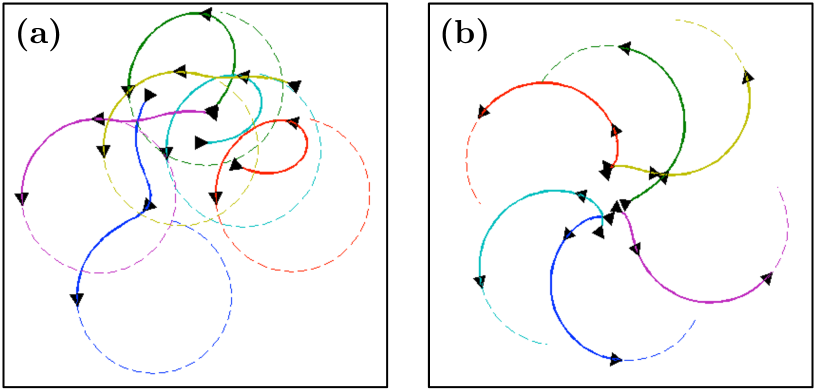
Figure 2: Illustration of the controlled dynamics (2)-(3) with $n\!=\!6$ particles, a complete interaction graph, and identical and constant natural frequencies $\omega_{0}(t)=1$, where $K\!=\!1$ in panel (a) and $K\!=\!-1$ in panel (b). The arrows depict the orientation, the dashed curves show the long-term position dynamics, and the solid curves show the initial transient position dynamics. It can be seen that even for this simple choice of controller, the resulting motion results in “synchronized” or “balanced” heading angles for $K=\pm 1$.

II-B Power Grids with Synchronous Generators and Inverters

Here, we present the structure-preserving power network model introduced in [61] and refer to [62, Chapter 7] for detailed derivation from a higher order first principle model. Additionally, we equip the power network model with a set of inverters and refer to [43] for a detailed modeling.

Consider an alternating current (AC) power network modeled as an undirected, connected, and weighted graph with node set $\mathcal{V}=\{1,\dots,n\}$, transmission lines $\mathcal{E}\subset\mathcal{V}\times\mathcal{V}$, and admittance matrix $Y\!=\!Y^{T}\in\mathbb{C}^{n\times n}$. For each node, consider the voltage phasor $V_{i}=|V_{i}|e^{\textup{i}\theta_{i}}$ corresponding to the phase $\theta_{i}\in\mathbb{S}^{1}$ and magnitude $|V_{i}|\geq 0$ of the sinusoidal solution to the circuit equations. If the network is lossless, then the active power flow from node $i$ to $j$ is $a_{ij}\sin(\theta_{i}-\theta_{j})$, where we used the shorthand $a_{ij}=|V_{i}|\cdot|V_{j}|\cdot\Im(Y_{ij})$.

In the following, we assume that the node set is partitioned as $\mathcal{V}=\mathcal{V}_{1}\operatorname{\cup}\mathcal{V}_{2}\operatorname{\cup}\mathcal{V}_{3}$, where $\mathcal{V}_{1}$ are load buses, $\mathcal{V}_{2}$ are conventional synchronous generators, and $\mathcal{V}_{3}$ are grid-connected direct current (DC) power sources, such as solar farms. The active power drawn by a load $i\in\mathcal{V}_{1}$ consists of a constant term $P_{\textup{l},i}>0$ and a frequency-dependent term $D_{i}\dot{\theta}_{i}$ with $D_{i}>0$. The resulting power balance equation is

$$D_{i}\dot{\theta}_{i}+P_{\textup{l},i}=-\sum\nolimits_{j=1}^{n}a_{ij}\sin(\theta_{i}-\theta_{j})\,,\;\;\;i\in\mathcal{V}_{1}\,.$$ (4)

If the generator reactances are absorbed into the admittance matrix, then the swing dynamics of generator $i\in\mathcal{V}_{2}$ are

$$M_{i}\ddot{\theta}_{i}+D_{i}\dot{\theta}_{i}=P_{\textup{m},i}-\sum\nolimits_{j=1}^{n}a_{ij}\sin(\theta_{i}-\theta_{j})\,,\;\;\;i\in\mathcal{V}_{2},$$ (5)

where $\theta_{i}\in\mathbb{S}^{1}$ and $\dot{\theta}_{i}\in\mathbb{R}^{1}$ are the generator rotor angle and frequency, $P_{\textup{m},i}>0$ is the mechanical power input, and $M_{i}>0$, and $D_{i}>0$ are the inertia and damping coefficients.

We assume that each DC source is connected to the AC grid via an DC/AC inverter, the inverter output impendances are absorbed into the admittance matrix, and each inverter is equipped with a conventional droop-controller. For a droop-controlled inverter $i\in\mathcal{V}_{3}$ with droop-slope $1/D_{i}>0$, the deviation of the power output $\sum\nolimits_{j=1}^{n}a_{ij}\sin(\theta_{i}-\theta_{j})$ from its nominal value $P_{\textup{d},i}>0$ is proportional to the frequency deviation $D_{i}\dot{\theta}_{i}$. This gives rise to the inverter dynamics

$$D_{i}\dot{\theta}_{i}=P_{\textup{d},i}-\sum\nolimits_{j=1}^{n}a_{ij}\sin(\theta_{i}-\theta_{j})\,,\;\;\;i\in\mathcal{V}_{3}\,.$$ (6)

These power network devices are illustrated in Figure 3.

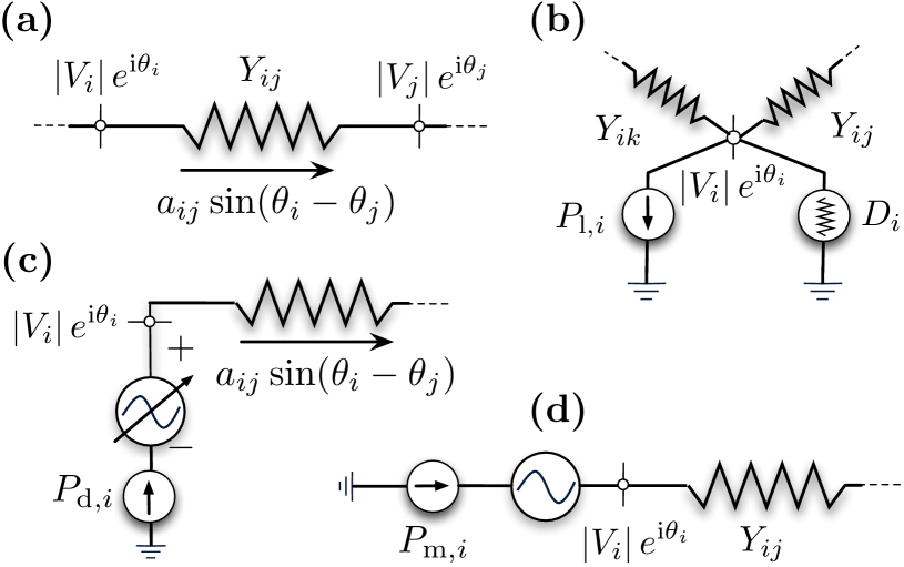
Figure 3: Illustration of the power network devices as circuit elements. Subfigure (a) shows a transmission element connecting nodes $i$ and $j$, Subfigure (b) shows a frequency-dependent load, Subfigure (c) shows an inverter controlled according to (6), and Subfigure (d) shows a synchronous generator.

Finally, we remark that different load models such as constant power/current/susceptance loads and synchronous motor loads can be modeled and analyzed by the same set of equations (4)-(6), see [62, 116, 117, 63, 64].

Synchronization is pervasive in the operation of power networks. All generating units of an interconnected grid must remain in strict frequency synchronism while continuously following demand and rejecting disturbances. Notice that, with exception of the inertial terms $M_{i}\ddot{\theta}_{i}$ and the possibly non-unit coefficients $D_{i}$, the power network dynamics (4)-(6) are a perfect electrical analog of the coupled oscillator model (1) with $\omega=(-P_{\textup{l},i},P_{\textup{m},i},P_{\textup{d},i})$. Thus, it is not surprising that scientists from different disciplines recently advocated coupled oscillator approaches to analyze synchronization in power networks [118, 119, 43, 120, 114, 64, 121, 122, 97, 69].

The theoretic tools presented in the following sections establish how frequency synchronization in power networks depend on the nodal parameters $(P_{\textup{l},i},P_{\textup{m},i},P_{\textup{d},i})$ as well as the interconnecting electrical network with weights $a_{ij}$. Ultimately, this deep understanding of synchrony gives us the correct intuition to design controllers and remedial action schemes preventing the loss of synchrony.

II-C Clock Synchronization in Decentralized Networks

Another emerging technological application of the coupled oscillator model (1) is clock synchronization in decentralized computing networks, such as wireless and distributed software networks. A natural approach to clock synchronization is to treat each clock as a coupled oscillator and follow a diffusion-based protocol to synchronize them, see the historic and recent surveys [36, 37], the landmark paper [38], and the interesting recent results [39, 40, 41].

Consider a set of distributed processors $\mathcal{V}=\{1,\dots,n\}$ interconnected in a (possibly directed) communication network. Each processor is equipped with an internal software clock, and these clocks need to be synchronized for distributed computing and network routing tasks. For simplicity, we consider only analog clocks with continuous coupling since digital clocks are essentially discretized analog clocks and pulse-coupled clocks can be modeled continuously after a phase reduction and averaging analysis.

For our purposes, the clock of processor $i$ is a voltage-controlled oscillator which outputs a harmonic waveform $s_{i}(t)=\sin(\theta_{i}(t))$, where $\theta_{i}(t)$ is the accumulated instantaneous phase. For uncoupled nodes, the phase $\theta_{i}(t)$ evolves as

$$\theta_{i}(t)=\left(\theta_{i}(0)+\frac{2\pi}{T_{\textup{nom}}+T_{i}}t\right)\textup{mod}(2\pi)\,,\quad i\in\{1,\dots,n\}\,.$$

where $T_{\textup{nom}}>0$ is the nominal period, $T_{i}\in\mathbb{R}$ is an offset (frequency offset or skew), and $\theta_{i}(0)\in\mathbb{S}^{1}$ is the initial phase. To synchronize their internal clocks, the processors follow a diffusion-based protocol. In a first step, neighboring oscillators continuously communicate their respective waveforms $s_{i}(t)$ to another. Second, through a phase detector each node measures a convex combination of phase differences as

$$\textup{cvx}_{i}(\theta(t))=\sum\nolimits_{j=1}^{n}a_{ij}f(\theta_{i}(t)-\theta_{j}(t))\,,\quad i\in\{1,\dots,n\}\,,$$

where $a_{ij}\!\geq\!0$ are convex ($\sum_{j=1}^{n}a_{ij}\!=\!1$) and detector-specific weights, and $f:\mathbb{S}^{1}\to\mathbb{R}$ is an odd $2\pi$-periodic function. Finally, $\textup{cvx}_{i}(\theta(t))$ is fed to a (first-order and constant) phase-locked loop filter $K$ whose output drives the local phase according to

$$\dot{\theta}_{i}(t)=\frac{2\pi}{T_{i}}+K\cdot\textup{cvx}_{i}(\theta(t))\,,\quad i\in\{1,\dots,n\}\,.$$ (7)

The goal of the synchronization protocol (7) is to synchronize the frequencies $\dot{\theta}_{i}(t)$ or even the phases $\theta_{i}(t)$ in the processor network. For an undirected communication protocol, symmetric weights $a_{ij}=a_{ji}$, and a sinusoidal coupling function $f(\cdot)=\sin(\cdot)$, the synchronization protocol (7) equals again the coupled oscillator model (1).

The tools developed in the next section will enable us to state conditions when the protocol (7) successfully achieves phase or frequency synchronization. Of course, the protocol (7) is merely a starting point, more sophisticated phase-locked loop filters can be constructed to enhance steady-state deviations from synchrony, and communication and phase noise as well as time-delays can be considered in the design.

II-D Canonical Coupled Oscillator Model

The importance of the coupled oscillator model (1) does not stem only from the various examples listed in Sections I and II. Even though model (1) appears to be quite specific (a phase oscillator with constant driving term and continuous, diffusive, and sinusoidal coupling), it is the canonical model of coupled limit-cycle oscillators [123]. In the following, we briefly sketch how such general models can be reduced to model (1). We schematically follow the approaches [124, Chapter 10],[125] developed in the computational neuroscience community without aiming at mathematical precision, and we refer to [123, 126] for further details.

Consider an oscillator modeled as a dynamical system with state $x\in\mathbb{R}^{m}$ and nonlinear dynamics $\dot{x}=f(x)$, which admit a locally exponentially stable periodic orbit $\gamma\subset\mathbb{R}^{m}$ with period $T>0$. By a change of variables, any trajectory in a local neighborhood of $\gamma$ can be characterized by a phase variable $\varphi\in\mathbb{S}^{1}$ with dynamics $\dot{\varphi}=\Omega$, where $\Omega=2\pi/T$.

Now consider a weakly forced oscillator of the form

$$\dot{x}=f(x)+\epsilon\cdot\delta(t)\,,$$ (8)

where $\epsilon>0$ is sufficiently small and $\delta(t)$ is a time-dependent forcing term. For small forcing $\epsilon\delta(t)$, the attractive limit cycle $\gamma$ persists, and the phase dynamics are obtained as

$$\dot{\varphi}=\Omega+\epsilon Q(\varphi)\delta(t)+\mathcal{O}(\epsilon^{2})\,,$$

where $Q(\varphi)$ is the infinitesimal phase response curve (or linear response function), and we dropped higher order terms.

Now consider $n$ such limit cycle oscillators, where $x_{i}\in\mathbb{R}^{m}$ is the state of oscillator $i$ with limit cycle $\gamma_{i}\subset\mathbb{R}^{m}$ and period $T_{i}>0$. We assume that the oscillators are weakly coupled with interaction graph $G(\mathcal{V},\mathcal{E})$ and dynamics

$$\dot{x}_{i}=f_{i}(x_{i})+\epsilon\sum\nolimits_{\{i,j\}\in\mathcal{E}}g_{ij}(x_{i},x_{j})\,,\;\;i\in\{1,\dots,n\}\,,$$ (9)

where $g_{ij}(\cdot)$ is the coupling function for the pair $\{i,j\}\in\mathcal{E}$. The coupling $g_{ij}(\cdot)$ can possibly be impulsive. The weak coupling in (9) can be identified with the weak forcing in (8), and a transformation to phase coordinates yields

$$\dot{\varphi}_{i}=\Omega_{i}+\epsilon\sum\nolimits_{\{i,j\}\in\mathcal{E}}Q_{i}(\varphi)g_{ij}(x_{i}(\varphi_{i}),x_{j}(\varphi_{j}))\,,$$

where $\Omega_{i}=2\pi/T_{i}$. The local change of variables $\theta_{i}(t)=\varphi_{i}(t)-\Omega_{i}t$ then yields the coupled phase dynamics

$$\dot{\theta}_{i}=\epsilon\sum\nolimits_{\{i,j\}\in\mathcal{E}}\!\!Q_{i}(\theta_{i}+\Omega_{i}t)g_{ij}(x_{i}(\theta_{i}+\Omega_{i}t),x_{j}(\theta_{j}+\Omega_{j}t)).$$

An averaging analysis applied to the $\theta$-dynamics results in

$$\dot{\theta}_{i}=\epsilon\omega_{i}+\epsilon\sum\nolimits_{\{i,j\}\in\mathcal{E}}h_{ij}(\theta_{i}-\theta_{j})\,,$$ (10)

where $\omega_{i}=h_{ii}(0)$ and the averaged coupling functions are

$$h_{ij}(\chi)=\lim_{T\to\infty}\frac{1}{T}\int_{0}^{T}\!Q_{i}(\Omega_{i}\tau)g_{ij}(x_{i}(\Omega_{i}\tau),x_{j}(\Omega_{j}\tau-\chi))d\tau.$$

Notice that the averaged coupling functions $h_{ij}$ are $2\pi$-periodic and the coupling is diffusive. If all functions $h_{ij}$ are odd, a first-order Fourier series expansion of $h_{ij}$ yields $h_{ij}(\cdot)\approx a_{ij}\sin(\cdot)$ as first harmonic with some coefficient $a_{ij}$. In this case, the dynamics (10) in the slow time scale $\tau=\epsilon t$ reduce exactly to the coupled oscillator model (1).

This analysis justifies calling the coupled oscillator model (1) the canonical model for coupled limit-cycle oscillators.

III Synchronization Notions and Metrics

In this section, we introduce different notions of synchronization. Whereas the first four subsections address the commonly studied notions of synchronization associated with a coherent behavior and cohesive phases, Subsection III-E addresses the converse concept of phase balancing.

III-A Synchronization Notions

The coupled oscillator model (1) evolves on $\mathbb{T}^{n}$, and features an important symmetry, namely the rotational invariance of the angular variable $\theta$. This symmetry gives rise to the rich synchronization dynamics. Different levels of synchronization can be distinguished, and the most commonly studied notions are phase and frequency synchronization.

Phase synchronization: A solution $\theta:\,\mathbb{R}_{\geq 0}\to\mathbb{T}^{n}$ to the coupled oscillator model (1) achieves phase synchronization if all phases $\theta_{i}(t)$ become identical as $t\to\infty$.

Phase cohesiveness: As we will see later, phase synchronization can occur only if all natural frequencies $\omega_{i}$ are identical. If the natural frequencies are not identical, then each pairwise distance $|\theta_{i}(t)-\theta_{j}(t)|$ can converge to a constant but not necessarily zero value. The concept of phase cohesiveness formalizes this possibility. For $\gamma\in{[0,\pi[}$, let $\bar{\Delta}_{G}(\gamma)\subset\mathbb{T}^{n}$ be the closed set of angle arrays $(\theta_{1},\dots,\theta_{n})$ with the property $|\theta_{i}-\theta_{j}|\leq\gamma$ for all $\{i,j\}\in\mathcal{E}$, that is, each pairwise phase distance is bounded by $\gamma$. Also, let $\Delta_{G}(\gamma)$ be the interior of $\bar{\Delta}_{G}(\gamma)$. Notice that $\overline{\mbox{Arc}}_{n}(\gamma)\subseteq\bar{\Delta}_{G}(\gamma)$ but the two sets are generally not equal. A solution $\theta:\,\mathbb{R}_{\geq 0}\to\mathbb{T}^{n}$ is then said to be phase cohesive if there exists a length $\gamma\in{[0,\pi[}$ such that $\theta(t)\in\bar{\Delta}_{G}(\gamma)$ for all $t\geq 0$.

Frequency synchronization: A solution $\theta:\,\mathbb{R}_{\geq 0}\to\mathbb{T}^{n}$ achieves frequency synchronization if all frequencies $\dot{\theta}_{i}(t)$ converge to a common frequency $\omega_{\textup{sync}}\in\mathbb{R}$ as $t\to\infty$. The explicit synchronization frequency $\omega_{\textup{sync}}\in\mathbb{R}$ of the coupled oscillator model (1) can be obtained by summing over all equations in (1) as $\sum_{i=1}^{n}\dot{\theta}_{i}=\sum_{i=1}^{n}\omega_{i}$. In the frequency-synchronized case, this sum simplifies to $\sum_{i=1}^{n}\omega_{\textup{sync}}=\sum_{i=1}^{n}\omega_{i}$. In conclusion, if a solution of the coupled oscillator model (1) achieves frequency synchronization, then it does so with synchronization frequency equal to $\omega_{\textup{sync}}=\sum_{i=1}^{n}\omega_{i}/n$. By transforming to a rotating frame with frequency $\omega_{\textup{sync}}$ and by replacing $\omega_{i}$ by $\omega_{i}-\omega_{\textup{sync}}$, we obtain $\omega_{\textup{sync}}=0$ (or equivalently $\omega\in\mathbf{1}_{n}^{\perp}$). In what follows, without loss of generality, we will sometimes assume that $\omega\in\mathbf{1}_{n}^{\perp}$ so that $\omega_{\textup{sync}}=0$.

Remark 1 (Terminology)

Alternative terminologies for phase synchronization include full, exact, or perfect synchronization. For a frequency-synchronized solution all phase distances $|\theta_{i}(t)-\theta_{j}(t)|$ are constant in a rotating coordinate frame with frequency $\omega_{\textup{sync}}$, and the terminology phase locking is sometimes used instead of frequency synchronization. Other commonly used terms include frequency locking, frequency entrainment, or also partial synchronization. $\square$

Synchronization: The main object under study in most applications and theoretic analyses are phase cohesive and frequency-synchronized solutions, that is, all oscillators rotate with the same synchronization frequency, and all their pairwise phase distances are bounded. In the following, we restrict our attention to synchronized solutions with sufficiently small phase distances $|\theta_{i}-\theta_{j}|\leq\gamma<\pi/2$ for $\{i,j\}\in\mathcal{E}$. Of course, there may exist other possible solutions, but these are not necessarily stable (see our analysis in Section IV) or not relevant in most applications. We say that a solution $\theta:\mathbb{R}_{\geq 0}\rightarrow\mathbb{T}^{n}$ to the coupled oscillator model (1) is synchronized if there exists $\theta_{\textup{sync}}\in\bar{\Delta}_{G}(\gamma)$ for some $\gamma\in{[0,\pi/2[}$ and $\omega_{\textup{sync}}\in\mathbb{R}$ (identically zero for $\omega\in\mathbf{1}_{n}^{\perp}$) such that $\theta(t)=\theta_{\textup{sync}}+\omega_{\textup{sync}}\mathbf{1}_{n}t\pmod{2\pi}$ for all $t\geq 0$.

Synchronization manifold: The geometric object under study in synchronization is the synchronization manifold. Given a point $r\in\mathbb{S}^{1}$ and an angle $s\in[0,2\pi]$, let $\operatorname{rot}_{s}(r)\in\mathbb{S}^{1}$ be the rotation of $r$ counterclockwise by the angle $s$. For $(r_{1},\dots,r_{n})\in\mathbb{T}^{n}$, define the equivalence class

$$[(r_{1},\dots,r_{n})]\!=\!\{(\operatorname{rot}_{s}(r_{1}),\dots,\operatorname{rot}_{s}(r_{n}))\in\mathbb{T}^{n}\!\;|\;\!s\in[0,2\pi]\}.$$

Clearly, if $(r_{1},\dots,r_{n})\in\bar{\Delta}_{G}(\gamma)$ for some $\gamma\in{[0,\pi/2[}$, then $[(r_{1},\dots,r_{n})]\subset\bar{\Delta}_{G}(\gamma)$. Given a synchronized solution characterized by $\theta_{\textup{sync}}\in\bar{\Delta}_{G}(\gamma)$ for some $\gamma\in{[0,\pi/2[}$, the set $[\theta_{\textup{sync}}]\subset\bar{\Delta}_{G}(\gamma)$ is a synchronization manifold of the coupled-oscillator model (1). Note that a synchronized solution takes value in a synchronization manifold due to rotational symmetry, and for $\omega\in\mathbf{1}_{n}^{\perp}$ (implying $\omega_{\textup{sync}}=0$) a synchronization manifold is also an equilibrium manifold of the coupled oscillator model (1). These geometric concepts are illustrated in Figure 4 for the two-dimensional case.

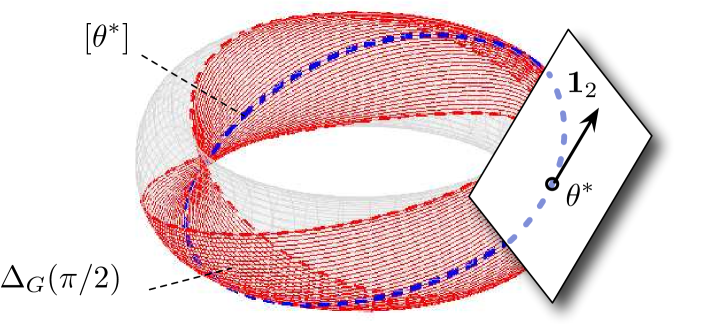
Figure 4: Illustration of the state space $\mathbb{T}^{2}$, the set $\Delta_{G}(\pi/2)$, the synchronization manifold $[\theta^{*}]$ associated to a phase-synchronized angle array $\theta^{*}=$ $(\theta_{1}^{*},\theta_{2}^{*})\in\bar{\Delta}_{G}(0)$, and the tangent space with translation vector $\mathbf{1}_{2}$ at $\theta^{*}$.

III-B A Simple yet Illustrative Example

The following example illustrates the different notions of synchronization introduced above and points out various important geometric subtleties occurring on the compact state space $\mathbb{T}^{2}$. Consider $n=2$ oscillators with $\omega_{2}\geq 0\geq\omega_{1}=-\omega_{2}$. We restrict our attention to angles contained in an open half-circle: for angles $\theta_{1}$, $\theta_{2}$ with $|\theta_{2}-\theta_{1}|<\pi$, the angular difference $\theta_{2}-\theta_{1}$ is the number in ${]\!-\!\pi,\pi[}$ with magnitude equal to the geodesic distance $|\theta_{2}-\theta_{1}|$ and with positive sign if and only if the counter-clockwise path length from $\theta_{1}$ to $\theta_{2}$ on $\mathbb{T}^{1}$ is smaller than the clockwise path length. With this definition the two-dimensional oscillator dynamics $(\dot{\theta}_{1},\dot{\theta}_{2})$ can be reduced to the scalar difference dynamics $\dot{\theta}_{2}-\dot{\theta}_{1}$. After scaling time as $t\mapsto t(\omega_{2}-\omega_{1})$ and introducing $\kappa=2a_{12}/(\omega_{2}-\omega_{1})$ the difference dynamics are

$$\frac{d}{d\,t}\,(\theta_{2}-\theta_{1})=f_{\kappa}(\theta_{2}-\theta_{1}):=1-\kappa\sin(\theta_{2}-\theta_{1})\,.$$ (11)

The scalar dynamics (11) can be analyzed graphically by plotting the vector field $f_{\kappa}(\theta_{2}-\theta_{1})$ over the difference variable $\theta_{2}-\theta_{1}$, as in Figure 5(a). Figure 5(a) displays a saddle-node bifurcation at $\kappa=1$. For $\kappa<1$ no equilibrium of (11) exists, and for $\kappa>1$ an asymptotically stable equilibrium $\theta_{\textup{stable}}=\arcsin(\kappa^{-1})\in{]0,\pi/2[}$ together with a saddle point $\theta_{\textup{saddle}}=\arcsin(\kappa^{-1})\in{]\pi/2,\pi[}$ exists.

For $\theta(0)\in\mbox{Arc}_{n}(|\theta_{\textup{saddle}}|)$ all trajectories converge exponentially to $\theta_{\textup{stable}}$, that is, the oscillators synchronize exponentially. Additionally, the oscillators are phase cohesive if an only if $\theta(0)\in\overline{\mbox{Arc}}_{n}(|\theta_{\textup{saddle}}|)$, where all trajectories remain bounded. For $\theta(0)\not\in\overline{\mbox{Arc}}_{n}(|\theta_{\textup{saddle}}|)$ the difference $\theta_{2}(t)-\theta_{1}(t)$ will increase beyond $\pi$, and by definition will change its sign since the oscillators change orientation. Ultimately, $\theta_{2}(t)-\theta_{1}(t)$ converges to the equilibrium $\theta_{\textup{stable}}$ in the branch where $\theta_{2}-\theta_{1}<0$. In the configuration space $\mathbb{T}^{2}$ this implies that the distance $\left\lvert{\theta_{2}(t)-\theta_{1}(t)}\right\rvert$ increases to its maximum value $\pi$ and shrinks again, that is, the oscillators are not phase cohesive and revolve once around the circle before converging to the equilibrium manifold. Since $\sin(\theta_{\textup{stable}})=\sin(\theta_{\textup{saddle}})=\kappa^{-1}$, strongly coupled oscillators with $\kappa\gg 1$ practically achieve phase synchronization from every initial condition in an open semi-circle. In the critical case, $\kappa=1$, the saddle equilibrium manifold at $\pi/2$ is globally attractive but not stable. An representative trajectory is illustrated in Figure 5(b).

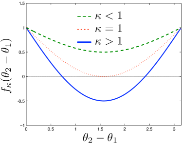
(a) Vector field (11) for $\theta_{2}-\theta_{1}>0$

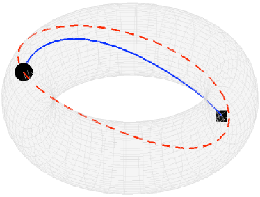
(b) Trajectory $\theta(t)$ for $\kappa=1$

Figure 5: Plot of the vector field (11) for various values of $\kappa$ and a trajectory $\theta(t)\in\mathbb{T}^{2}$ for the critical case $\kappa=1$, where the dashed line is the saddle equilibrium manifold and $\blacksquare$ and $\bf\bullet$ depict $\theta(0)$ and $\lim_{t\to\infty}\theta(t)$. The non-smoothness of the vector field $f(\theta_{2}-\theta_{1})$ at the boundaries $\{0,\pi\}$ is an artifact of the non-smoothness of the geodesic distance on $\mathbb{T}^{2}$

In conclusion, the simple but already rich $2$-dimensional case shows that two oscillators are phase cohesive and synchronize if and only if $\kappa>1$, that is, if and only if the coupling dominates the non-uniformity as $2a_{12}>\omega_{2}-\omega_{1}$. The ratio $1/\kappa$ determines the ultimate phase cohesiveness as well as the set of admissible initial conditions. For $\kappa\gg 1$, practical phase synchronization is achieved for all angles in an open semi-circle. More general coupled oscillator networks display the same phenomenology, but the threshold from incoherence to synchrony is generally unknown.

III-C Synchronization Metrics

The notion of phase cohesiveness can be understood as a performance measure for synchronization and phase synchronization is simply the extreme case of phase cohesiveness with $\lim_{t\to\infty}\theta(t)\in\bar{\Delta}_{G}(0)=\overline{\mbox{Arc}}_{n}(0)$. An alternative performance measure is the magnitude of the so-called order parameter introduced by Kuramoto [5, 6]:

$$re^{\mathrm{i}\psi}=\frac{1}{n}\sum\nolimits_{j=1}^{n}e^{\mathrm{i}\theta_{j}}\,.$$

The order parameter is the centroid of all oscillators represented as points on the unit circle in $\mathbb{C}^{1}$. The magnitude $r$ of the order parameter is a synchronization measure: if all oscillators are phase-synchronized, then $r=1$, and if all oscillators are spaced equally on the unit circle, then $r=0$. The latter case is characterized in Subsection III-E.  For a complete graph, the magnitude $r$ of the order parameter serves as an average performance index for synchronization, and phase cohesiveness can be understood as a worst-case performance index. Extensions of the order parameter tailored to non-complete graphs have been proposed in [52, 19, 56].

For a complete graph and for $\gamma$ sufficiently small, the set $\bar{\Delta}_{G}(\gamma)$ reduces to $\overline{\mbox{Arc}}_{n}(\gamma)$, the arc of length $\gamma$ containing all oscillators. The order parameter is contained within the convex hull of this arc since it is the centroid of all oscillators, see Figure 6. In this case, the magnitude $r$ of the order parameter can be related to the arc length $\gamma$.

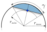
Figure 6: Schematic illustration of an arc of length $\gamma\in{[0,\pi]}$, its convex hull (shaded), and the value ${\color[rgb]{0,0,1}\mathbf{\bullet}}$ of the corresponding order parameter $re^{\mathrm{i}\psi}$ with minimum magnitude $r_{\textup{min}}=\cos(\gamma/2)$ and maximum magnitude $r_{\textup{max}}=1$.

Lemma III.1

(Shortest arc length and order parameter, [74, Lemma 2.1]) Given an angle array $\theta=(\theta_{1},\dots,\theta_{n})\in\mathbb{T}^{n}$ with $n\geq 2$, let $r(\theta)=\frac{1}{n}|\sum_{j=1}^{n}e^{\mathrm{i}\theta_{j}}|$ be the magnitude of the order parameter, and let $\gamma(\theta)$ be the length of the shortest arc containing all angles, that is, $\theta\in\overline{\mbox{Arc}}_{n}(\gamma(\theta))$. The following statements hold:

1. if $\gamma(\theta)\in{[0,\pi]}$, then $r(\theta)\in[\cos(\gamma(\theta)/2),1]$; and

2. if $\theta\in\overline{\mbox{Arc}}_{n}(\pi)$, then $\gamma(\theta)\in[2\arccos(r(\theta)),\pi]$.

III-D Synchronization Conditions

The coupled oscillator dynamics (1) feature (i) the synchronizing coupling described by the graph $G(\mathcal{V},\mathcal{E},A)$ and (ii) the de-synchronizing effect of the non-uniform natural frequencies $\omega$. Loosely speaking, synchronization occurs when the coupling dominates the non-uniformity. Various conditions have been proposed in the synchronization and power systems literature to quantify this trade-off.

The coupling is typically quantified by the algebraic connectivity $\lambda_{2}(L)$ [127, 64, 52, 128, 44, 45] or the weighted nodal degree $\textup{deg}_{i}\triangleq\sum\nolimits_{j=1}^{n}a_{ij}$ [129, 117, 130, 64, 97], and the non-uniformity is quantified by either absolute norms $\|\omega\|_{p}$ or incremental norms $\|B^{T}\omega\|_{p}$, where typically $p\in\{2,\infty\}$. Sometimes, these conditions can be evaluated only numerically since they are state-dependent [127, 129] or arise from a non-trivial linearization process, such as the Master stability function formalism [44, 45, 131]. In general, concise and accurate results are known only for specific topologies such as complete graphs [74], linear chains [108], and bipartite graphs [82] with uniform weights.

For arbitrary coupling topologies only sufficient conditions are known [127, 64, 52, 129] as well as numerical investigations for random networks [132, 89, 128, 98, 99]. Simulation studies indicate that these conditions are conservative estimates on the threshold from incoherence to synchrony. Literally, every review article on synchronization draws attention to the problem of finding sharp synchronization conditions [46, 8, 74, 7, 44, 45, 114].

III-E Phase Balancing and Splay State

In certain applications in neuroscience [11, 12, 13], deep-brain stimulation [26, 27], and vehicle coordination [19, 28, 29, 30, 31], one is not interested in the coherent behavior with synchronized (or nearly synchronized) phases, but rather in the phenomenon of synchronized frequencies and de-sychronized phases.

Whereas the phase-synchronized state is characterized by the order parameter $r$ achieving its maximal (unit) magnitude, we say that a solution $\theta:\,\mathbb{R}_{\geq 0}\to\mathbb{T}^{n}$ to the coupled oscillator model (1) achieves phase balancing if all phases $\theta_{i}(t)$ converge to $\mbox{Bal}_{n}=\{\theta\in\mathbb{T}^{n}:\,r(\theta)=|\frac{1}{n}\sum\nolimits_{j=1}^{n}e^{\mathrm{i}\theta_{j}}|=0\}$ as $t\to\infty$, that is, the oscillators are distributed over the unit circle $\mathbb{S}^{1}$, such that their centroid $re^{\mathrm{i}\psi}$ vanishes. We refer to [28] for a geometric characterization of the balanced state.

One balanced state of particular interest in neuroscience applications [11, 12, 13, 26, 27] is the so-called splay state $\{\theta\in\mathbb{T}^{n}:\,\theta_{i}={i\cdot 2\pi/n+\varphi}\pmod{2\pi}\,,\varphi\in\mathbb{S}^{1}\,,i\in\{1,\dots,n\}\}\subseteq\mbox{Bal}_{n}$ corresponding to phases uniformly distributed around the unit circle $\mathbb{S}^{1}$ with distances $2\pi/n$. Other highly symmetric balanced states consist of multiple clusters of collocated phases, where the clusters themselves are arranged in splay state, see [28, 29].

IV Analysis of Synchronization

In this section we present several analysis approaches to synchronization in the coupled oscillator model (1). We begin with a few basic ideas to provide important intuition as well as the analytic basis for further analysis.

IV-A Some Simple Yet Important Insights

The potential energy $U:\mathbb{T}^{n}\rightarrow\mathbb{R}$ of the elastic spring network in Figure 1 is, up to an additive constant, given by

$$U(\theta)=\sum\nolimits_{\{i,j\}\in\mathcal{E}}a_{ij}\bigl{(}1-\cos(\theta_{i}-\theta_{j})\bigr{)}\,.$$ (12)

By means of the potential energy, the coupled oscillator model (1) can reformulated as the forced gradient system

$$\dot{\theta}_{i}=\omega_{i}-\nabla_{i}U(\theta)\,,\qquad i\in\{1,\dots,n\}\,,$$ (13)

where $\nabla_{i}U(\theta)=\frac{\partial}{\partial\theta_{i}}U(\theta)$ denotes the partial derivative. It can be easily verified that the phase-synchronized state $\theta_{i}=\theta_{j}$ for all $\{i,j\}\in\mathcal{E}$ is a local minimum of the potential energy (12). The gradient formulation (13) clearly emphasizes the competition between the synchronization-enforcing coupling through the potential $U(\theta)$ and the synchronization-inhibiting heterogeneous natural frequencies $\omega_{i}$.

We next note that $\omega$ has to satisfy certain bounds, relative to the weighted nodal degree, in order for a synchronized solution to exist.

Lemma IV.1

(Necessary sync conditions) Consider the coupled oscillator model (1) with graph $G(\mathcal{V},\mathcal{E},A)$, frequencies $\omega\in\mathbf{1}_{n}^{\perp}$, and nodal degree $\textup{deg}_{i}=\sum\nolimits_{j=1}^{n}a_{ij}$ for each oscillator $i\in\{1,\dots,n\}$. If there exists a synchronized solution $\theta\in\bar{\Delta}_{G}(\gamma)$ for some $\gamma\in{[0,\pi/2]}$, then the following conditions hold:

1. Absolute bound: For each node $i\in\{1,\dots,n\}$,

   $$\textup{deg}_{i}\sin(\gamma)\geq|\omega_{i}|\,;$$ (14)

2. Incremental bound: For all distinct $i,j\in\{1,\dots,n\}$,

   $$(\textup{deg}_{i}+\textup{deg}_{j})\sin(\gamma)\geq|\omega_{i}-\omega_{j}|\,.$$ (15)

Proof:

Since $\omega\in\mathbf{1}_{n}^{\perp}$, the synchronization frequency $\omega_{\textup{sync}}$ is zero, and phase and frequency synchronized solutions are equilibrium solutions determined by the equations

$$\omega_{i}=\sum\nolimits_{j=1}^{n}a_{ij}\sin(\theta_{i}-\theta_{j})\,,\qquad i\in\{1,\dots,n\}\,.$$ (16)

Since $\sin(\theta_{i}-\theta_{j})\in{[-\sin(\gamma),+\sin(\gamma)]}$ for $\theta\in\bar{\Delta}_{G}(\gamma)$, the equilibrium equations (16) have no solution if condition (14) is not satisfied. Since $\omega\in\mathbf{1}_{n}^{\perp}$, an incremental bound on $\omega$ seems to be more appropriate than an absolute bound. The subtraction of the $i$th and $j$th equation (16) yields

$$\omega_{i}-\omega_{j}=\sum\nolimits_{k=1}^{n}\left(a_{ik}\sin(\theta_{i}-\theta_{k})-a_{jk}\sin(\theta_{j}-\theta_{k})\right)\,.$$

Again, since the coupling is bounded, the above equation has no solution in $\bar{\Delta}_{G}(\gamma)$ if condition (15) is not satisfied. ∎

The following result is fundamental for various approaches to phase and frequency synchronization. To the best of the authors’ knowledge this result has been first established in [133], and it has been reproved numerous times.

Lemma IV.2

(Stable synchronization in $\Delta_{G}(\pi/2)$) Consider the coupled oscillator model (1) with a connected graph $G(\mathcal{V},\mathcal{E},A)$ and frequencies $\omega\in\mathbf{1}_{n}^{\perp}$. The following statements hold:

1. Jacobian: The Jacobian $J(\theta)$ of the coupled oscillator model (1) evaluated at $\theta\in\mathbb{T}^{n}$ is given by

   $$J(\theta)=-B\operatorname*{\mathrm{diag}}(\{a_{ij}\cos(\theta_{i}-\theta_{j})\}_{\{i,j\}\in\mathcal{E}})B^{T}\,;$$

2. Local stability and uniqueness: If there exists an equilibrium $\theta^{*}\in\Delta_{G}(\pi/2)$, then

   1. $-J(\theta^{*})$ is a Laplacian matrix;

   2. the equilibrium manifold $[\theta^{*}]\in\Delta_{G}(\pi/2)$ is locally exponentially stable; and

   3. this equilibrium manifold is unique in $\bar{\Delta}_{G}(\pi/2)$.

Proof:

Since $\frac{\partial}{\partial\theta_{i}}\bigl{(}\omega_{i}-\sum\nolimits_{j=1}^{n}a_{ij}\sin(\theta_{i}-\theta_{j})\bigr{)}=-\sum\nolimits_{j=1}^{n}a_{ij}\cos(\theta_{i}-\theta_{j})$ and $\frac{\partial}{\partial\theta_{j}}\bigl{(}\omega_{i}-\sum\nolimits_{j=1}^{n}a_{ij}\sin(\theta_{i}-\theta_{j})\bigr{)}=a_{ij}\cos(\theta_{i}-\theta_{j})$, we obtain that the Jacobian is equal to minus the Laplacian matrix of the connected graph $G(\mathcal{V},\mathcal{E},\tilde{A})$ with the (possibly negative) weights $\tilde{a}_{ij}=a_{ij}\cos(\theta_{i}-\theta_{j})$. Equivalently, in compact notation $J(\theta)=-B\operatorname*{\mathrm{diag}}(\{a_{ij}\cos(\theta_{i}-\theta_{j})\}_{\{i,j\}\in\mathcal{E}})B^{T}$. This completes the proof of statement 1).

The Jacobian $J(\theta)$ evaluated for an equilibrium $\theta^{*}\in\Delta_{G}(\pi/2)$ is minus the Laplacian matrix of the graph $G(\mathcal{V},\mathcal{E},\tilde{A})$ with strictly positive weights $\tilde{a}_{ij}=a_{ij}\cos(\theta_{i}^{*}-\theta_{j}^{*})>0$ for every $\{i,j\}\in\mathcal{E}$. Hence, $J(\theta^{*})$ is negative semidefinite with the nullspace $\mathbf{1}_{n}$ arising from the rotational symmetry, see Figure 4. Consequently, the equilibrium point $\theta^{*}\in\Delta_{G}(\pi/2)$ is locally (transversally) exponentially stable, or equivalently, the corresponding equilibrium manifold $[\theta^{*}]\in\Delta_{G}(\pi/2)$ is locally exponentially stable.

The uniqueness statement follows since the right-hand side of the coupled oscillator model (1) is a one-to-one function (modulo rotational symmetry) for $\theta\in\bar{\Delta}_{G}(\pi/2)$, see [134, Corollary 1]. This completes the proof of statement 2). ∎

By Lemma IV.2, any equilibrium in $\Delta_{G}(\pi/2)$ is stable which supports the notion of phase cohesiveness as a performance metric. Since the Jacobian $J(\theta)$ is the negative Hessian of the potential $U(\theta)$ defined in (12), Lemma IV.2 also implies that any equilibrium in $\Delta_{G}(\pi/2)$ is a local minimizer of $U(\theta)$. Of particular interest are so-called $\mathbb{S}^{1}$-synchronizing graphs for which all critical points of (12) are hyperbolic, the phase-synchronized state is the global minimum of $U(\theta)$, and all other critical points are local maxima or saddle points. The class of $\mathbb{S}^{1}$-synchronizing graphs includes, among others, complete graphs and acyclic graphs [100, 101, 102, 103].

These basic insights motivated various characterizations and explorations of the critical points and the curvature of the potential $U(\theta)$ in the literature on synchronization [100, 101, 102, 103, 103, 93, 52, 64, 74, 89, 100] as well as on power systems [133, 135, 116, 61, 136, 134, 129, 127, 137].

IV-B Phase Synchronization

If all natural frequencies are identical, $\omega_{i}\equiv\omega$ for all $i\in\{1,\dots,n\}$, then a transformation of the coupled oscillator model (1) to a rotating frame with frequency $\omega$ leads to

$$\dot{\theta}_{i}=-\sum\nolimits_{j=1}^{n}a_{ij}\sin(\theta_{i}-\theta_{j})\,,\qquad i\in\{1,\dots,n\}\,.$$ (17)

The analysis of the coupled oscillator model (17) is particularly simple and local phase synchronization can be concluded by various analysis methods. A sample of different analysis schemes (by far not complete) includes the contraction property [54, 100, 92, 64, 138], quadratic Lyapunov functions [52, 64], linearization [81, 103], or order parameter and potential function arguments [56, 28, 80].

The following theorem on phase synchronization summarizes a collection of results originally presented in [56, 54, 103, 100, 28, 74], and it can be easily proved given the insights developed in Subsection IV-A.

Theorem IV.3

(Phase synchronization) Consider the coupled oscillator model (1) with a connected graph $G(\mathcal{V},\mathcal{E},A)$ and with frequency $\omega\in\mathbb{R}^{n}$ (not necessarily zero mean). The following statements are equivalent:

1. Stable phase sync: there exists a locally exponentially stable phase-synchronized solution $\theta\in\overline{\mbox{Arc}}_{n}(0)$ (or a synchronization manifold $[\theta]\in\bar{\Delta}_{G}(0)$); and

2. Uniformity: there exists a constant $\omega\in\mathbb{R}$ such that $\omega_{i}=\omega$ for all $i\in\{1,\dots,n\}$.

If the two equivalent cases (i) and (ii) are true, the following statements hold:

1. Global convergence: For all initial angles $\theta(0)\in\mathbb{T}^{n}$ all frequencies $\dot{\theta}_{i}(t)$ converge to $\omega$ and all phases $\theta_{i}(t)-\omega t\pmod{2\pi}$ converge to the critical points $\{\theta\in\mathbb{T}^{n}:\,\nabla U(\theta)=\mathbf{0}_{n}\}$;

2. Semi-global stability: The region of attraction of the phase-synchronized solution $\theta\in\overline{\mbox{Arc}}_{n}(0)$ contains the open semi-circle $\mbox{Arc}_{n}(\pi)$, and each arc $\overline{\mbox{Arc}}_{n}(\gamma)$ is positively invariant for every arc length $\gamma<\pi$;

3. Explicit phase: For initial angles in an open semi-circle $\theta(0)\in\mbox{Arc}_{n}(\pi)$, the asymptotic synchronization phase is given by $\theta(t)\!=\!\sum_{i=1}^{n}\!\theta_{i}(0)/n+\omega t\pmod{2\pi}$;

4. Convergence rate: For every initial angle $\theta(0)\in\overline{\mbox{Arc}}_{n}(\gamma)$ with $\gamma<\pi$, the exponential convergence rate to phase synchronization is no worse than $\lambda_{\textup{ps}}=-\lambda_{2}(L)\operatorname*{sinc}(\gamma)$; and

5. Almost global stability: If the graph $G(\mathcal{V},\mathcal{E},A)$ is $\mathbb{S}^{1}$-synchronizing, the region of attraction of the phase-synchronized solution $\theta\in\overline{\mbox{Arc}}_{n}(0)$ is almost all of $\mathbb{T}^{n}$.

Proof:

Implication (i) $\!\implies\!$ (ii): By assumption, there exist constants $\theta_{\textup{sync}}\in\mathbb{S}^{1}$ and $\omega_{\textup{sync}}\in\mathbb{R}$ such that $\theta_{i}(t)=\theta_{\textup{sync}}+\omega_{\textup{sync}}t\pmod{2\pi}$. In the phase-synchronized case, the dynamics (1) then read as $\omega_{\textup{sync}}=\omega_{i}$ for all $i\in\{1,\dots,n\}$. Hence, a necessary condition for the existence of phase synchronization is that all $\omega_{i}$ are identical.

Implication (ii) $\implies$ (i): Consider the model (1) written in a rotating frame with frequency $\omega$ as in (17). Note that the set of phase-synchronized solutions $\bar{\Delta}_{G}(0)$ is an equilibrium manifold. By Lemma IV.2, we conclude that $\bar{\Delta}_{G}(0)$ is locally exponentially stable. This concludes the proof of (i) $\Leftrightarrow$ (ii).

Statement 1): Note that (17) can be written as the gradient flow $\dot{\theta}=-\nabla U(\theta)$, and the corresponding potential function $U(\theta)$ is non-increasing along trajectories. Since the sublevel sets of $U(\theta)$ are compact and the vector field $\nabla U(\theta)$ is smooth, the invariance principle [139, Theorem 4.4] asserts that every solution converges to set of equilibria of (17).

Statements 2): The coupled oscillator model (17) can be re-written as the consensus-type system

$$\dot{\theta}_{i}=-\sum\nolimits_{j=1}^{n}b_{ij}(\theta)\cdot(\theta_{i}-\theta_{j})\,,\qquad i\in\{1,\dots,n\}\,,$$ (18)

where the weights $b_{ij}(\theta)=a_{ij}\operatorname*{sinc}(\theta_{i}-\theta_{j})$ depend explicitly on the system state. Notice that for $\theta\in\overline{\mbox{Arc}}_{n}(\gamma)$ and $\gamma<\pi$ the weights $b_{ij}(\theta)$ are upper and lower bounded as $b_{ij}(\theta)\in{[a_{ij}\operatorname*{sinc}(\gamma),a_{ij}]}$ Assume that the initial angles $\theta_{i}(0)$ belong to the set $\overline{\mbox{Arc}}_{n}(\gamma)$, that is, they are all contained in an arc of length $\gamma\in{[0,\pi[}$. In this case, a natural Lyapunov function to establish phase synchronization can be obtained from the contraction property, which aims at showing that the convex hull containing all oscillators is decreasing, see [140, 54, 100, 92, 64] and the review [138, Section 2].

Recall the geodesic distance between two angles on $\mathbb{S}^{1}$ and define the continuous function $V:\mathbb{T}^{n}\rightarrow[0,\pi]$ by

$$V(\psi)=\max\{|\psi_{i}-\psi_{j}|\;|\;i,j\in\{1,\dots,n\}\}.$$ (19)

Notice that, if all angles are contained in an arc at time $t$, then the arc length $V(\theta(t))=\max_{i,j\in\{1,\dots,n\}}|\theta_{i}(t)-\theta_{j}(t)|$ is a Lyapunov function candidate for phase synchronization. Indeed, it can be shown that $V(\theta(t))$ decreases along trajectories of (18) for $\theta(0)\in\overline{\mbox{Arc}}_{n}(\gamma)$ and for all $\gamma<\pi$. The analysis is complicated by the following fact: the function $V(\theta(t))$ is continuous but not necessarily differentiable when the maximum geodesic distance (that is, the right-hand side of (19)), is attained by more than one pair of oscillators. We omit the explicit calculations here and refer to [54, 92, 83, 64, 74] for a detailed analysis.

Statement 3): By statement 2), the set $\mbox{Arc}_{n}(\pi)$ is positively invariant, and for $\theta(0)\in\mbox{Arc}_{n}(\pi)$ the average $\sum_{i=1}^{n}\theta_{i}(t)/n$ is well defined for $t\geq 0$. A summation over all equations of the model (17) yields $\sum\nolimits_{i=1}^{n}\dot{\theta}_{i}(t)=0$, or equivalently, $\sum_{i=1}^{n}\theta_{i}(t)$ is constant for all $t\geq 0$. In particular, for $t=0$ we have that $\sum_{i=1}^{n}\theta_{i}(t)=\sum_{i=1}^{n}\theta_{i}(0)$ and for a phase-synchronized solution we have that $\sum_{i=1}^{n}\theta_{\textup{sync}}=\sum_{i=1}^{n}\theta_{i}(0)$. Hence, the explicit synchronization phase is given by $\sum_{i=1}^{n}\theta_{i}(0)/n$. In the original coordinates (non-rotating frame) the synchronization phase is given by $\sum_{i=1}^{n}\theta_{i}(0)/n+\omega t\pmod{2\pi}$.

Statement 4): Given the invariance of the set $\overline{\mbox{Arc}}_{n}(\gamma)$ for any $\gamma<\pi$, the system (18) can be analyzed as a linear time-varying consensus system with initial condition $\theta(0)\in\overline{\mbox{Arc}}_{n}(\gamma)$, and bounded time-varying weights $b_{ij}(\theta(t))\in{[a_{ij}\operatorname*{sinc}(\gamma),a_{ij}]}$ for all $t\geq 0$. The worst-case convergence rate $\lambda_{\textup{ps}}$ can then be obtained by a standard symmetric consensus analysis, see [53, 52, 64, 74]. For instance, it can be shown that the deviation of the angles $\theta(t)$ from their average, $\|\theta(t)-(\sum_{i=1}^{n}\theta(t)/n)\mathbf{1}_{n}\|_{2}^{2}$ (the disagreement function) decays exponentially with rate $\lambda_{\textup{ps}}$.

Statement 5): By statement 1), all solutions of system (17) converge to the set of equilibria, which equals the set of critical points of the potential $U(\theta)$. By the definition of $\mathbb{S}^{1}$-synchronizing graphs, the phase-synchronized equilibrium manifold $\overline{\mbox{Arc}}_{n}(0)$ is the only stable equilibrium set, and all others are unstable. Hence, for all initial condition $\theta(0)\in\mathbb{T}^{n}$, which are not on the stable manifolds of unstable equilibria, the corresponding solution $\theta(t)$ will reach the phase-synchronized equilibrium manifold $\overline{\mbox{Arc}}_{n}(0)$. ∎

Remark 2

(Control-theoretic perspective on synchronization) As established in Theorem IV.3, the set of phase-synchronized solutions $\overline{\mbox{Arc}}_{n}(0)$ of the coupled oscillator model (1) is locally stable provided that all natural frequencies are identical. For non-uniform (but sufficiently identical) natural frequencies, phase synchronization is not possible but a certain degree of phase cohesiveness can still be achieved. Hence, the coupled oscillator model (1) can be regarded as an exponentially stable system subject to the disturbance $\omega\in\mathbf{1}_{n}^{\perp}$, and classic control-theoretic concepts such as input-to-state stability, practical stability, and ultimate boundedness [139] or their incremental versions [141] can be used to study synchronization. In control-theoretic terminology, synchronization and phase cohesiveness can then also be described as “practical phase synchronization”. Compared to prototypical nonlinear control examples, various additional challenges arise in the analysis of the coupled oscillator model (1) due to the bounded and non-monotone sinusoidal coupling and the compact state space $\mathbb{T}^{n}$ containing numerous equilibria; see the analysis approaches in Section IV and [95, 74, 64]. $\square$

IV-C Phase Balancing

In general, only few results are known about the phase balancing problem. This asymmetry is partially caused by the fact that phase synchrony is required in more applications than phase balancing. Moreover, the phase-synchronized set $\overline{\mbox{Arc}}_{n}(0)$ admits a very simple geometric characterization, whereas the phase-balanced set $\mbox{Bal}_{n}$ has a complicated structure consisting of numerous disjoint subsets. The number of these subsets grows with the number of nodes $n$ in a combinatorial fashion.

Consider the coupled oscillator model (17) with identical natural frequencies. By inverting the direction of time, we get

$$\dot{\theta}_{i}=\sum\nolimits_{j=1}^{n}a_{ij}\sin(\theta_{i}-\theta_{j})\,,\qquad i\in\{1,\dots,n\}\,.$$ (20)

In the following, we say that the interaction graph $G(\mathcal{V},\mathcal{E},A)$ is circulant if the adjacency matrix $A=A^{T}$ is a circulant matrix. Circulant graphs are highly symmetric graphs including complete graphs, bipartite graphs, and ring graphs. For circulant and uniformly weighted graphs, the coupled oscillator model (20) achieves phase balancing. The following theorem summarizes different results, which were originally presented in [28, 29].

Theorem IV.4

(Phase balancing) Consider the coupled oscillator model (20) with a connected, uniformly weighted, and circulant graph $G(\mathcal{V},\mathcal{E},A)$. The following statements hold:

1. Local phase balancing: The phase-balanced set $\mbox{Bal}_{n}$ is locally asymptotically stable; and

2. Almost global stability: If the graph $G(\mathcal{V},\mathcal{E},A)$ is complete, then the region of attraction of the stable phase-balanced set $\mbox{Bal}_{n}$ is almost all of $\mathbb{T}^{n}$.

The proof of Theorem IV.4 follows a similar reasoning as the proof of Theorem IV.3: convergence is established by potential function arguments and local (in)stability of equilibria by Jacobian arguments. We omit the proof here and refer to [28, Theorem 1] and [29, Theorem 2] for details.

For general connected graphs, the conclusions of Theorem IV.4 are not true. As a remedy to achieve locally stable and globally attractive phase balancing, higher order models need to be considered, see the models proposed in [56, 29].

IV-D Synchronization in Complete Networks

For a complete coupling graph with uniform weights $a_{ij}=K/n$, where $K>0$ is the coupling gain, the coupled oscillator model (1) reduces to the celebrated Kuramoto model

$$\dot{\theta}_{i}=\omega_{i}-\frac{K}{n}\sum\nolimits_{j=1}^{n}\sin(\theta_{i}-\theta_{j})\,,\qquad i\in\{1,\dots,n\}\,.$$ (21)

By means of the order parameter $re^{\mathrm{i}\psi}=\frac{1}{n}\sum_{j=1}^{n}e^{\mathrm{i}\theta_{j}}$, the Kuramoto model (21) can be rewritten in the insightful form

$$\dot{\theta}_{i}=\omega_{i}-Kr\sin(\theta_{i}-\psi)\,,\quad i\in\{1,\dots,n\}\,.$$ (22)

Equation (22) gives the intuition that the oscillators synchronize by coupling to a mean field represented by the order parameter $re^{\mathrm{i}\psi}$. Intuitively, for small coupling strength $K$ each oscillator rotates with its natural frequency $\omega_{i}$, whereas for large coupling strength $K$ all angles $\theta_{i}(t)$ will be entrained by the mean field $re^{\mathrm{i}\psi}$ and the oscillators synchronize. The threshold from incoherence to synchronization occurs for some critical coupling $K_{\textup{critical}}$. This phase transition has been the source of numerous investigations starting with Kuramoto’s analysis [5, 6]. Various necessary, sufficient, implicit, and explicit estimates of the critical coupling strength $K_{\textup{critical}}$ for both the on-set as well as the ultimate stage of synchronization have been proposed [5, 74, 7, 8, 28, 64, 6, 87, 110, 104, 53, 52, 105, 106, 75, 86, 84, 85, 107, 103, 82, 100, 97, 95, 83, 96], and we refer to [74] for a comprehensive overview.

The mean field approach to the equations (22) can be made mathematically rigorous by a time-scale separation [96] or in the continuum limit as the number of oscillators tends to infinity and the natural frequencies $\omega$ are sampled from a distribution function $g:\mathbb{R}\to\mathbb{R}_{\geq 0}$. In the continuum limit and for a symmetric, continuous, and unimodal distribution $g(\omega)$, Kuramoto himself showed in an insightful and ingenuous analysis [5, 6] that the incoherent state (a uniform distribution of the oscillators on the unit circle $\mathbb{S}^{1}$) supercritically bifurcates for the critical coupling strength

$$K_{\textup{critical}}=\frac{2}{\pi g(0)}\,.$$ (23)

In [87, 104, 8], it was found that the bipolar (bimodal double-delta) distribution (respectively the uniform distribution) yield the largest (respectively smallest) threshold $K_{\textup{critical}}$ over all distributions $g(\omega)$ with bounded support. We refer [7, 8] for further references and to [111, 109, 88, 110] for recent contributions on the continuum limit model.

In the finite-dimensional case, the necessary synchronization condition (15) gives a lower bound for $K_{\textup{critical}}$ as

$$K\geq\frac{n}{2(n-1)}\cdot(\omega_{\textup{max}}-\omega_{\textup{min}})\,.$$ (24)

Three recent articles [86, 84, 85] independently derived a set of implicit consistency equations for the exact critical coupling strength $K_{\textup{critical}}$ for which synchronized solutions exist. Verwoerd and Mason provided the following implicit formulae to compute $K_{\textup{critical}}$ [86, Theorem 3]:

$$\begin{split}&K_{\textup{critical}}=nu^{*}/\sum\nolimits_{i=1}^{n}\sqrt{1-(\Omega_{i}/u^{*})^{2}}\,,\\ &\!2\sum\nolimits_{i=1}^{n}\!\sqrt{1-(\Omega_{i}/u^{*})^{2}}=\sum\nolimits_{i=1}^{n}\!1/\sqrt{1-(\Omega_{i}/u^{*})^{2}},\end{split}$$ (25)

where $\Omega_{i}=\omega_{i}-\omega_{\textup{sync}}$ and $u^{*}\in[\left\lVert{\Omega}\right\rVert_{\infty},2\left\lVert{\Omega}\right\rVert_{\infty}]$. The implicit formulae (25) can also be extended to bipartite graphs [82]. A local stability analysis is carried out in [84, 85].

From the point of analyzing or designing a sufficiently strong coupling, the exact formulae (25) have three drawbacks. First, they are implicit and thus not suited for performance or robustness estimates in case of additional coupling strength for a given $K>K_{\textup{critical}}$. Second, the corresponding region of attraction of a synchronized solution is unknown. Third and finally, the particular natural frequencies $\omega_{i}$ are typically time-varying, uncertain, or even unknown in the applications listed in Section I. In this case, the exact value of $K_{\textup{critical}}$ needs to be estimated in continuous time, or a conservatively strong coupling $K\!\gg\!K_{\textup{critical}}$ has to be chosen.

The following theorem states an explicit bound on the critical coupling strength together with performance estimates, convergence rates, and a guaranteed semi-global region of attraction for synchronization. This bound is tight and thus necessary and sufficient when considering arbitrary distributions of the natural frequencies with compact support. The result has been originally presented in [74, Theorem 4.1].

Theorem IV.5

(Synchronization in the Kuramoto model) Consider the Kuramoto model (21) with natural frequencies $\omega=(\omega_{1},\dots,\omega_{n})$ and coupling strength $K$. The following three statements are equivalent:

1. the coupling strength $K$ is larger than the maximum non-uniformity among the natural frequencies, that is,

   $$K>K_{\textup{critical}}\triangleq\omega_{\textup{max}}-\omega_{\textup{min}}\;;$$ (26)

2. there exists an arc length $\gamma_{\textup{max}}\in{]\pi/2,\pi]}$ such that the Kuramoto model (21) synchronizes exponentially for all possible distributions of the natural frequencies $\omega_{i}$ supported on the compact interval $[\omega_{\textup{min}},\omega_{\textup{max}}]$ and for all initial phases $\theta(0)\in\mbox{Arc}_{n}(\gamma_{\textup{max}})$; and

3. there exists an arc length $\gamma_{\textup{min}}\in{[0,\pi/2[}$ such that the Kuramoto model (21) has a locally exponentially stable synchronization manifold in $\overline{\mbox{Arc}}_{n}(\gamma_{\textup{min}})$ for all possible distributions of the natural frequencies $\omega_{i}$ supported on the compact interval $[\omega_{\textup{min}},\omega_{\textup{max}}]$.

If the three equivalent conditions (i), (ii), and (iii) hold, then the ratio $K_{\textup{critical}}/K$ and the arc lengths $\gamma_{\textup{min}}\in{[0,\pi/2[}$ and $\gamma_{\textup{max}}\in{]\pi/2,\pi]}$ are related uniquely via $\sin(\gamma_{\textup{min}})=\sin(\gamma_{\textup{max}})={K_{\textup{critical}}}/K$, and the following statements hold:

1. phase cohesiveness: the set $\overline{\mbox{Arc}}_{n}(\gamma)\subseteq\bar{\Delta}_{G}(\gamma)$ is positively invariant for every $\gamma\in[\gamma_{\textup{min}},\gamma_{\textup{max}}]$, and each trajectory starting in $\mbox{Arc}_{n}(\gamma_{\textup{max}})$ approaches asymptotically $\overline{\mbox{Arc}}_{n}(\gamma_{\textup{min}})$;

2. frequency synchronization: the asymptotic synchronization frequency is the average frequency $\omega_{\textup{sync}}=\frac{1}{n}\sum_{i=1}^{n}\omega_{i}$, and, given phase cohesiveness in $\overline{\mbox{Arc}}_{n}(\gamma)$ for some fixed $\gamma<\pi/2$, the exponential synchronization rate is no worse than $\lambda_{\textup{K}}=-K\cos(\gamma)$; and

3. order parameter: the asymptotic value of the magnitude of the order parameter, denoted by $r_{\infty}\triangleq\lim_{t\to\infty}\frac{1}{n}|\sum_{j=1}^{n}e^{\mathrm{i}\theta_{j}(t)}|$, is bounded as

   $$1\geq r_{\infty}\geq\cos\!\left(\frac{\gamma_{\textup{min}}}{2}\right)=\sqrt{\frac{1+\sqrt{1-(K_{\textup{critical}}/K)^{2}}}{2}}\,.$$

Proof:

In the following, we sketch the proof of Theorem IV.5 and refer to [74, Theorem 4.1] for further details.

Implication (i) $\implies$ (ii): In a first step, it is shown that the phase cohesive set $\overline{\mbox{Arc}}_{n}(\gamma)$ is positively invariant for every $\gamma\in[\gamma_{\textup{min}},\gamma_{\textup{max}}]$. By assumption, the angles $\theta_{i}(t)$ belong to the set $\overline{\mbox{Arc}}_{n}(\gamma)$ at time $t=0$, that is, they are all contained in an arc of length $\gamma$. We aim to show that all angles remain in $\overline{\mbox{Arc}}_{n}(\gamma)$ for all subsequent times $t>0$ by means of the contraction Lyapunov function (19). Note that $\overline{\mbox{Arc}}_{n}(\gamma)$ is positively invariant if and only if $V(\theta(t))$ does not increase at any time $t$ such that $V(\theta(t))=\gamma$. The upper Dini derivative of $V(\theta(t))$ along trajectories of (21) is given by

$$D^{+}V(\theta(t))=\lim_{h\downarrow 0}\sup\frac{V(\theta(t+h))-V(\theta(t))}{h}\,.$$

Written out in components and after trigonometric simplifications [74], we obtain that the derivative is bounded as

$$D^{+}V(\theta(t))\leq\omega_{\textup{max}}-\omega_{\textup{min}}-K\sin(\gamma)\,.$$

It follows that the length of the arc formed by the angles is non-increasing in $\overline{\mbox{Arc}}_{n}(\gamma)$ if and only if

$$K\sin(\gamma)\geq K_{\textup{critical}}\,,$$ (27)

where $K_{\textup{critical}}$ is as stated in equation (26). For $\gamma\in{[0,\pi]}$ the left-hand side of (27) is a concave function of $\gamma$ that achieves its maximum at $\gamma^{*}=\pi/2$. Therefore, there exists an open set of arc lengths $\gamma\in{[0,\pi]}$ satisfying equation (27) if and only if equation (27) is true with the strict equality sign at $\gamma^{*}=\pi/2$, which corresponds to condition (26). Additionally, if these two equivalent statements are true, then there exists a unique $\gamma_{\textup{min}}\in{[0,\pi/2[}$ and a $\gamma_{\textup{max}}\in{]\pi/2,\pi]}$ that satisfy equation (27) with the equality sign, namely $\sin(\gamma_{\textup{min}})=\sin(\gamma_{\textup{max}})={K_{\textup{critical}}}/K$. For every $\gamma\in{[\gamma_{\textup{min}},\gamma_{\textup{max}}]}$ it follows that the arc-length $V(\theta(t))$ is non-increasing, and it is strictly decreasing for $\gamma\in{]\gamma_{\textup{min}},\gamma_{\textup{max}}[}$. Among other things, this shows that statement (i) implies statement 1). By means of Lemma III.1, statement 3) then follows from statement 1).

The frequency dynamics of the Kuramoto model (21) can be obtained by differentiating the Kuramoto model (21) as

$$\frac{d}{d\,t}\,\dot{\theta_{i}}=\sum\nolimits_{j=1}^{n}\tilde{a}_{ij}(t)\,(\dot{\theta}_{j}-\dot{\theta}_{i})\,,$$ (28)

where $\tilde{a}_{ij}(t)=(K/n)\cos(\theta_{i}(t)-\theta_{j}(t))$. For $K>K_{\textup{critical}}$, we just proved that for every $\theta(0)\in\mbox{Arc}_{n}(\gamma_{\textup{max}})$ and for all $\gamma\in{]\gamma_{\textup{min}},\gamma_{\textup{max}}[}$ there exists a finite time $T\geq 0$ such that $\theta(t)\in\overline{\mbox{Arc}}_{n}(\gamma)$ for all $t\geq T$. Consequently, the terms $\tilde{a}_{ij}(t)$ are strictly positive for all $t\geq T$. Notice also that system (28) evolves on the tangent space of $\mathbb{T}^{n}$, that is, the Euclidean space $\mathbb{R}^{n}$. Now fix $\gamma\in{]\gamma_{\textup{min}},\pi/2[}$ and let $T\geq 0$ such that $\tilde{a}_{ij}(t)>0$ for all $t\geq T$. In this case, the frequency dynamics (28) can be analyzed as linear time-varying consensus system. Consider the disagreement vector $x=\dot{\theta}-\omega_{\textup{sync}}\mathbf{1}_{n}$ as an error coordinate. By standard consensus arguments [48, 49, 50], it can be shown that the disagreement vector satisfies $\|x(t)\|\!\leq\!\|x(0)\|e^{-\lambda_{\textup{K}}t}$ for all $t\geq T$. This proves statement 2) and the implication (i) $\implies$ (ii).

Implication (ii) $\implies$ (i): To show that condition (26) is also necessary for synchronization, it suffices to construct a counter example for which $K\leq K_{\textup{critical}}$ and the oscillators do not achieve exponential synchronization even though all $\omega_{i}\in{[\omega_{\textup{min}},\omega_{\textup{max}}]}$ and $\theta(0)\in\mbox{Arc}_{n}(\gamma)$ for every $\gamma\in{]\pi/2,\pi]}$. A basic instability mechanism under which synchronization breaks down is caused by a bipolar distribution of the natural frequencies. Let the index set $\{1,\dots,n\}$ be partitioned by the two non-empty sets $\mathcal{I}_{1}$ and $\mathcal{I}_{2}$. Let $\omega_{i}=\omega_{\textup{min}}$ for $i\in\mathcal{I}_{1}$ and $\omega_{i}=\omega_{\textup{max}}$ for $i\in\mathcal{I}_{2}$, and assume that at some time $t\geq 0$ it holds that $\theta_{i}(t)\!=\!-\gamma/2$ for $i\in\mathcal{I}_{1}$ and $\theta_{i}(t)\!=\!+\gamma/2$ for $i\in\mathcal{I}_{2}$ and for some $\gamma\in{[0,\pi[}$. By construction, at time $t$ all oscillators are contained in an arc of length $\gamma\in{[0,\pi[}$. Assume now that $K\!<\!K_{\textup{critical}}$ and the oscillators synchronize. It can be shown [74] that the evolution of the arc length $V(\theta(t))$ satisfies the equality

$$D^{+}V(\theta(t))=\omega_{\textup{max}}-\omega_{\textup{min}}-K\sin(\gamma)\,.$$ (29)

Clearly, for $K<K_{\textup{critical}}$ the arc length $V(\theta(t))=\gamma$ is increasing for any arbitrary $\gamma\in{[0,\pi]}$. Thus, the phases are not bounded in $\overline{\mbox{Arc}}_{n}(\gamma)$. This contradicts the assumption that the oscillators synchronize for $K<K_{\textup{critical}}$ from every initial condition $\theta(0)\in\overline{\mbox{Arc}}_{n}(\gamma)$. For $K=K_{\textup{critical}}$, we know from [84, 85] that phase-locked equilibria have a zero eigenvalue with a two-dimensional Jacobian block, and thus synchronization cannot occur. This instability via a two-dimensional Jordan block is also visible in (29) since $D^{+}V(\theta(t))$ is increasing for $\theta(t)\in\overline{\mbox{Arc}}_{n}(\gamma)$, $\gamma\in{]\pi/2,\pi]}$ until all oscillators change orientation, just as in the example in Subsection III-B. This proves the implication (ii) $\implies$ (i).

Equivalence (i),(ii) $\Leftrightarrow$ (iii): The proof relies on Jacobian arguments and will be omitted here, see [74] for details. ∎

Theorem IV.5 places a hard bound on the critical coupling strength $K_{\textup{critical}}$ for all distributions of $\omega_{i}$ supported on the compact interval $[\omega_{\textup{min}},\omega_{\textup{max}}]$. For a particular distribution $g(\omega)$ supported on $[\omega_{\textup{min}},\omega_{\textup{max}}]$ the bound (26) is only sufficient and possibly a factor 2 larger than the necessary bound (24). The exact critical coupling lies somewhere in between and can be obtained from the implicit equations (25).

Since the bound (26) on $K_{\textup{critical}}$ is exact [74] for the worst-case bipolar distribution $\omega_{i}\in\{\omega_{\textup{min}},\omega_{\textup{max}}\}$, Figure 7 reports numerical findings for the other extreme case [87] of a uniform distribution $g(\omega)=1/2$ supported for $\omega_{i}\in[-1,1]$.

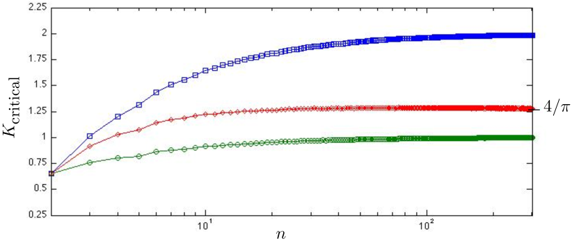
Figure 7: Statistical analysis of the necessary and explicit bound (24) ($\color[rgb]{0,1,0}\lozenge$), the exact and implicit bound (25) ($\color[rgb]{1,0,0}{\circ}$), and the sufficient, tight, and explicit bound (26) ($\color[rgb]{0,0,1}{\square}$) for $n\in[2,300]$ oscillators in a semi-log plot, where the coupling gains for each $n$ are averaged over 1000 simulations.

All three displayed bounds are identical for $n=2$ oscillators. As $n$ increases, the sufficient bound (26) converges to the width $\omega_{\textup{max}}-\omega_{\textup{min}}=2$ of the support of $g(\omega)$, and the necessary bound (24) accordingly to half of the width. The exact bound (25) converges to $4(\omega_{\textup{max}}-\omega_{\textup{min}})/(2\pi)\!=\!4/\pi$ in agreement with condition (23) predicted for the continuum limit.

Finally, let us mention that Theorem IV.5 can be extended to discontinuously switching and slowly time-varying natural frequencies [74]. For a particular sampling distribution $g(\omega)$, the critical quantity in condition (26), the support $\omega_{\textup{max}}-\omega_{\textup{min}}$, can be estimated by extreme value statistics, see [89].

IV-E Synchronization in Sparse Networks

As summarized in Subsection III-D, the quest for sharp and concise synchronization for non-complete coupling graph $G(\mathcal{V},\mathcal{E},A)$ is an important and outstanding problem emphasized in every review article on coupled oscillator networks [46, 8, 74, 7, 44, 45]. The approaches known for phase synchronization in arbitrary graphs or the contraction approach to frequency synchronization (used in the proof of Theorem IV.5) do not generally extend to arbitrary natural frequencies $\omega\in\mathbf{1}_{n}^{\perp}$ and connected coupling graphs $G(\mathcal{V},\mathcal{E},A)$, or do so only under extremely conservative conditions.

One Lyapunov function advocated for classic Kuramoto oscillators (21) is the function $W:\,\mbox{Arc}_{n}(\pi)\to\mathbb{R}$ defined for angles $\theta$ in an open semi-circle and given by [53, 52]

$$W(\theta)=\frac{1}{4}\sum\nolimits_{i,j=1}^{n}|\theta_{i}-\theta_{j}|^{2}=\frac{1}{2}\left\|B_{c}^{T}\theta\right\|_{2}^{2}\,,$$ (30)

where $B_{c}\in\mathbb{R}^{n\times(n(n-1)/2)}$ is an incidence matrix of the complete graph. As shown in [64, Theorem 4.4], the Lyapunov function (30) generalizes also to the coupled oscillator model (1). Indeed, an even more general model is considered in [64], and a Lyapunov analysis yields the following result.

Theorem IV.6

(Frequency synchronization I) Consider the coupled oscillator model (1) with a connected graph $G(\mathcal{V},\mathcal{E},A)$ and $\omega\in\mathbf{1}_{n}^{\perp}$. Assume that the algebraic connectivity is larger than a critical value, that is,

$$\lambda_{2}(L)>\lambda_{\textup{critical}}\triangleq\left\lVert{B_{c}^{T}\omega}\right\rVert_{2}\,,$$ (31)

where $B_{c}\in\mathbb{R}^{n\times n(n-1)/2}$ is the incidence matrix of the complete graph. Accordingly, define $\gamma_{\textup{max}}\in{]\pi/2,\pi]}$ and $\gamma_{\textup{min}}\in{[0,\pi/2[}$ as unique solutions to $(\pi/2)\cdot\operatorname*{sinc}(\gamma_{\textup{max}})\!=\!\sin(\gamma_{\textup{min}})\!=\!\lambda_{\textup{critical}}/\lambda_{2}(L)$. The following statements hold:

1. phase cohesiveness: the set $\bigl{\{}\theta\in\mbox{Arc}_{n}(\pi):\,\|B_{c}^{T}\theta\|_{2}\leq\gamma\bigr{\}}\subseteq\bar{\Delta}_{G}(\gamma)$ is positively invariant for every $\gamma\in[\gamma_{\textup{min}},\gamma_{\textup{max}}]$, and each trajectory starting in the set $\bigl{\{}\theta\in\mbox{Arc}_{n}(\pi):\,\left\lVert{B_{c}^{T}\theta}\right\rVert_{2}<\gamma_{\textup{max}}\bigr{\}}$ asymptotically reaches the set $\bigl{\{}\theta\in\mbox{Arc}_{n}(\pi):\,\|B_{c}^{T}\theta\|_{2}\leq\gamma_{\textup{min}}\bigr{\}}$; and

2. frequency synchronization: for every $\theta(0)\in\mbox{Arc}_{n}(\pi)$ with $\left\lVert{B_{c}^{T}\theta(0)}\right\rVert_{2}<\gamma_{\textup{max}}$ the frequencies $\dot{\theta}_{i}(t)$ synchronize exponentially to the average frequency $\omega_{\textup{sync}}=\frac{1}{n}\sum_{i=1}^{n}\omega_{i}$, and, given phase cohesiveness in $\bar{\Delta}_{G}(\gamma)$ for some fixed $\gamma<\pi/2$, the exponential synchronization rate is no worse than $\lambda_{\textup{fe}}=-\lambda_{2}(L)\cos(\gamma)$.

The proof of Theorem IV.6 follows a similar ultimate-boundedness strategy as the proof of Theorem IV.5 by using the Lyapunov function (30). It can be found in Appendix -B.

For classic Kuramoto oscillators (21), condition (31) reduces to $K>\left\lVert{B_{c}^{T}\omega}\right\rVert_{2}$. Clearly, the condition $K\!>\!\left\lVert{B_{c}^{T}\omega}\right\rVert_{2}$ is more conservative than the bound (26) which reads as $K>\|B_{c}^{T}\omega\|_{\infty}=\omega_{\textup{max}}-\omega_{\textup{min}}$. One reason for this conservatism is that the analysis leading to condition (31) requires all phase distances $|\theta_{i}-\theta_{j}|$ to be bounded, whereas according to Lemma IV.2 only pairwise  phase distances $|\theta_{i}-\theta_{j}|$, $\{i,j\}\in\mathcal{E}$, need to be bounded for stable synchronization. The following result exploits these weaker assumptions and states a sharper (but only local) synchronization condition.

Theorem IV.7

(Frequency synchronization II) Consider the coupled oscillator model (1) with a connected graph $G(\mathcal{V},\mathcal{E},A)$ and $\omega\in\mathbf{1}_{n}^{\perp}$. There exists a locally exponentially stable equilibrium manifold $[\theta]\in\Delta_{G}(\pi/2)$ if

$$\lambda_{2}(L)>\left\|B^{T}\omega\right\|_{2}\,.$$ (32)

Moreover, if condition (32) holds, then $[\theta]$ is phase cohesive in $\{\theta\in\mathbb{T}^{n}:\,\|B^{T}\theta\|_{2}\leq\gamma_{\textup{min}}\}\subseteq\bar{\Delta}_{G}(\gamma_{\textup{min}})$, where $\gamma_{\textup{min}}\in{[0,\pi/2[}$ satisfies $\sin(\gamma_{\textup{min}})=\|B^{T}\omega\|_{2}/\lambda_{2}(L)$.

The strategy to prove Theorem IV.7 is inspired by the ingenuous analysis in [52, Section IIV.B]. It relies on the insight gained from Lemma IV.2 that any synchronization manifold $[\theta]\in\Delta_{G}(\pi/2)$ is locally stable, and it formulates the existence of such a synchronization manifold as a fixed point problem. Here, we follow the basic proof strategy in [52], but we provide a more accurate result together with a self-contained proof which is reported in Appendix -C.

V Conclusions and Open Research Directions

In this paper we introduced the reader to the coupled oscillator model (1), we reviewed several applications, we discussed different synchronization notions, and we presented different analysis approaches to phase synchronization, phase balancing, and frequency synchronization.

Despite the vast literature, the countless applications, and the numerous theoretic results on the synchronization properties of model (1), many interesting and important problems are still open. In the following, we summarize limitations of the existing analysis approaches and present a few worthwhile directions for future research.

First, in many applications the coupling between the oscillators is not purely sinusoidal. For instance, phase delays in neuroscience [13], time delays in sensor networks [37], or transfer conductances in power networks [63] lead to a “shifted coupling” of the form $\sin(\theta_{i}-\theta_{j}-\varphi_{ij})$, where $\varphi_{ij}\in{[-\pi/2,\pi/2]}$. In this case and also for other “skewed” or “symmetry-breaking” coupling functions, many of the presented analysis schemes either fail or lead to overly conservative results. Another interesting class of oscillator networks are systems of pulse-coupled oscillators featuring hybrid dynamics: impulsive coupling at discrete time instants and uncoupled continuous dynamics otherwise. This class of oscillator networks displays a very interesting phenomenology. For instance, the behavior of identical oscillators coupled in a complete graph strongly depends on the curvature of the uncoupled dynamics [142]. Most of the results known for continuously-coupled oscillators still need to be extended to pulse-coupled oscillators with hybrid dynamics.

Second, in many applications [34, 12, 24, 63, 67] the coupled oscillator dynamics are not given by a simple first-order phase model of the form (1). Rather, the dynamics are of higher order, or sometimes there is no readily available phase variable to describe the limit cycle attracting the coupled dynamics. The analysis of oscillator networks with more general oscillator dynamics is largely unexplored. Whereas advances have been made for the simple case of phase synchronization of linear or passive oscillator networks, the case of frequency synchronization of non-identical oscillators with higher-order dynamics is not well-studied.

Third, despite the vast scientific interest the quest for sharp, concise, and closed-form synchronization conditions for arbitrary complex graphs has been so far in vain [46, 8, 74, 7, 44, 45]. As suggested by Lemma IV.1, Lemma IV.2, Theorem IV.5, and the proof of Theorem IV.7, the proper metric for the synchronization problem is the incremental $\infty$-norm $\|B^{T}\theta\|_{\infty}=\max_{\{i,j\}\in\mathcal{E}}|\theta_{i}-\theta_{j}|$. In the authors’ opinion, a Banach space analysis of the coupled oscillator model (1) with the incremental $\infty$-norm will most likely deliver the sharpest possible conditions. However, such an analysis is very challenging for arbitrary natural frequencies $\omega\in\mathbf{1}_{n}^{\perp}$ and connected and weighted coupling graphs $G(\mathcal{V},\mathcal{E},A)$. Recent work [114] by the authors puts forth a novel algebraic condition for synchronization with a rigorous analysis for specific classes of graphs and with (only) a statistical validation for generic weighted graphs.

Fourth and finally, a few interesting and open theoretical challenges include the following. First, most of the presented analysis approaches and conditions do not extend to time-varying or directed coupling graphs $G(\mathcal{V},\mathcal{E},A)$, and alternative methods need to be developed. Second, most known estimates on the region of attraction of a synchronized solution are conservative. The semi-circle estimates given in Theorem IV.3 and Theorem IV.5 rely on convexity of $\mbox{Arc}_{n}(\pi)$ and are overly conservative. We refer to [112, 63] for a set of interesting results and conjectures on the region of attraction. Third, the presented analysis approaches are restricted to synchronized equilibria inside the set $\Delta_{G}(\pi/2)$. Other interesting equilibrium configurations outside $\Delta_{G}(\pi/2)$ include splay state equilibria or frequency-synchronized equilibria with phases spread over an entire semi-circle.

We sincerely hope that this tutorial article stimulates further exciting research on synchronization in coupled oscillators, both on the theoretical side as well as in the countless applications.

-A Modeling of the spring-interconnected particles

Consider the spring network in Figure 1 consisting of a group of particles constrained to rotate around a circle of unit radius. For simplicity, we assume that the particles are allowed to move freely on the circle and exchange their order without collisions. Each particle is characterized by its phase angle $\theta_{i}\in\mathbb{S}^{1}$ and frequency $\dot{\theta}_{i}\in\mathbb{R}$, and its inertial and damping coefficients are $M_{i}>0$ and $D_{i}>0$.

The external forces and torques acting on each particle are (i) a viscous damping force $D_{i}\dot{\theta}_{i}$ opposing the direction of motion, (ii) a non-conservative force $\omega_{i}\in\mathbb{R}$ along the direction of motion depicting a preferred natural rotation frequency, and (iii) an elastic restoring torque between interacting particles $i$ and $j$ coupled by an ideal elastic spring with stiffness $a_{ij}>0$ and zero rest length.

To compute the elastic torque between the particles, we parametrize the position of each particle $i$ by the unit vector $p_{i}=\left[\cos(\theta_{i})\,,\,\sin(\theta_{i})\right]^{T}\in\mathbb{S}^{1}\subset\mathbb{R}^{2}$. The elastic Hookean energy stored in the springs is the function $E:\,\mathbb{T}^{n}\to\mathbb{R}$ given up to an additive constant by

$$E(\theta) =\sum\nolimits_{\{i,j\}\in\mathcal{E}}\frac{a_{ij}}{2}\|p_{i}-p_{j}\|_{2}^{2}$$

$$=\sum\nolimits_{\{i,j\}\in\mathcal{E}}a_{ij}\bigl{(}1-\cos(\theta_{i})\cos(\theta_{j})-\sin(\theta_{i})\sin(\theta_{j})\bigr{)}$$

$$=\sum\nolimits_{\{i,j\}\in\mathcal{E}}a_{ij}\bigl{(}1-\cos(\theta_{i}-\theta_{j})\bigr{)}\,,$$

where we employed the trigonometric identity $\cos(\alpha-\beta)=\cos\alpha\cos\beta+\sin\alpha\sin\beta$ in the last equality. Hence, we obtain the restoring torque acting on particle $i$ as

$$T_{i}(\theta)=-\frac{\partial}{\partial\theta_{i}}\,E(\theta)=-\sum\nolimits_{\{i,j\}\in\mathcal{E}}a_{ij}\sin(\theta_{i}-\theta_{j})\,.$$

Therefore, the network of spring-interconnected particles depicted in Figure 1 obeys the dynamics

$$M_{i}\ddot{\theta}_{i}+D_{i}\dot{\theta}_{i}=\omega_{i}-\sum\nolimits_{\{i,j\}\in\mathcal{E}}a_{ij}\sin(\theta_{i}-\theta_{j})\;,\\ i\in\{1,\dots,n\}\,.$$ (33)

The coupled oscillator model (1) is then obtained as the kinematic variant or the overdamped limit of the spring network (33) with zero inertia $M_{i}=0$ and unit damping $D_{i}=1$ for all oscillators $i\in\{1,\dots,n\}$.

-B Proof of Theorem IV.6

Assume that $\theta(0)\in\overline{\mbox{Arc}}_{n}(\rho)$ for $\rho\in{[0,\pi[}$. Recall that the angular differences are well defined for $\theta$ in the open semi-circle $\mbox{Arc}_{n}(\pi)$, and define the vector of phase differences $\delta\triangleq B_{c}^{T}\theta=(\theta_{2}-\theta_{1},\dots)\in{[-\pi,+\pi]}^{n(n-1)/2}$. By taking the derivative $d/dt\,\delta(t)$ the phase differences satisfy

$$\dot{\delta} =B_{c}^{T}\omega-B_{c}^{T}B\operatorname*{\mathrm{diag}}(\{a_{ij}\}_{\{i,j\}\in\mathcal{E}})\operatorname*{\mathrm{\bf sin}}(B^{T}\theta)$$

$$=B_{c}^{T}\omega-B_{c}^{T}B_{c}\operatorname*{\mathrm{diag}}(\{a_{ij}\}_{i,j\in\{1,\dots,n\},i<j})\operatorname*{\mathrm{\bf sin}}(\delta),$$ (34)

where $\operatorname*{\mathrm{\bf sin}}(x)=(\sin(x_{1}),\dots,\sin(x_{n}))$ for a vector $x\in\mathbb{R}^{n}$. Notice that for $\theta(0)\in\mbox{Arc}_{n}(\pi)$ the $\delta$-dynamics (34) are well-defined for an open interval of time. In the following, we will show that the set $\{\delta\in\mathbb{R}^{n}:\,\|\delta\|_{2}<\gamma_{\textup{max}}\}$ is positively invariant under condition (31). As a consequence, the set $\{\delta\in\mathbb{R}^{n}:\,\|\delta\|_{\infty}<\gamma_{\textup{max}}\leq\pi\}$ is positively invariant as well, and the $\delta$-coordinates are well defined for all $t\geq 0$.

The Lyapunov function (30) reads in $\delta$-coordinates as $W(\delta)=\frac{1}{2}\|\delta\|^{2}$, and its derivative along trajectories of (34) is

$$\dot{W}(\delta) =\delta^{T}B_{c}^{T}\omega-\delta^{T}B_{c}^{T}B_{c}\operatorname*{\mathrm{diag}}(\{a_{ij}\}_{i<j})\operatorname*{\mathrm{\bf sin}}(\delta)$$

$$=\delta^{T}B_{c}^{T}\omega-n\,\delta^{T}\operatorname*{\mathrm{diag}}(\{a_{ij}\}_{i<j})\operatorname*{\mathrm{\bf sin}}(\delta)\,,$$ (35)

where the second equality follows from the identity

$$\delta^{T}B_{c}^{T}B_{c}\!=\!\theta^{T}B_{c}B_{c}^{T}B_{c}\!=\!\theta^{T}(nI_{n}-\mathbf{1}_{n\times n})B_{c}\!=\!n\theta^{T}B_{c}\!=\!n\delta.$$

For $\|\delta_{2}\|\leq\rho$, $\rho\in{[0,\pi[}$, consider the following inequalities

$$n\,\delta^{T}\operatorname*{\mathrm{diag}}(\{a_{ij}\}_{i<j})\operatorname*{\mathrm{\bf sin}}(\delta)\\ =n\,(B_{c}^{T}\theta)^{T}\operatorname*{\mathrm{diag}}(\{a_{ij}\operatorname*{sinc}(\theta_{i}-\theta_{j})\}_{i<j})(B_{c}^{T}\theta)\\ \geq n\operatorname*{sinc}(\rho)\,(B_{c}^{T}\theta)^{T}\operatorname*{\mathrm{diag}}(\{a_{ij}\}_{i<j})(B_{c}^{T}\theta)\\ \geq\lambda_{2}(L)\operatorname*{sinc}(\rho)\|B_{c}^{T}\theta\|_{2}^{2}=\lambda_{2}(L)\operatorname*{sinc}(\rho)\|\delta\|_{2}^{2}\,,$$

where the last inequality follows from [64, Lemma 4.7]. Hence, the derivative (35) simplifies further to

$$\dot{W}(\delta)\leq\delta^{T}B_{c}^{T}\omega-\lambda_{2}(L)\operatorname*{sinc}(\rho)\|\delta\|_{2}^{2}.$$ (36)

In the following we regard $B_{c}^{T}\omega$ as external disturbance affecting the otherwise stable $\delta$-dynamics (34) and apply ultimate boundedness arguments [139]. Note that the right-hand side of (36) is strictly negative for

$$\|\delta\|_{2}>\mu_{c}\triangleq\frac{\|B_{c}^{T}\omega\|_{2}}{\lambda_{2}(L)\operatorname*{sinc}(\rho)}=\frac{\lambda_{\textup{critical}}}{\lambda_{2}(L)\operatorname*{sinc}(\rho)}\,.$$

Pick $\epsilon\in]0,1[$. If $\rho\geq\|\delta\|_{2}\geq\mu_{c}/\epsilon$, then the right-hand side of (36) is upper-bounded by

$$\dot{W}(\delta)\leq-\bigl{(}1-\epsilon)\cdot\lambda_{2}(L)\operatorname*{sinc}(\rho)W(\delta)\,.$$

In the following, choose $\mu$ such that $\rho>\mu>\mu_{c}$ and let $\epsilon=\mu_{c}/\mu\in{]0,1[}$. By standard ultimate boundedness arguments [139, Theorem 4.18], for $\|\delta(0)\|_{2}\leq\rho$, there is $T\geq 0$ such that $\|\delta(t)\|_{2}$ is exponentially decaying for $t\in[0,T]$ and $\|\delta(t)\|_{2}\leq\mu$ for all $t\geq T$. For the choice $\mu=\gamma$ with $\gamma\in{[0,\pi/2[}$, the condition $\mu>\mu_{c}$ reduces to

$$\gamma\operatorname*{sinc}(\rho)>\lambda_{\textup{critical}}/\lambda_{2}(L)\,.$$ (37)

Now, we perform a final analysis of the bound (37). The left-hand side of (37) is an increasing function of $\gamma$ and a decreasing function of $\rho$. Therefore, there exists some $(\rho,\gamma)$ in the convex set $\Lambda\triangleq\{(\rho,\gamma):\,\rho\in{[0,\pi[}\,,\;\gamma\in{[0,\pi/2[}\,,\;\rho>\gamma\}$ satisfying equation (37) if and only if the inequality (37) is true at $\rho=\gamma=\pi/2$, where the left-hand side of (37) achieves its supremum in $\Lambda$. The latter condition is equivalent to inequality (31). Additionally, if these two equivalent statements are true, then there is an open set of points in $\Lambda$ satisfying (37), which is bounded by the unique curve that satisfies inequality (37) with the equality sign, namely $f(\rho,\gamma)=0$, where $f:\Lambda\to\mathbb{R}$, $f(\rho,\gamma)=\gamma\operatorname*{sinc}(\rho)-\lambda_{\textup{critical}}/\lambda_{2}(L)$. Consequently, for every $(\rho,\gamma)\in\{(\rho,\gamma)\in\Lambda:\,f(\rho,\gamma)>0\}$, it follows for $\|\delta(0)\|_{2}\leq\rho$ that there is $T\geq 0$ such that $\|\delta(t)\|_{2}\leq\gamma$ for all $t\geq T$. The supremum value for $\rho$ is given by $\rho_{\textup{max}}\in{]\pi/2,\pi]}$ solving the equation $f(\rho_{\textup{max}},\pi/2)=0$ and the infimum value of $\gamma$ by $\gamma_{\textup{min}}\in\!{[0,\pi/2[}$ solving the equation $f(\gamma_{\textup{min}},\gamma_{\textup{min}})\!=\!0$.

This proves statement 1) (where we replaced $\rho_{\textup{max}}$ by $\gamma_{\textup{max}}$) and shows that there is $T\geq 0$ such that $\|B_{c}^{T}\theta(t)\|_{\infty}\!\leq\!\|B_{c}^{T}\theta(t)\|_{2}\leq\gamma_{\textup{min}}<\pi/2$ for all $t\geq T$. Thus, $\theta(t)\in\bar{\Delta}_{G}(\gamma_{\textup{min}})$ for $t\geq T$, and frequency synchronization can be established analogously to the proof of Theorem IV.5.

-C Proof of Theorem IV.7

According to Lemma IV.2, there exists a locally exponentially stable synchronization manifold $[\theta]\in\bar{\Delta}_{G}(\gamma)$, $\gamma\in{[0,\pi/2[}$, if and only if there is an equilibrium $\theta\in\bar{\Delta}_{G}(\gamma)$. The equilibrium equations (16) can be rewritten as

$$\omega=L(B^{T}\theta)\theta\,,$$ (38)

where $L(B^{T}\theta)=B\operatorname*{\mathrm{diag}}(\{a_{ij}\operatorname*{sinc}(\theta_{i}-\theta_{j})\}_{\{i,j\}\in\mathcal{E}})B^{T}$ is the Laplacian matrix associated with the graph $G(\mathcal{V},\mathcal{E},\tilde{A})$ with nonnegative edge weights $\tilde{a}_{ij}=a_{ij}\operatorname*{sinc}(\theta_{i}-\theta_{j})$ for $\theta\in\bar{\Delta}_{G}(\gamma)$. Since for any weighted Laplacian matrix $L$, we have that $L\cdot L^{\dagger}=L^{\dagger}\cdot L=I_{n}-(1/n)\mathbf{1}_{n\times n}$ (follows from the singular value decomposition [117]), a multiplication of equation (38) from the left by $B^{T}L(B^{T}\theta)^{\dagger}$ yields

$$B^{T}L(B^{T}\theta)^{\dagger}\omega=B^{T}\theta\,.$$ (39)

Note that the left-hand side of equation (39) is a continuous function for $\theta\in\bar{\Delta}_{G}(\gamma)$. Consider the formal substitution $x=B^{T}\theta$, the compact and convex set $\mathcal{S}_{\infty}(\gamma)=\{x\in B^{T}\mathbb{R}^{n}:\,\|x\|_{\infty}\leq\gamma\}$, and the continuous map $f:\mathcal{S}_{\infty}(\gamma)\to\mathbb{R}$ given by $f(x)=B^{T}L(x)^{\dagger}\omega$. Then equation (39) reads as the fixed-point equation $f(x)=x$, and we can invoke Brouwers’s Fixed Point Theorem which states that every continuous map from a compact and convex set to itself has a fixed point, see for instance [143, Section 7, Corollary 8].

Since the analysis of the map $f$ in the $\infty$-norm is very hard in the general case, we resort to a $2$-norm analysis and restrict ourselves to the set $\mathcal{S}_{2}(\gamma)=\{x\in B^{T}\mathbb{R}^{n}:\,\|x\|_{2}\leq\gamma\}\subseteq\mathcal{S}_{\infty}(\gamma)$. By Brouwer’s Fixed Point Theorem, there exists a solution $x\in\mathcal{S}_{2}(\gamma)$ to the equations $x=f(x)$ if and only if $\|f(x)\|_{2}\leq\gamma$ for all $x\in\mathcal{S}_{2}(\gamma)$, or equivalently if and only if

$$\max_{x\in\mathcal{S}_{2}(\gamma)}\left\|B^{T}L(x)^{\dagger}\omega\right\|_{2}\leq\gamma\,.$$ (40)

In the following we show that (32) is a sufficient condition for inequality (40).

First, we establish some identities. For a Laplacian matrix $L$, we obtain $L^{\dagger}=V\operatorname*{\mathrm{diag}}(0,\{1/\lambda_{i}(L)\}_{i=2,\dots,n})V^{T}$, where $\lambda_{1}(L)=0$ and $\lambda_{i}(L)>0$, $i\in\{2,\dots,n\}$, are the eigenvalues of $L$ and $V\in\mathbb{R}^{n\times n}$ is an associated orthonormal matrix of eigenvectors. It follows that $V\operatorname*{\mathrm{diag}}\left(0,1,\dots,1\right)V^{T}=I_{n}-(1/n)\mathbf{1}_{n\times n}$, and since $\omega\perp\mathbf{1}_{n}$, there exists $\alpha\in\mathbb{R}^{|\mathcal{E}|}$ (not necessarily unique), such that $\omega=B\alpha$. By means of these identities, the left-hand side of (40) can be simplified and upper-bounded for all $x\in\mathcal{S}_{2}(\gamma)$:

$$\left\|B^{T}L(x)^{\dagger}\omega\right\|_{2}=\left\|B^{T}L(x)^{\dagger}B\alpha\right\|_{2}=$$

$$\left\|B^{T}V(x)\operatorname*{\mathrm{diag}}\left(0,\frac{1}{\lambda_{2}(L(x))},\dots,\frac{1}{\lambda_{n}(L(x))}\right)V^{T}(x)B\alpha\right\|_{2}$$

$$\leq\frac{1}{\lambda_{2}(L(x))}\cdot\left\|B^{T}V(x)\operatorname*{\mathrm{diag}}\left(0,1,\dots,1\right)V^{T}(x)B\alpha\right\|_{2}$$

$$\quad=(1/\lambda_{2}(L(x)))\cdot\left\|B^{T}\omega\right\|_{2}\,.$$ (41)

Thus, a sufficient condition for inequality (40) to be true can be derived as follows:

$$\max_{x\in\mathcal{S}_{2}(\gamma)}\left\|B^{T}L(x)^{\dagger}\omega\right\|_{2}\leq\left\|B^{T}\omega\right\|_{2}\max_{x\in\mathcal{S}_{2}(\gamma)}\left(1/\lambda_{2}\bigl{(}L(x)\bigr{)})\right)$$

$$\quad\leq\left\|B^{T}\omega\right\|_{2}\max_{x\in\{x\in\mathbb{R}^{|\mathcal{E}|}:\,\|x\|_{\infty}\leq\gamma\}}\left(1/\lambda_{2}\bigl{(}L(x)\bigr{)})\right)$$

$$\quad=\left\|B^{T}\omega\right\|_{2}/\left(\lambda_{2}(L)\cdot\operatorname*{sinc}(\gamma)\right)\overset{!}{\leq}\gamma\,,$$

where we used identity (41), we enlarged the domain $\mathcal{S}_{2}(\gamma)$ to $\{x\in\mathbb{R}^{|\mathcal{E}|}:\,\|x\|_{\infty}\leq\gamma\}$, and we used the fact $\lambda_{2}(L(x))\geq\lambda_{2}(L)\cdot\operatorname*{sinc}(\gamma)$ for $\|x\|_{\infty}\leq\gamma$. In summary, we conclude that there is a locally exponentially stable synchronization manifold $[\theta]\in\{\theta\in\mathbb{T}^{n}:\|B^{T}\theta\|_{2}\!\leq\!\gamma\}\subseteq\bar{\Delta}_{G}(\gamma)$ if

$$\lambda_{2}(L)\sin(\gamma)\geq\|B^{T}\omega\|_{2}\,.$$ (42)

Since the left-hand side of (42) is a concave function of $\gamma\in{[0,\pi/2[}$, there exists an open set of $\gamma\in{[0,\pi/2[}$ satisfying equation (42) if and only if equation (42) is true with the strict equality sign at $\gamma^{*}=\pi/2$, which corresponds to condition (32). Additionally, if these two equivalent statements are true, then there exists a unique $\gamma_{\textup{min}}\in{[0,\pi/2[}$ that satisfies equation (27) with the equality sign, namely $\sin(\gamma_{\textup{min}})=\|B^{T}\omega\|_{2}/\lambda_{2}(L)$. This concludes the proof.

References

- [1] C. Huygens, Horologium Oscillatorium, Paris, France, 1673.
- [2] S. H. Strogatz, SYNC: The Emerging Science of Spontaneous Order. Hyperion, 2003.
- [3] A. T. Winfree, The Geometry of Biological Time, 2nd ed. Springer, 2001.
- [4] ——, “Biological rhythms and the behavior of populations of coupled oscillators,” Journal of Theoretical Biology, vol. 16, no. 1, pp. 15–42, 1967.
- [5] Y. Kuramoto, “Self-entrainment of a population of coupled non-linear oscillators,” in Int. Symposium on Mathematical Problems in Theoretical Physics, ser. Lecture Notes in Physics, H. Araki, Ed. Springer, 1975, vol. 39, pp. 420–422.
- [6] ——, Chemical Oscillations, Waves, and Turbulence. Springer, 1984.
- [7] S. H. Strogatz, “From Kuramoto to Crawford: Exploring the onset of synchronization in populations of coupled oscillators,” Physica D: Nonlinear Phenomena, vol. 143, no. 1, pp. 1–20, 2000.
- [8] J. A. Acebrón, L. L. Bonilla, C. J. P. Vicente, F. Ritort, and R. Spigler, “The Kuramoto model: A simple paradigm for synchronization phenomena,” Reviews of Modern Physics, vol. 77, no. 1, pp. 137–185, 2005.
- [9] D. C. Michaels, E. P. Matyas, and J. Jalife, “Mechanisms of sinoatrial pacemaker synchronization: a new hypothesis,” Circulation Research, vol. 61, no. 5, pp. 704–714, 1987.
- [10] C. Liu, D. R. Weaver, S. H. Strogatz, and S. M. Reppert, “Cellular construction of a circadian clock: period determination in the suprachiasmatic nuclei,” Cell, vol. 91, no. 6, pp. 855–860, 1997.
- [11] F. Varela, J. P. Lachaux, E. Rodriguez, and J. Martinerie, “The brainweb: Phase synchronization and large-scale integration,” Nature Reviews Neuroscience, vol. 2, no. 4, pp. 229–239, 2001.
- [12] E. Brown, P. Holmes, and J. Moehlis, “Globally coupled oscillator networks,” in Perspectives and Problems in Nonlinear Science: A Celebratory Volume in Honor of Larry Sirovich, E. Kaplan, J. E. Marsden, and K. R. Sreenivasan, Eds. Springer, 2003, pp. 183–215.
- [13] S. M. Crook, G. B. Ermentrout, M. C. Vanier, and J. M. Bower, “The role of axonal delay in the synchronization of networks of coupled cortical oscillators,” Journal of Computational Neuroscience, vol. 4, no. 2, pp. 161–172, 1997.
- [14] A. K. Ghosh, B. Chance, and E. K. Pye, “Metabolic coupling and synchronization of NADH oscillations in yeast cell populations,” Archives of Biochemistry and Biophysics, vol. 145, no. 1, pp. 319–331, 1971.
- [15] J. Buck, “Synchronous rhythmic flashing of fireflies. II.” Quarterly Review of Biology, vol. 63, no. 3, pp. 265–289, 1988.
- [16] T. J. Walker, “Acoustic synchrony: two mechanisms in the snowy tree cricket,” Science, vol. 166, no. 3907, pp. 891–894, 1969.
- [17] N. Kopell and G. B. Ermentrout, “Coupled oscillators and the design of central pattern generators,” Mathematical Biosciences, vol. 90, no. 1-2, pp. 87–109, 1988.
- [18] N. E. Leonard, T. Shen, B. Nabet, L. Scardovi, I. D. Couzin, and S. A. Levin, “Decision versus compromise for animal groups in motion,” Proceedings of the National Academy of Sciences, vol. 109, no. 1, pp. 227–232, 2012.
- [19] D. A. Paley, N. E. Leonard, R. Sepulchre, D. Grunbaum, and J. K. Parrish, “Oscillator models and collective motion,” IEEE Control Systems Magazine, vol. 27, no. 4, pp. 89–105, 2007.
- [20] Z. Néda, E. Ravasz, T. Vicsek, Y. Brechet, and A. L. Barabási, “Physics of the rhythmic applause,” Physical Review E, vol. 61, no. 6, p. 6987, 2000.
- [21] H. Daido, “Quasientrainment and slow relaxation in a population of oscillators with random and frustrated interactions,” Physical Review Letters, vol. 68, no. 7, pp. 1073–1076, 1992.
- [22] G. Jongen, J. Anemüller, D. Bollé, A. C. C. Coolen, and C. Perez-Vicente, “Coupled dynamics of fast spins and slow exchange interactions in the XY spin glass,” Journal of Physics A: Mathematical and General, vol. 34, no. 19, pp. 3957–3984, 2001.
- [23] J. Pantaleone, “Stability of incoherence in an isotropic gas of oscillating neutrinos,” Physical Review D, vol. 58, no. 7, p. 073002, 1998.
- [24] K. Wiesenfeld, P. Colet, and S. H. Strogatz, “Frequency locking in Josephson arrays: Connection with the Kuramoto model,” Physical Review E, vol. 57, no. 2, pp. 1563–1569, 1998.
- [25] I. Z. Kiss, Y. Zhai, and J. L. Hudson, “Emerging coherence in a population of chemical oscillators,” Science, vol. 296, no. 5573, p. 1676, 2002.
- [26] P. A. Tass, “A model of desynchronizing deep brain stimulation with a demand-controlled coordinated reset of neural subpopulations,” Biological Cybernetics, vol. 89, no. 2, pp. 81–88, 2003.
- [27] A. Nabi and J. Moehlis, “Single input optimal control for globally coupled neuron networks,” Journal of Neural Engineering, vol. 8, p. 065008, 2011.
- [28] R. Sepulchre, D. A. Paley, and N. E. Leonard, “Stabilization of planar collective motion: All-to-all communication,” IEEE Transactions on Automatic Control, vol. 52, no. 5, pp. 811–824, 2007.
- [29] ——, “Stabilization of planar collective motion with limited communication,” IEEE Transactions on Automatic Control, vol. 53, no. 3, pp. 706–719, 2008.
- [30] D. J. Klein, “Coordinated control and estimation for multi-agent systems: Theory and practice,” Ph.D. dissertation, University of Washington, 2008.
- [31] D. J. Klein, P. Lee, K. A. Morgansen, and T. Javidi, “Integration of communication and control using discrete time Kuramoto models for multivehicle coordination over broadcast networks,” IEEE Journal on Selected Areas in Communications, vol. 26, no. 4, pp. 695–705, 2008.
- [32] M. M. U. Rahman, R. Mudumbai, and S. Dasgupta, “Consensus based carrier synchronization in a two node network,” in IFAC World Congress, Milan, Italy, Aug. 2011, pp. 10 038–10 043.
- [33] G. Kozyreff, A. G. Vladimirov, and P. Mandel, “Global coupling with time delay in an array of semiconductor lasers,” Physical Review Letters, vol. 85, no. 18, pp. 3809–3812, 2000.
- [34] F. C. Hoppensteadt and E. M. Izhikevich, “Synchronization of laser oscillators, associative memory, and optical neurocomputing,” Physical Review E, vol. 62, no. 3, pp. 4010–4013, 2000.
- [35] R. A. York and R. C. Compton, “Quasi-optical power combining using mutually synchronized oscillator arrays,” IEEE Transactions on Microwave Theory and Techniques, vol. 39, no. 6, pp. 1000–1009, 2002.
- [36] W. C. Lindsey, F. Ghazvinian, W. C. Hagmann, and K. Dessouky, “Network synchronization,” Proceedings of the IEEE, vol. 73, no. 10, pp. 1445–1467, 1985.
- [37] O. Simeone, U. Spagnolini, Y. Bar-Ness, and S. H. Strogatz, “Distributed synchronization in wireless networks,” IEEE Signal Processing Magazine, vol. 25, no. 5, pp. 81–97, 2008.
- [38] Y. W. Hong and A. Scaglione, “A scalable synchronization protocol for large scale sensor networks and its applications,” IEEE Journal on Selected Areas in Communications, vol. 23, no. 5, pp. 1085–1099, 2005.
- [39] R. Baldoni, A. Corsaro, L. Querzoni, S. Scipioni, and S. T. Piergiovanni, “Coupling-based internal clock synchronization for large-scale dynamic distributed systems,” IEEE Transactions on Parallel and Distributed Systems, vol. 21, no. 5, pp. 607–619, 2010.
- [40] Y. Wang, F. Núñez, and F. J. Doyle, “Increasing sync rate of pulse-coupled oscillators via phase response function design: theory and application to wireless networks,” IEEE Transactions on Control Systems Technology, 2012, to appear.
- [41] E. Mallada and A. Tang, “Distributed clock synchronization: Joint frequency and phase consensus,” in IEEE Conf. on Decision and Control and European Control Conference, Orlando, FL, USA, Dec. 2011, pp. 6742–6747.
- [42] S. Barbarossa and G. Scutari, “Decentralized maximum-likelihood estimation for sensor networks composed of nonlinearly coupled dynamical systems,” IEEE Transactions on Signal Processing, vol. 55, no. 7, pp. 3456–3470, 2007.
- [43] J. W. Simpson-Porco, F. Dörfler, and F. Bullo, “Droop-controlled inverters are Kuramoto oscillators,” in IFAC Workshop on Distributed Estimation and Control in Networked Systems, Santa Barbara, CA, USA, Sep. 2012, to appear.
- [44] A. Arenas, A. Díaz-Guilera, J. Kurths, Y. Moreno, and C. Zhou, “Synchronization in complex networks,” Physics Reports, vol. 469, no. 3, pp. 93–153, 2008.
- [45] S. Boccaletti, V. Latora, Y. Moreno, M. Chavez, and D. U. Hwang, “Complex networks: Structure and dynamics,” Physics Reports, vol. 424, no. 4-5, pp. 175–308, 2006.
- [46] S. H. Strogatz, “Exploring complex networks,” Nature, vol. 410, no. 6825, pp. 268–276, 2001.
- [47] J. A. K. Suykens and G. V. Osipov, “Introduction to focus issue: Synchronization in complex networks,” Chaos, vol. 18, no. 3, pp. 037 101–037 101, 2008.
- [48] R. Olfati-Saber, J. A. Fax, and R. M. Murray, “Consensus and cooperation in networked multi-agent systems,” Proceedings of the IEEE, vol. 95, no. 1, pp. 215–233, 2007.
- [49] W. Ren, R. W. Beard, and E. M. Atkins, “Information consensus in multivehicle cooperative control: Collective group behavior through local interaction,” IEEE Control Systems Magazine, vol. 27, no. 2, pp. 71–82, 2007.
- [50] F. Bullo, J. Cortés, and S. Martínez, Distributed Control of Robotic Networks, ser. Applied Mathematics Series. Princeton University Press, 2009.
- [51] L. Moreau, “Stability of multiagent systems with time-dependent communication links,” IEEE Transactions on Automatic Control, vol. 50, no. 2, pp. 169–182, 2005.
- [52] A. Jadbabaie, N. Motee, and M. Barahona, “On the stability of the Kuramoto model of coupled nonlinear oscillators,” in American Control Conference, Boston, MA, USA, Jun. 2004, pp. 4296–4301.
- [53] N. Chopra and M. W. Spong, “On exponential synchronization of Kuramoto oscillators,” IEEE Transactions on Automatic Control, vol. 54, no. 2, pp. 353–357, 2009.
- [54] Z. Lin, B. Francis, and M. Maggiore, “State agreement for continuous-time coupled nonlinear systems,” SIAM Journal on Control and Optimization, vol. 46, no. 1, pp. 288–307, 2007.
- [55] A. Sarlette and R. Sepulchre, “Consensus optimization on manifolds,” SIAM Journal on Control and Optimization, vol. 48, no. 1, pp. 56–76, 2009.
- [56] L. Scardovi, A. Sarlette, and R. Sepulchre, “Synchronization and balancing on the -torus,” Systems & Control Letters, vol. 56, no. 5, pp. 335–341, 2007.
- [57] R. Olfati-Saber, “Swarms on sphere: A programmable swarm with synchronous behaviors like oscillator networks,” in IEEE Conf. on Decision and Control, San Diego, CA, USA, 2006, pp. 5060–5066.
- [58] G. B. Ermentrout, “An adaptive model for synchrony in the firefly pteroptyx malaccae,” Journal of Mathematical Biology, vol. 29, no. 6, pp. 571–585, 1991.
- [59] S. Y. Ha, E. Jeong, and M. J. Kang, “Emergent behaviour of a generalized Viscek-type flocking model,” Nonlinearity, vol. 23, no. 12, pp. 3139–3156, 2010.
- [60] S. Ha, C. Lattanzio, B. Rubino, and M. Slemrod, “Flocking and synchronization of particle models,” Quarterly Applied Mathematics, vol. 69, pp. 91–103, 2011.
- [61] A. R. Bergen and D. J. Hill, “A structure preserving model for power system stability analysis,” IEEE Transactions on Power Apparatus and Systems, vol. 100, no. 1, pp. 25–35, 1981.
- [62] P. W. Sauer and M. A. Pai, Power System Dynamics and Stability. Prentice Hall, 1998.
- [63] H.-D. Chiang, C. C. Chu, and G. Cauley, “Direct stability analysis of electric power systems using energy functions: Theory, applications, and perspective,” Proceedings of the IEEE, vol. 83, no. 11, pp. 1497–1529, 1995.
- [64] F. Dörfler and F. Bullo, “Synchronization and transient stability in power networks and non-uniform Kuramoto oscillators,” SIAM Journal on Control and Optimization, vol. 50, no. 3, pp. 1616–1642, 2012.
- [65] J. Pantaleone, “Synchronization of metronomes,” American Journal of Physics, vol. 70, p. 992, 2002.
- [66] S. H. Strogatz, D. M. Abrams, A. McRobie, B. Eckhardt, and E. Ott, “Theoretical mechanics: Crowd synchrony on the Millennium Bridge,” Nature, vol. 438, no. 7064, pp. 43–44, 2005.
- [67] M. Bennett, M. F. Schatz, H. Rockwood, and K. Wiesenfeld, “Huygens’s clocks,” Proceedings: Mathematical, Physical and Engineering Sciences, vol. 458, no. 2019, pp. 563–579, 2002.
- [68] Y.-P. Choi, S.-Y. Ha, and S.-B. Yun, “Complete synchronization of Kuramoto oscillators with finite inertia,” Physica D, vol. 240, no. 1, pp. 32–44, 2011.
- [69] H. A. Tanaka, A. J. Lichtenberg, and S. Oishi, “Self-synchronization of coupled oscillators with hysteretic responses,” Physica D: Nonlinear Phenomena, vol. 100, no. 3-4, pp. 279–300, 1997.
- [70] ——, “First order phase transition resulting from finite inertia in coupled oscillator systems,” Physical Review Letters, vol. 78, no. 11, pp. 2104–2107, 1997.
- [71] H. Hong, G. S. Jeon, and M. Y. Choi, “Spontaneous phase oscillation induced by inertia and time delay,” Physical Review E, vol. 65, no. 2, p. 026208, 2002.
- [72] H. Hong, M. Y. Choi, J. Yi, and K. S. Soh, “Inertia effects on periodic synchronization in a system of coupled oscillators,” Physical Review E, vol. 59, no. 1, p. 353, 1999.
- [73] J. A. Acebrón, L. L. Bonilla, and R. Spigler, “Synchronization in populations of globally coupled oscillators with inertial effects,” Physical Review E, vol. 62, no. 3, pp. 3437–3454, 2000.
- [74] F. Dörfler and F. Bullo, “On the critical coupling for Kuramoto oscillators,” SIAM Journal on Applied Dynamical Systems, vol. 10, no. 3, pp. 1070–1099, 2011.
- [75] F. De Smet and D. Aeyels, “Partial entrainment in the finite Kuramoto–Sakaguchi model,” Physica D: Nonlinear Phenomena, vol. 234, no. 2, pp. 81–89, 2007.
- [76] R. Mirollo and S. H. Strogatz, “The spectrum of the partially locked state for the Kuramoto model,” Journal of Nonlinear Science, vol. 17, no. 4, pp. 309–347, 2007.
- [77] Y. L. Maistrenko, O. V. Popovych, and P. A. Tass, “Desynchronization and chaos in the Kuramoto model,” in Dynamics of Coupled Map Lattices and of Related Spatially Extended Systems, ser. Lecture Notes in Physics, J.-R. Chazottes and B. Fernandez, Eds. Springer, 2005, vol. 671, pp. 285–306.
- [78] R. Tönjes, “Pattern formation through synchronization in systems of nonidentical autonomous oscillators,” Ph.D. dissertation, Universitäts Potsdam, Germany, 2007.
- [79] O. V. Popovych, Y. L. Maistrenko, and P. A. Tass, “Phase chaos in coupled oscillators,” Physical Review E, vol. 71, no. 6, p. 065201, 2005.
- [80] J. Lunze, “Complete synchronization of Kuramoto oscillators,” Journal of Physics A: Mathematical and Theoretical, vol. 44, p. 425102, 2011.
- [81] E. Canale and P. Monzón, “Almost global synchronization of symmetric Kuramoto coupled oscillators,” in Systems Structure and Control. InTech Education and Publishing, 2008, ch. 8, pp. 167–190.
- [82] M. Verwoerd and O. Mason, “On computing the critical coupling coefficient for the Kuramoto model on a complete bipartite graph,” SIAM Journal on Applied Dynamical Systems, vol. 8, no. 1, pp. 417–453, 2009.
- [83] S.-Y. Ha, T. Ha, and J.-H. Kim, “On the complete synchronization of the Kuramoto phase model,” Physica D: Nonlinear Phenomena, vol. 239, no. 17, pp. 1692–1700, 2010.
- [84] R. E. Mirollo and S. H. Strogatz, “The spectrum of the locked state for the Kuramoto model of coupled oscillators,” Physica D: Nonlinear Phenomena, vol. 205, no. 1-4, pp. 249–266, 2005.
- [85] D. Aeyels and J. A. Rogge, “Existence of partial entrainment and stability of phase locking behavior of coupled oscillators,” Progress on Theoretical Physics, vol. 112, no. 6, pp. 921–942, 2004.
- [86] M. Verwoerd and O. Mason, “Global phase-locking in finite populations of phase-coupled oscillators,” SIAM Journal on Applied Dynamical Systems, vol. 7, no. 1, pp. 134–160, 2008.
- [87] G. B. Ermentrout, “Synchronization in a pool of mutually coupled oscillators with random frequencies,” Journal of Mathematical Biology, vol. 22, no. 1, pp. 1–9, 1985.
- [88] M. Verwoerd and O. Mason, “A convergence result for the Kuramoto model with all-to-all coupling,” SIAM Journal on Applied Dynamical Systems, vol. 10, no. 3, pp. 906–920, 2011.
- [89] J. C. Bronski, L. DeVille, and M. J. Park, “Fully synchronous solutions and the synchronization phase transition for the finite Kuramoto model,” Arxiv preprint arXiv:1111.5302, 2011.
- [90] J. A. Rogge and D. Aeyels, “Stability of phase locking in a ring of unidirectionally coupled oscillators,” Journal of Physics A, vol. 37, pp. 11 135–11 148, 2004.
- [91] L. DeVille, “Transitions amongst synchronous solutions for the stochastic Kuramoto model,” Nonlinearity, vol. 25, no. 5, pp. 1–20, 2011.
- [92] U. Münz, A. Papachristodoulou, and F. Allgöwer, “Consensus reaching in multi-agent packet-switched networks with non-linear coupling,” International Journal of Control, vol. 82, no. 5, pp. 953–969, 2009.
- [93] E. Mallada and A. Tang, “Synchronization of phase-coupled oscillators with arbitrary topology,” in American Control Conference, Baltimore, MD, USA, Jun. 2010, pp. 1777–1782.
- [94] L. Scardovi, “Clustering and synchronization in phase models with state dependent coupling,” in IEEE Conf. on Decision and Control, Atlanta, GA, USA, Dec. 2010, pp. 627–632.
- [95] A. Franci, A. Chaillet, and W. Pasillas-Lépine, “Existence and robustness of phase-locking in coupled Kuramoto oscillators under mean-field feedback,” Automatica, vol. 47, no. 6, pp. 1193–1202, 2011.
- [96] S. Y. Ha and M. Slemrod, “A fast-slow dynamical systems theory for the Kuramoto type phase model,” Journal of Differential Equations, vol. 251, no. 10, pp. 2685–2695, 2011.
- [97] L. Buzna, S. Lozano, and A. Diaz-Guilera, “Synchronization in symmetric bipolar population networks,” Physical Review E, vol. 80, no. 6, p. 66120, 2009.
- [98] Y. Moreno and A. F. Pacheco, “Synchronization of Kuramoto oscillators in scale-free networks,” Europhysics Letters, vol. 68, p. 603, 2004.
- [99] A. C. Kalloniatis, “From incoherence to synchronicity in the network Kuramoto model,” Physical Review E, vol. 82, no. 6, p. 066202, 2010.
- [100] A. Sarlette, “Geometry and symmetries in coordination control,” Ph.D. dissertation, University of Liège, Belgium, Jan. 2009.
- [101] E. A. Canale, P. A. Monzn, and F. Robledo, “The wheels: an infinite family of bi-connected planar synchronizing graphs,” in IEEE Conf. Industrial Electronics and Applications, Taichung, Taiwan, Jun. 2010, pp. 2204–2209.
- [102] E. A. Canale, P. Monzon, and F. Robledo, “On the complexity of the classification of synchronizing graphs,” in Grid and Distributed Computing, Control and Automation, Jeju Island, Korea, Dec. 2010, pp. 186–195.
- [103] P. Monzón, “Almost global stability of dynamical systems,” Ph.D. dissertation, Universidad de la República, Montevideo, Uruguay, Jul. 2006.
- [104] J. L. van Hemmen and W. F. Wreszinski, “Lyapunov function for the Kuramoto model of nonlinearly coupled oscillators,” Journal of Statistical Physics, vol. 72, no. 1, pp. 145–166, 1993.
- [105] S. J. Chung and J. J. Slotine, “On synchronization of coupled Hopf-Kuramoto oscillators with phase delays,” in IEEE Conf. on Decision and Control, Atlanta, GA, USA, Dec. 2010, pp. 3181–3187.
- [106] G. S. Schmidt, U. Münz, and F. Allgöwer, “Multi-agent speed consensus via delayed position feedback with application to Kuramoto oscillators,” in European Control Conference, Budapest, Hungary, Aug. 2009, pp. 2464–2469.
- [107] E. Canale and P. Monzón, “On the characterization of families of synchronizing graphs for Kuramoto coupled oscillators,” in IFAC Workshop on Distributed Estimation and Control in Networked Systems, Venice, Italy, Sep. 2009, pp. 42–47.
- [108] S. H. Strogatz and R. E. Mirollo, “Phase-locking and critical phenomena in lattices of coupled nonlinear oscillators with random intrinsic frequencies,” Physica D: Nonlinear Phenomena, vol. 31, no. 2, pp. 143–168, 1988.
- [109] H. Chiba, “A proof of the Kuramoto’s conjecture for a bifurcation structure of the infinite dimensional Kuramoto model,” Arxiv preprint arXiv:1008.0249, 2010.
- [110] E. A. Martens, E. Barreto, S. H. Strogatz, E. Ott, P. So, and T. M. Antonsen, “Exact results for the Kuramoto model with a bimodal frequency distribution,” Physical Review E, vol. 79, no. 2, p. 26204, 2009.
- [111] H. Yin, P. G. Mehta, S. P. Meyn, and U. V. Shanbhag, “Synchronization of coupled oscillators is a game,” IEEE Transactions on Automatic Control, vol. 57, no. 4, pp. 920–935, 2012.
- [112] D. A. Wiley, S. H. Strogatz, and M. Girvan, “The size of the sync basin,” Chaos, vol. 16, no. 1, p. 015103, 2006.
- [113] Y. Wang and F. J. Doyle, “On influences of global and local cues on the rate of synchronization of oscillator networks,” Automatica, vol. 47, no. 6, pp. 1236–1242, 2011.
- [114] F. Dörfler, M. Chertkov, and F. Bullo, “Synchronization in complex oscillator networks and smart grids,” Jul. 2012, available at http://arxiv.org/pdf/1208.0045.
- [115] E. W. Justh and P. S. Krishnaprasad, “Equilibria and steering laws for planar formations,” Systems & Control Letters, vol. 52, no. 1, pp. 25–38, 2004.
- [116] S. Sastry and P. Varaiya, “Hierarchical stability and alert state steering control of interconnected power systems,” IEEE Transactions on Circuits and Systems, vol. 27, no. 11, pp. 1102–1112, 1980.
- [117] F. Dörfler and F. Bullo, “Kron reduction of graphs with applications to electrical networks,” IEEE Transactions on Circuits and Systems, Nov. 2011, to appear.
- [118] V. Fioriti, S. Ruzzante, E. Castorini, E. Marchei, and V. Rosato, “Stability of a distributed generation network using the Kuramoto models,” in Critical Information Infrastructure Security, ser. Lecture Notes in Computer Science. Springer, 2009, pp. 14–23.
- [119] G. Filatrella, A. H. Nielsen, and N. F. Pedersen, “Analysis of a power grid using a Kuramoto-like model,” The European Physical Journal B, vol. 61, no. 4, pp. 485–491, 2008.
- [120] M. Rohden, A. Sorge, M. Timme, and D. Witthaut, “Self-organized synchronization in decentralized power grids,” Physical Review Letters, vol. 109, no. 6, p. 064101, 2012.
- [121] D. Subbarao, R. Uma, B. Saha, and M. V. R. Phanendra, “Self-organization on a power system,” IEEE Power Engineering Review, vol. 21, no. 12, pp. 59–61, 2001.
- [122] D. J. Hill and G. Chen, “Power systems as dynamic networks,” in IEEE Int. Symposium on Circuits and Systems, Kos, Greece, May 2006, pp. 722–725.
- [123] F. C. Hoppensteadt and E. M. Izhikevich, Weakly connected neural networks. Springer, 1997, vol. 126.
- [124] E. M. Izhikevich, Dynamical Systems in Neuroscience: The Geometry of Excitability and Bursting. MIT Press, 2007.
- [125] E. M. Izhikevich and Y. Kuramoto, “Weakly coupled oscillators,” Encyclopedia of Mathematical Physics, vol. 5, p. 448, 2006.
- [126] G. B. Ermentrout and N. Kopell, “Frequency plateaus in a chain of weakly coupled oscillators, I.” SIAM journal on Mathematical Analysis, vol. 15, no. 2, pp. 215–237, 1984.
- [127] F. F. Wu and S. Kumagai, Limits on Power Injections for Power Flow Equations to Have Secure Solutions. Electronics Research Laboratory, College of Engineering, University of California, 1980.
- [128] T. Nishikawa, A. E. Motter, Y. C. Lai, and F. C. Hoppensteadt, “Heterogeneity in oscillator networks: Are smaller worlds easier to synchronize?” Physical Review Letters, vol. 91, no. 1, p. 14101, 2003.
- [129] F. Wu and S. Kumagai, “Steady-state security regions of power systems,” IEEE Transactions on Circuits and Systems, vol. 29, no. 11, pp. 703–711, 1982.
- [130] G. Korniss, M. B. Hastings, K. E. Bassler, M. J. Berryman, B. Kozma, and D. Abbott, “Scaling in small-world resistor networks,” Physics Letters A, vol. 350, no. 5-6, pp. 324–330, 2006.
- [131] L. M. Pecora and T. L. Carroll, “Master stability functions for synchronized coupled systems,” Physical Review Letters, vol. 80, no. 10, pp. 2109–2112, 1998.
- [132] J. Gómez-Gardenes, Y. Moreno, and A. Arenas, “Paths to synchronization on complex networks,” Physical Review Letters, vol. 98, no. 3, p. 34101, 2007.
- [133] C. J. Tavora and O. J. M. Smith, “Stability analysis of power systems,” IEEE Transactions on Power Apparatus and Systems, vol. 91, no. 3, pp. 1138–1144, 1972.
- [134] A. Araposthatis, S. Sastry, and P. Varaiya, “Analysis of power-flow equation,” International Journal of Electrical Power & Energy Systems, vol. 3, no. 3, pp. 115–126, 1981.
- [135] C. J. Tavora and O. J. M. Smith, “Equilibrium analysis of power systems,” IEEE Transactions on Power Apparatus and Systems, vol. 91, no. 3, pp. 1131–1137, 1972.
- [136] M. Ilić, “Network theoretic conditions for existence and uniqueness of steady state solutions to electric power circuits,” in IEEE International Symposium on Circuits and Systems, San Diego, CA, USA, May 1992, pp. 2821–2828.
- [137] K. S. Chandrashekhar and D. J. Hill, “Cutset stability criterion for power systems using a structure-preserving model,” International Journal of Electrical Power & Energy Systems, vol. 8, no. 3, pp. 146–157, 1986.
- [138] R. Sepulchre, A. Sarlette, and P. Rouchon, “Consensus in non-commutative spaces,” in IEEE Conf. on Decision and Control, Atlanta, GA, USA, Dec. 2010, pp. 6596–6601.
- [139] H. K. Khalil, Nonlinear Systems, 3rd ed. Prentice Hall, 2002.
- [140] L. Moreau, “Stability of continuous-time distributed consensus algorithms,” Feb. 2008, available at http://arxiv.org/abs/math/0409010v1.
- [141] D. Angeli, “A Lyapunov approach to incremental stability properties,” IEEE Transactions on Automatic Control, vol. 47, no. 3, pp. 410–421, 2002.
- [142] A. Mauroy, “On the dichotomic collective behaviors of large populations of pulse-coupled firing oscillators,” Ph.D. dissertation, University of Liège, Belgium, 2011.
- [143] E. H. Spanier, Algebraic Topology. Springer, 1994.