The Taylor-Frank method cannot be applied to some biologically important, continuous fitness functions

Abstract

The Taylor-Frank method for making kin selection models when fitness is a nonlinear function of a continuous phenotype requires this function to be differentiable. This assumption sometimes fails for biologically important fitness functions, for instance in microbial data and the theory of repeated n-person games, even when fitness functions are smooth and continuous. In these cases, the Taylor-Frank methodology cannot be used, and a more general form of direct fitness must replace the standard one to account for kin selection, even under weak selection.

Key words and phrases: Kin selection, Hamilton’s rule, Taylor-Frank method, non-linear marginal fitness function.

Acknowledgments: We are grateful to Clark Barrett for enlightening discussions. We are also grateful to Sam Bowles, Steve Frank, Anne Kandler, Laurent Lehmann, and Jeremy Van Cleve for nice conversations and useful feedback on various aspects of this project and related subjects. This project was Partially supported by CNPq, under grant 480476/2009-8.

Emails: rhs@math.ucla.edu,  rboyd@anthro.ucla.edu,  rvicente@ime.usp.br

1 Introduction

According to Hamilton’s rule, the fitness of an allele should be measured by how much it affects the reproductive success of its carriers, added to the effect that its carriers have on the reproductive success of others weighted by relatedness [8]. In its original formulation, Hamilton’s rule required additive fitness effects [7], and a number of extensions have been developed to deal with nonlinearities (reviewed, e.g., in [4, 19, 5]). In one of the most influential extensions, Taylor and Frank [18], it is assumed that (1) fitnesses are functions of continuously varying phenotypes, and (2) phenotypic variation is small enough that linear approximations to the nonlinear fitness functions are accurate. This approach has been usefully applied to a wide range of biological problems (see, e.g., [4], [11], [19] Box 6.1 and [5] Box 6), and it has been suggested (see e.g., [4] pp. 35-36 , [19] pp. 137-138 and [5] Box 6) that it shows that Hamilton’s rule, in terms of marginal costs and benefits, can always be applied to problems with continuously varying phenotypes, as long as variation in the traits is small enough. However, as we explain in Section 2, the Taylor-Frank method depends on the assumption that fitness functions are differentiable as functions of two variables: a focal individual’s phenotype and the average phenotype in its social environment. And in Section 3 we point out that continuous fitness functions that occur in real biological applications may not be differentiable. When this is the case one cannot use the Taylor series approximation (and therefore the chain rule of multi-variable calculus) that is the basis of the Taylor-Frank method. These observations are particularly relevant because several important treatments of social evolution, following on the steps of [18], assume (see, e.g., p. 95 in [14]) that fitness functions are differentiable. We will explain also in Section 2, how the Taylor-Frank direct fitness method can be generalized so that kin selection can be applied to problems for which one cannot make this assumption.

2 Invasion by a rare mutant under weak selection

The Taylor-Frank direct fitness approach assumes that the fitness of an individual is affected by its own phenotype and the phenotypes of other individuals in its social environment. Individual phenotype is represented by a heritable quantitative character $y$. For instance, $y$ could represent the amount of some costly to produce substance that the individual secretes in the environment and that is beneficial to nearby individuals. Initially all individuals in the population have the same value of this character, $y=\bar{y}$. Rare mutations produce a variant with $y=\bar{y}+\delta$, where $|\delta|$ is small. The rare mutant will invade if it has higher average fitness than the wild type. To compute these average fitnesses, randomly select a focal individual from the population, and let $z$ be the average phenotype in the social environment of this focal individual. If the focal is a wild type, all the individuals in its social environment are likely to be wild types, and therefore, $z=\bar{y}$. But if the focal individual is a mutant, other individuals in its social environment may also be mutants, for instance due to common descent. Let $z=yX+\bar{y}(1-X)=Z$, where $X$ is the random variable that represents the fraction of members of the social environment that are mutants. Denote by $w(y,z)$ the fitness of a focal individual with phenotype $y$, in a social environment in which the average phenotype is $z$. The average fitness of the wild types is then $w^{\mbox{w}}=w(\bar{y},\bar{y})$, while that of the mutants is $w^{\mbox{m}}=I\kern-3.00003ptEw(y,yX+\bar{y}(1-X))$, where the expectation (denoted by $I\kern-3.00003ptE$) corresponds to an average over social environments, i.e., over $X$. The mutants will invade the population when $w^{\mbox{m}}-w^{\mbox{w}}>0$. Because $|\delta|$ is small, one needs only to consider what happens in the neighborhood of the point where $y=z=\bar{y}$. Key to the Taylor-Frank approach is the assumption that the chain rule of multi-variable calculus applies and gives, neglecting terms that are much smaller than $|\delta|$,

$$w^{\mbox{m}}-w^{\mbox{w}}\ =\ \delta\,I\kern-3.00003ptE\left\{\left.\frac{\partial w}{\partial y}\right|_{y=z=\bar{y}}\,+\,X\,\left.\frac{\partial w}{\partial z}\right|_{y=z=\bar{y}}\right\}\ =\ \delta(-C+BR),$$ (1)

where $-C$ and $B$ are the values of the partial derivatives in the $y$ and $z$ directions at the point $y=z=\bar{y}$ and $R=I\kern-3.00003ptE(X)=(I\kern-3.00003ptE(Z)-\bar{y})/(y-\bar{y})$ is the average relatedness in the social environment. Provided that one can apply the chain rule, as above, the conclusion is that Hamilton’s rule

$$C<BR$$ (2)

is the necessary and sufficient condition for the mutants to invade the monomorphic population with phenotype $\bar{y}$.

However, the use of the chain rule requires (see, e.g., [10]) that the function $w(y,z)$ be differentiable, meaning that it is well approximated by a linear function of $y$ and $z$, in the neighborhood of $(\bar{y},\bar{y})$. That is, up to an error term that is much smaller than $|y-\bar{y}|+|z-\bar{z}|$, we must have in good approximation $w(y,z)=\alpha+\beta y+\gamma z$, in the neighborhood of $(\bar{y},\bar{y})$. In other words, the surface that represents the function $w(y,z)$ must be well approximated by a plane in the neighborhood of $(\bar{y},\bar{y})$. In a one-dimensional setting, differentiability just means that the function is smooth and without kinks, and this is the same as being well approximated by a straight line, close to a given point. In two or higher dimensions, functions can be smooth and free of kinks, but not approximated by a plane, and therefore not differentiable. To intuitively understand this well known idea, and see its biological meaning, assume only that for every value of $x$ in the range from 0 to 1, the directional derivative of $w(y,z)$,

$$v(x)\ =\ \left.\frac{dw(y,yx+\bar{y}(1-x))}{dy}\right|_{y=\bar{y}}$$ (3)

in the direction of the straight line $z=yx+\bar{y}(1-x)$, is well defined. This directional derivative gives the incremental fitness effect of changes in $y$ for a given fixed fraction $x$ of mutants in the social environment. These derivatives can exist for every value of $x$ and at the same time $w(y,z)$ is not differentiable $(y,z)$—see Fig(1) for an example. More formally, neglecting an error term much smaller than $\delta$, we have $w(y,z)-w(\bar{y},\bar{y})=\delta v(x)$, when $y=\bar{y}+\delta$ is close to $\bar{y}$ and $(z-\bar{y})/(y-\bar{y})=x$. The quantity $v(x)$ is therefore the marginal fitness of a focal mutant, in a social environment with a fraction $x$ of mutants. Differentiability of the function of two variables $w(y,z)$ at $(\bar{y},\bar{y})$ implies, through the chain rule, that $v(x)$ must be the linear function of $x$ given by $v(x)=-C+Bx$, with $-C=\left.\partial w/\partial y\right|_{y=z=\bar{y}}$ and $B=\left.\partial w/\partial z\right|_{y=z=\bar{y}}$. This condition may or not hold in biologically relevant situations (see Section 3).

This means that the Taylor-Frank approach does not apply to situations in which the marginal fitness $v(x)$ of the mutants is a non-linear function of the fraction $x$ of mutant individuals in the social environment. There is nevertheless no difficulty in obtaining a valid (direct fitness, kin selection) condition for invasion, based only on the assumption that the directional derivatives $v(x)$ exist. The quantity $\delta v(x)$ is close to the difference in fitness between a mutant focal individual in a social environment with a fraction $x$ of mutant individuals and the fitness of a wild focal individual in an environment in which everyone is of wild type. Therefore, when $\delta$ is small, neglecting terms that are much smaller than $|\delta|$, we have

$$w^{\mbox{m}}-w^{\mbox{w}}\ =\ \delta\,I\kern-3.00003ptE\left(v(X)\right).$$ (4)

The condition for the mutants to invade the monomorphic population with phenotype $\bar{y}$ is therefore

$$I\kern-3.00003ptE\left(v(X)\right)>0,$$ (5)

which generalizes Hamilton’s rule (2), and reduces to it precisely when $v(x)=-C+Bx$ is a linear function of $x$, i.e., when the interaction of the individuals in each environment affects fitnesses of mutants as a linear public goods game. We show in Section 4 that the same conclusion holds when costs and benefits are conceptualized as the coefficients in a regression of fitness against phenotypic value.

The contrast between the simplicity and apparent generality in the derivation of (1) and the limitations explained in the previous paragraph may seem puzzling at first sight. This apparent paradox is solved once one understands that condition (1) relies on the assumption that $w(y,z)$ is differentiable in the neighborhood of the point where $y=z=\bar{y}$, and that this means that the surface that represents this function is well approximated by a plane close to that point. To see why this assumption fails, consider Fig. 1 in which the difference in the fitness of mutants and wild types, $w(y,z)-w(\bar{y},\bar{y})\approx\delta v(x)$, is a sigmoidal function of the fraction of mutants, $x$, for each given value of $\delta$. As the value of $\delta$ decreases, the values of $|w(y,z)-w(\bar{y},\bar{y})|$ approach 0, but the sigmoidal shape does not change, implying that also the limit $v(x)$ is sigmoidal, rather than a linear function. This means that the surface representing $w(x,z)$ cannot be approximated by a plane, close to $(\bar{y},\bar{y})$. Of course, as the usefulness of the Taylor series approach throughout science attests, most nonlinear functions of interest (in two variables) are well approximated by a plane in the neighborhood of a point. When this happens in our setting, the Taylor-Frank approach is correct. However, as we explain in the next section, there are important biological applications for which data or theory indicate that this is not the case and (1) and (2) are not a good approximation for (4) and (5), which instead are proper expressions of kin selection in those cases (assuming rarity of the mutant type and small trait variability, i.e., small $|\delta|$).

3 Biological significance

There are at least two biological contexts in which fitness appears to be a nonlinear function of the fraction (or number) of different types in the social environment.

First, experimental evidence from micro-organisms [6, 3, 17] indicates that $v(x)$ sometimes is non-linear in $x$. However these data may be consistent with other functional forms. One could argue that experimental data does not refer to a limit in which $\delta\to 0$, and that the data comes from situations in which selection may be strong. This raises the question of how small $\delta$ has to be for one to regard selection as weak. Basically selection is weak when the differences in phenotype in the population produce only minor differences in reproductive success, so that one can compute (4) assuming that the expectation corresponds to neutral drift without selection. (Separation of time scales; see, e.g., [14, 15, 12, 16].) Whether $\delta$ can be that small while $v(x)$ is empirically non-linear is an important question to be investigated experimentally.

Second, in repeated n-player games successful strategies make cooperation contingent on behaviors of others in the group. To see how nondifferentiable fitness functions arise in such repeated games, consider the iterated n-person prisoner’s dilemma (or public goods game) [9, 2, 16]. Social interactions of this kind are likely important in all kinds of social vertebrates, and especially primates. Chimpanzee patrolling and human food sharing may be examples. Suppose that individuals interact repeatedly in groups of size $n$, and the extent of individual prosocial action is a continuous variable (e.g. the amount of food shared, or the level of risk taken on). Let the value of this variable for individual $j$ be $y_{j}$ and the fitness effect of one period of interaction for individual $j$ be $-cy_{j}+\frac{b}{n-1}\sum_{i\neq j}y_{i}=-cy_{j}+bz_{j}$, where the sum is over the other members of individual $j$’s group. Individual behavior is contingent. The wild type give $\bar{y}$ on the first interaction, and continue to give during the remaining $T$ interactions as long as a fraction $\theta$ of the other group members give at least $\bar{y}$. However there is a rare invading type that gives $\bar{y}+\delta$, where $\delta$ is small, and continues to give this amount as long as a fraction $\theta$ of the other group members give at least $\bar{y}+\delta$. As before, if a focal individual is a mutant, it has in its social environment a fraction $x=(z-\bar{y})/(y-\bar{y})$ of mutants. The fitness function takes the form $w(y,z)=w_{0}+(y-\bar{y})(-c+bx)$, if $x<\theta$ and $w(y,z)=w_{0}+(y-\bar{y})(-c+bx)T$, if $x\geq\theta$, where $w_{0}=w(\bar{y},\bar{y})$ is a constant. This yields the non-linear marginal fitness function $v(x)=-c+bx$, if $x<\theta$, and $v(x)=(-c+bx)T$, if $x\geq\theta$. No matter how small $\delta$ is, the marginal effect of changes in $y$ and $z$ on the fitness of rare types depends on whether $x$ is greater than or less than $\theta$. Contingent behavior that leads to non-linear fitness functions is a common feature in the modeling of social evolution, especially of human cooperation; see, e.g., [1] and references therein.

Hamilton’s rule (2) is appealing because the only information needed about patterns of interaction is the relatedness $R$. Assuming $\delta$ small enough, $R$ can be obtained from the distribution of neutral genetic markers in the same population. That is, there is a separation of time scales so that changes due to demographic processes occur much faster than changes due to selection. When (5) has to replace (2), $R$ is not enough. More detailed information is needed about the distribution of $X$. However as long as selection is weak, the separation of time scales exists and the distribution of $X$ can be calculated using distribution of neutral genetic markers. Problems of this type have been addressed in a number of papers, including [15, 12, 13, 16]. This approach was applied in [16] to the iterated public goods game, in a population structure for which it was shown that the distribution of $X$ is a beta distribution, with parameters specified by the level of gene flow (group size $\times$ migration rate). Under biologically plausible assumptions, the generalization of Hamilton’s rule given above (5) yielded the invasion condition $-\ln(1-c/b)<R\ln T$, when $T$ is large, illustrating the usefulness of (5). While certainly more complicated than (2), it can be analyzed in detail in some important cases, and provides transparent conditions for invasion of a rare mutant.

4 Regression coefficients

The invasion condition $w^{\mbox{m}}-w^{\mbox{w}}>0$ can be expressed in terms of regression coefficients. Define $y_{\bullet}$, $z_{\bullet}$ and $w_{\bullet}=w(y_{\bullet},z_{\bullet})$ as the random variables that are equal to the values that these quantities take for the focal individual. The invasion condition is then (see, e.g., [5] display (5), or [19] display (6.5))

$$\beta_{w_{\bullet},y_{\bullet}|z_{\bullet}}\,+\,\beta_{z_{\bullet},y_{\bullet}}\,\beta_{w_{\bullet},z_{\bullet}|y_{\bullet}}\ >\ 0.$$ (6)

Where the regression coefficients are defined as the numbers that together with the proper choice of the constants $\alpha^{\prime}$ and $\alpha^{\prime\prime}$ minimize

$$I\kern-3.00003ptE\left(\left(\alpha^{\prime}+\beta_{z_{\bullet},y_{\bullet}}\,y_{\bullet}-z_{\bullet}\right)^{2}\right)\ \ \ \ \ \mbox{and}\ \ \ \ \ I\kern-3.00003ptE\left(\left(\alpha^{\prime\prime}+\beta_{w_{\bullet},y_{\bullet}|z_{\bullet}}\,y_{\bullet}+\beta_{w_{\bullet},z_{\bullet}|y_{\bullet}}\,z_{\bullet}-w_{\bullet}\right)^{2}\right)$$ (7)

This definition in (7) says that $\beta_{w_{\bullet},y_{\bullet}|z_{\bullet}}$, $\beta_{w_{\bullet},z_{\bullet}|y_{\bullet}}$ and $\alpha^{\prime\prime}$ are the numbers that make the function $f(y,z)\,=\,\alpha^{\prime\prime}\,+\,\beta_{w_{\bullet},y_{\bullet}|z_{\bullet}}\,y\,+\,\beta_{w_{\bullet},z_{\bullet}|y_{\bullet}}\,z$ the best linear approximation to the function $w(y,z)$ (in the sense that it minimizes the square of errors weighted by probabilities over the values of $y$ and $z$). The condition (6) is appealing because $\beta_{z_{\bullet},y_{\bullet}}=R$ is the relatedness in the social environments, and therefore (6) is equivalent to

$$\beta_{w_{\bullet},y_{\bullet}|z_{\bullet}}\,+\,R\,\beta_{w_{\bullet},z_{\bullet}|y_{\bullet}}\ >\ 0.$$ (8)

If $w(y,z)$ is differentiable, and distribution of values of $(y_{\bullet},z_{\bullet})$ is narrowly concentrated close to $(\bar{y},\bar{y})$, then the regression coefficients in (8) are the same as the marginal fitnesses derived using the Taylor-Frank method. If $w(y,z)$ is differentiable at $(\bar{y},\bar{y})$, $w(y,z)$ is well approximated by a linear function of $y$ and $z$, in the neighborhood of this point. This means that

$$w(y,z)=A-Cy+Bz+o(|y-\bar{y}|+|z-\bar{y}|),$$ (9)

with $-C=\left.\partial w/\partial y\right|_{y=z=\bar{y}}$ and $B=\left.\partial w/\partial z\right|_{y=z=\bar{y}}$. Thus $w_{\bullet}=A-Cy_{\bullet}+Bz_{\bullet}$ is a good approximation and hence the second optimization problem in (7) is solved by $\beta_{w_{\bullet},y_{\bullet}|z_{\bullet}}=-C$ and $\beta_{w_{\bullet},z_{\bullet}|y_{\bullet}}=B$, regardless of the details of the joint distribution of $y_{\bullet}$ and $z_{\bullet}$. This approximation becomes better and better, as $\delta\to 0$, and therefore (6) is well approximated by Hamilton’s condition $C<BR$, in the limit of weak selection.

But suppose now that $w(y,z)$ is not differentiable at $(\bar{y},\bar{y})$. In this case, we can even add the assumption that the mutant types, with $y=\bar{y}+\delta$, are rare, and still we will not have the approximate equalities between the regression coefficients $\beta_{w_{\bullet},y_{\bullet}|z_{\bullet}}$ and $\beta_{w_{\bullet},z_{\bullet}|y_{\bullet}}$ and, respectively, the partial derivatives $\left.\partial w/\partial y\right|_{y=z=\bar{y}}$ and $\left.\partial w/\partial z\right|_{y=z=\bar{y}}$. To illustrate this point, suppose that $w(y,z)$ is given in Fig 1. The assumptions that we made about $\delta$ being small and the mutants being rare, implies that the distribution of $(y_{\bullet},z_{\bullet})$ concentrates close to the point $(\bar{y},\bar{y})$. But the distribution over this segment depends on demographics—it is determined by the distribution of the random variable $X$ that gives the number of mutants in the social environment of a mutant focal. Because $w(y,z)$ is not well approximated by a linear function of $y$ and $z$ in the relevant region, (even for very small values of $\delta$), the regression coefficients $\beta_{w_{\bullet},y_{\bullet}|z_{\bullet}}$ and $\beta_{w_{\bullet},z_{\bullet}|y_{\bullet}}$ will depend on the distribution of $X$ in a substantial way. To see why consider the function, $v(x)$, shown in Fig 1. This function is very flat when $x$ is close to 0 or 1, but is steeply increasing when $x$ takes intermediate values. Now, compare three scenarios. (1) If the distribution of $X$ is concentrated close to $x=0$, then we will have $\beta_{w_{\bullet},y_{\bullet}|z_{\bullet}}$ close to $\left.\partial w/\partial y\right|_{y=z=\bar{y}}$, which is a negative number, and $\beta_{w_{\bullet},y_{\bullet}|z_{\bullet}}$ close to 0. (2) If the distribution of $X$ is concentrated close to $x=1$, then we will have $\beta_{w_{\bullet},y_{\bullet}|z_{\bullet}}$ positive and again $\beta_{w_{\bullet},z_{\bullet}|y_{\bullet}}$ close to zero. (3) If the distribution of $X$ is concentrated in intermediate values of $x$, then we will have $\beta_{w_{\bullet},y_{\bullet}|z_{\bullet}}$ even more negative than $\left.\partial w/\partial y\right|_{y=z=\bar{y}}$, and $\beta_{w_{\bullet},z_{\bullet}|y_{\bullet}}$ large and positive.

The idea that when selection is weak and mutants are rare (vanishing trait variation in the population) we would have in good approximation $\beta_{w_{\bullet},y_{\bullet}|z_{\bullet}}=\left.\partial w/\partial y\right|_{y=z=\bar{y}}$ and $\beta_{w_{\bullet},z_{\bullet}|y_{\bullet}}=\left.\partial w/\partial z\right|_{y=z=\bar{y}}$ has been claimed often (e.g., [5] Box 6 and [19] as they justify deriving (6.7) from (6.5)). This idea is intuitive and appealing, but unfortunately it is not correct, unless $w(y,z)$ is differentiable in the relevant region.

5 Conclusions

Whether the Taylor-Frank method is appropriate depends on the biological facts describing how the fitness of a mutant individual, with a small mutation, depends on the fraction $x$ of individuals in its social environment that carry the same mutation. The method can be properly applied only when this dependence is linear. However, even when the Taylor-Frank method is not appropriate, kin selection under weak selection and rarity of the invading mutant is properly described by the more general (4), and the corresponding generalized Hamilton rule (5).

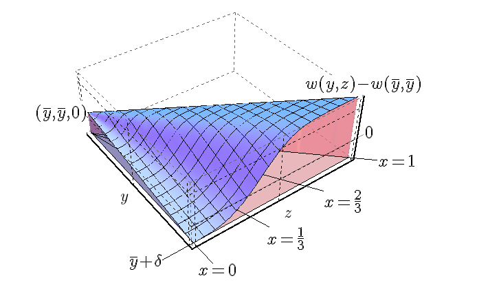
Figure 1: The surface representing $w(y,z)-w(\bar{y},\bar{y})$ in the neighborhood of the point $(y,z)=(\bar{y},\bar{y})$. This point appears in the left side of the picture, and the function takes the value 0 there. In the picture $y$ ranges from $\bar{y}$ to $\bar{y}+\delta$, and $z$ ranges from $\bar{y}$ to $y$. The parameter $x=(z-\bar{y})/(y-\bar{y})$ identifies directions in the $(y,z)$ plane, away from the point $(y,z)=(\bar{y},\bar{y})$, and biologically represents the fraction of individuals in the social environment of a mutant focal individual that are also mutants. The values of the directional derivatives $v(x)$, which represent marginal fitnesses, are indicated by the s-shaped curve produced by the intersection of the surface with the plane $y=\bar{y}+\delta$ (this s-shaped curve appears as the frontal border of the blue surface in the picture). The surface would only be well approximated by a plane, in the neighborhood of $(y,z)=(\bar{y},\bar{y})$, if $v(x)$ were a linear function, rather than s-shaped. Notice that $w$ is not differentiable anytime that $v(x)$ is a non-linear function of the fraction of mutant-types in the social environment; no kinks or discontinuities are necessary. When, as in this picture, differentiability at $(y,z)=(\bar{y},\bar{y})$ fails, one can not use the chain rule as in the derivation of (1), but the more general (4) still applies and provides the direction of selection.

References

- [1] Bowles, S., Gintis, H. (2011) A Cooperative Species: Human Reciprocity and its Evolution. (Princeton University Press, Princeton).
- [2] Boyd, R. and Richerson, P.J. (1988) The evolution of reciprocity in sizable groups. Journal of Theoretical Biology 132, 337-357.
- [3] Chuang, J.S., Rivoire, O. and Leibler, S. (2010) Cooperation and Hamilton’s rule in a simple microbial system. Molecular Systems Biology 6, 1-7.
- [4] Frank, S.A. (1998) Foundations of Social Evolution. (Princeton University Press, Princeton).
- [5] Gardner, A., West, S.A. and Wild, G. (2011) The genetical theory of kin selection. Journal of Evolutionary Biology 24, 1020-1043.
- [6] Gore, J., Youk, H. and van Oudenaarden, A. (2009) Snowdrift game dynamics and facultative cheating in yeast. Nature 459, 253-256.
- [7] Grafen, A. (1985) A geometric view of relatedness. Oxford Surveys in Evolutionary Biology 2, 28-90.
- [8] Hamilton, W.D. (1964) The genetical evolution of social behavior I and II. Journal of Theoretical Biology 7, 1-52.
- [9] Joshi, N.V. (1987) Evolution of cooperation by reciprocation within structured demes. Journal of Genetics 66, 69-84.
- [10] Kaplan, W. (1991) Advanced Calculus (4th edition). (Addison-Wesley, Reading, Mass.)
- [11] Lehmann, L. and Rousset, F. (2010) How life history and demography promote or inhibit the evolution of helping behaviors. Philosophical Transactions of the Royal Society B 365, 2599-2617.
- [12] Lessard, S. (2009) Diffusion approximations for one-locus multi-allele kin selection, mutation and random drift in group-structured populations: a unifying approach to selection models in population genetics. Journal of Mathematical Biology 59, 659-696.
- [13] Ohtsuki, H. (2010) Evolutionary games in Wright’s Island model: kin selection meets evolutionary game theory. Evolution 64, 3344-3353.
- [14] Rousset, F. (2004) Genetic Structure and Selection in subdivided populations. (Princeton University Press. Princeton).
- [15] Roze, D. and Rousset, F. (2008) Multilocus models in infinite island modedel of population structure. Theoretical Population Biology 73, 529-542.
- [16] Schonmann, R.H., Vicente, R. and Caticha, N. (2011) Altruism can proliferate through group/kin selection despite high random gene flow. Preprint.
- [17] Smith, J., Van Dyken, D. and Zee, P.C. (2010) A generalization of Hamilton’s rule for the evolution of microbial cooperation. Science 328, 1700-1703.
- [18] Taylor, P.D. and Frank, S.A. (1996) How to make a kin selection model. Journal of Theoretical Biology 180, 27-37.
- [19] Wenseleers, T., Gardner, A. and Foster, K. (2010) Social evolution theory: a review of methods and approaches. In: Social Behaviour: Genes, Ecology and Evolution. Szekely, T., Moore, A.J. and Komdeur, J., eds. (Cambridge University Press) 132-158.