Locally Linearized Runge Kutta method of Dormand and Prince

Abstract

In this paper, the effect that produces the local linearization of the embedded Runge-Kutta formulas of Dormand and Prince for initial value problems is studied. For this, embedded Locally Linearized Runge-Kutta formulas are defined and their performance is analyzed by means of exhaustive numerical simulations. For a variety of well-known physical equations with different dynamics, the simulation results show that the locally linearized formulas exhibit significant higher accuracy than the original ones, which implies a substantial reduction of the number of time steps and, consequently, a sensitive reduction of the overall computation cost of their adaptive implementation.

1 Introduction

It is well known (see, e.g., [3, 25, 21]) that conventional numerical schemes such as Runge-Kutta, Adams-Bashforth, predictor-corrector and others produce misleading dynamics when integrating Ordinary Differential Equations (ODEs). Typical problems are, for instance, the convergence to spurious steady states, changes in the basis of attraction, appearance of spurious bifurcations, etc. This might yield serious mistakes in the interpretation and analysis of the processes under consideration in practical control engineering or in applied sciences. The essence of such difficulties is that the dynamic of the numerical schemes (considered as discrete dynamical systems) is far richer than that of its continuous counterparts. Contrary to the popular belief, drawbacks of this type may no be solved by reducing the stepsize of the numerical method. Therefore, it is highly desirable the development of numerical integrators that preserve, as much as possible, the dynamical properties of the underlaying dynamical system for all step sizes or relative big ones. In this direction, some modest advances has been achieved by a number of relative recent integrators of the class of Exponential Methods, which are characterized by the explicit use of exponentials to obtain an approximate solution. An example of such integrators are the High Order Local Linearization (HOLL) methods based on Runge-Kutta schemes [4, 5, 13].

HOLL integrators are obtained by splitting, at each time step, the solution of the original ODE in two parts: the solution of a linear ODE plus the solution of an auxiliary ODE. The linear equation is solved by a Local Linearization (LL) scheme [14, 15] in such a way that A-stability is ensured, whereas the solution of the auxiliary one can be approximated by any conventional numerical integrator, preferably a high order explicit scheme. Originally, HOLL methods were introduced as a flexible approach for increasing the order of convergence of the order-$2$ LL method but, in addition, they can be thought as a strategy for constructing high order A-stable explicit schemes based on conventional explicit integrators. For this reason, if we focus on the conventional integrator involved in a particular HOLL scheme, then it is natural to say that the first one has been locally linearized. In this way, if a Runge Kutta scheme is used to approximate the above mentioned auxiliary ODE, the resulting HOLL scheme are indistinctly called Local Linearization - Runge Kutta (LLRK) scheme or Locally Linearized Runge Kutta (LLRK) scheme.

In [5], general results on the convergence, stability and dynamical properties of the Locally Linearized Runge Kutta method were studied. Specifically, it was demonstrated that: 1) the LLRK approach defines a general class of high order A-stable explicit integrators that preserve the convergence rate of the involved (not A-stable) explicit RK schemes; 2) in contrast with others A-stable explicit methods (such as Rosenbrock or the Exponential integrators), the RK coefficients involved in the LLRK integrators are not constrained by any stability condition and they just need to satisfy the usual, well-known order conditions of RK schemes, which makes the LLRK approach more flexible and simple; 3) LLRK integrators have a number of convenient dynamical properties such as the linearization preserving and the conservation of the exact solution dynamics around hyperbolic equilibrium points and periodic orbits; and 4) because of the flexibility in the numerical implementation of the LLRK discretizations, specific-purpose LLRK schemes can be designed for certain classes of ODEs, e.g., for moderate or large systems of equations. On the other hand, simulation studies carried out in [4, 5, 22] have shown that, for a variety of test equations, LLRK schemes of order $3$ and $4$ preserve much better the stability and dynamical properties of the actual solutions than their corresponding conventional RK schemes.

However, the accuracy and computational efficiency of the Local Linearization methods have been much less considered up to now, being the dynamical properties of such schemes the focus of previous studies and the main reason for the development of these methods. The few available results are the following. On an identical time partition [5], the LLRK scheme based on the classical order-$4$ RK scheme displays better accuracy than the order-$5$ RK formula of Dormand & Prince [7] in the integration of a variety of ODEs. On different time partitions [22], similar results are obtained by an adaptive implementation of the mentioned LLRK scheme in comparison with the Matlab code ode$45$, which provides an adaptive implementation of the embedded RK formulas of Dormand & Prince. However, this is achieved at expense of additional evaluations of the vector field, and with larger overall computational time. With this respect, the main drawback of that adaptive LLRK scheme is the absence of a computationally efficient strategy based on embedded formulas.

The main purpose of this work is introducing an adaptive LLRK scheme based on the embedded RK formulas of Dormand & Prince and evaluating, with simulations, its accuracy and computational efficiency in order to study the effect that the local linearization produces on these known RK formulas. The Matlab code developed with this goal is, same as the Matlab code ode$45$, addressed to low dimensional non stiff initial value problems for medium to low accuracies.

The paper is organized as follows. In the Section 2, a basic introduction on the Local Linearization - Runge Kutta (LLRK) schemes is presented. In the Section 3, the embedded Locally Linearized Runge-Kutta formulas are defined, and an adaptive implementation of them is described. In the last two sections, the results of a variety of exhaustive numerical simulations with well-known test equations are presented and discussed respectively.

2 Notations and preliminaries

Let $\mathcal{D}\subset\mathbb{R}^{d}$ be an open set. Consider the $d$-dimensional differential equation

$$\frac{d\mathbf{x}\left(t\right)}{dt} = \mathbf{f}\left(t,\mathbf{x}\left(t\right)\right)\text{, \ \ }t\in\left[t_{0},T\right]$$ (1)

$$\mathbf{x}(t_{0}) = \mathbf{x}_{0},$$ (2)

where $\mathbf{x}_{0}\in\mathcal{D}$ is a given initial point, and $\mathbf{f}:\left[t_{0},T\right]\times\mathcal{D}\longrightarrow\mathbb{R}^{d}$ is a differentiable function. Lipschitz and smoothness conditions on the function $\mathbf{f}$ are assumed in order to ensure a unique solution of this equation in $\mathcal{D}$.

Let $\left(t\right)_{h}=\left\{t_{n}:n=0,1,\ldots,N\right\}$ be a time discretization with maximum stepsize $h$ defined as a sequence of times that satisfy the conditions $t_{0}<t_{1}<\cdots<t_{N}=T$ and $\sup\limits_{n}(h_{n})\leq h<1$, where $h_{n}=t_{n+1}-t_{n}$ for $n=0,\ldots,N-1$.

For a given $(t_{n},\mathbf{y}_{n})$, let $\mathbf{v}_{n+1}=\mathbf{y}_{n}+\Lambda_{1}\left(t_{n},\mathbf{y}_{n};h_{n}\right)$ be an order-$\gamma_{1}$ approximation to solution of the linear ODE

$$\frac{d\mathbf{z}_{1}\left(t\right)}{dt} = \mathbf{B}_{n}\mathbf{z}_{1}(t)+\mathbf{b}_{n}\left(t\right)\mathbf{,}\text{ \ \ }t\in[t_{n},t_{n+1}],$$ (3)

$$\mathbf{z}_{1}\left(t_{n}\right) = \mathbf{y}_{n}$$ (4)

at $t_{n+1}$, and let $\mathbf{w}_{n+1}=\Lambda_{2}^{\mathbf{y}_{n}}\left(t_{n},\mathbf{0};h_{n}\right)$ be an order-$\gamma_{2}$ Runge-Kutta scheme approximating the solution of the nonlinear ODE

$$\frac{d\mathbf{z}_{2}\left(t\right)}{dt} = \mathbf{q}(t_{n},\mathbf{y}_{n};t\mathbf{,\mathbf{z}}_{2}\left(t\right)\mathbf{),}\text{ \ \ }t\in[t_{n},t_{n+1}],\quad$$ (5)

$$\mathbf{z}_{2}\left(t_{n}\right) = \mathbf{0}$$ (6)

at $t_{n+1}$, where $\mathbf{B}_{n}=\mathbf{f}_{\mathbf{x}}\left(t_{n},\mathbf{y}_{n}\right)$ is a $d\times d$ constant matrix, and

$$\mathbf{b}_{n}(t)=\mathbf{f}_{t}\left(t_{n},\mathbf{y}_{n}\right)(t-t_{n})+\mathbf{f}\left(t_{n},\mathbf{y}_{n}\right)-\mathbf{B}_{n}\mathbf{y}_{n}$$

and

$$\mathbf{q}(t_{n},\mathbf{y}_{n};s\mathbf{,\xi}) = \mathbf{f}(s,\mathbf{y}_{n}+\Lambda_{1}\left(t_{n},\mathbf{y}_{n};s-t_{n}\right)+\mathbf{\xi})-\mathbf{f}_{\mathbf{x}}(t_{n},\mathbf{y}_{n})\Lambda_{1}\left(t_{n},\mathbf{y}_{n};s-t_{n}\right)$$

$$-\mathbf{f}_{t}\left(t_{n},\mathbf{y}_{n}\right)(s-t_{n})-\mathbf{f}\left(t_{n},\mathbf{y}_{n}\right)$$

are $d$-dimensional vectors. Here, $\mathbf{f}_{x}$ and $\mathbf{f}_{t}$ denote the partial derivatives respect to $\mathbf{x}$ and $t$, respectively. Note that the vector field of the equation (5) not only depends on the point $(t_{n},\mathbf{y}_{n})$ but also of the numerical flow used to approximate $\mathbf{z}_{1}(t)$.

Definition 1

([4, 13, 5]) A Local Linearization - Runge Kutta (LLRK) scheme for the ODE (1)-(2) is defined by the recursive expression

$$\mathbf{y}_{n+1}=\mathbf{y}_{n}+\Lambda_{1}\left(t_{n},\mathbf{y}_{n};h_{n}\right)+\Lambda_{2}^{\mathbf{y}_{n}}\left(t_{n},\mathbf{0};h_{n}\right)$$ (7)

for all $t_{n}\in$ $\left(t\right)_{h}$, starting with $\mathbf{y}_{0}=\mathbf{x}_{0}$.

Local truncation error, rate of convergence and various dynamical properties of the general class of Local Linearization - Runge Kutta schemes (7) has been studied in [5].

According to the Definition 1, a variety of LLRK schemes can be derived. In previous works [4, 5] , the Local Linearization scheme based on Padé approximations [14, 15] has been used to integrate the linear ODE (3)-(4), whereas the so called four order classical Runge-Kutta scheme [2] has been applied to integrate the nonlinear ODE (5)-(6). This yields the order-$4$ LLRK scheme

$$\mathbf{y}_{n+1}=\mathbf{y}_{n}+\mathbf{u}_{4}+\frac{h_{n}}{6}(2\mathbf{k}_{2}+2\mathbf{k}_{3}+\mathbf{k}_{4}),$$ (8)

where

$$\mathbf{u}_{j}=\mathbf{L}(\mathbf{P}_{6,6}(2^{-\kappa_{j}}\mathbf{D}_{n}c_{j}h_{n}))^{2^{\kappa_{j}}}\mathbf{r}$$

and

$$\mathbf{k}_{j}=\mathbf{f}\left(t_{n}+c_{j}h_{n},\mathbf{y}_{n}+\mathbf{u}_{j}+c_{j}h_{n}\mathbf{k}_{j-1}\right)-\mathbf{f}\left(t_{n},\mathbf{y}_{n}\right)-\mathbf{f}_{\mathbf{x}}\left(t_{n},\mathbf{y}_{n}\right)\mathbf{u}_{j}\ -\mathbf{f}_{t}\left(t_{n},\mathbf{y}_{n}\right)c_{j}h_{n},$$

with $\mathbf{k}_{1}\equiv\mathbf{0}$ and $c=\left[\begin{array}[]{cccc}0&\frac{1}{2}&\frac{1}{2}&1\end{array}\right]$. Here, $\mathbf{P}_{p,q}(\cdot)$ denotes the $(p,q)$-Padé approximation for exponential matrices [18], and $\kappa_{j}$ the smallest integer number such that $\left\|2^{-\kappa_{j}}\mathbf{D}_{n}c_{j}h_{n}\right\|\leq\frac{1}{2}$. The matrices $\mathbf{D}_{n}$, $\mathbf{L}$ and $\mathbf{r}$ are defined as

$$\mathbf{D}_{n}=\left[\begin{array}[]{ccc}\mathbf{f}_{\mathbf{x}}(t_{n},\mathbf{y}_{n})&\mathbf{f}_{t}(t_{n},\mathbf{y}_{n})&\mathbf{f}(t_{n},\mathbf{y}_{n})\\ 0&0&1\\ 0&0&0\end{array}\right]\in\mathbb{R}^{(d+2)\times(d+2)},$$

$\mathbf{L}=\left[\begin{array}[]{ll}\mathbf{I}_{d}&\mathbf{0}_{d\times 2}\end{array}\right]$ and $\mathbf{r}^{\intercal}=\left[\begin{array}[]{ll}\mathbf{0}_{1\times(d+1)}&1\end{array}\right]$ for non-autonomous ODEs; and as

$$\mathbf{D}_{n}=\left[\begin{array}[]{cc}\mathbf{f}_{\mathbf{x}}(\mathbf{y}_{n})&\mathbf{f}(\mathbf{y}_{n})\\ 0&0\end{array}\right]\in\mathbb{R}^{(d+1)\times(d+1)},$$

$\mathbf{L}=\left[\begin{array}[]{ll}\mathbf{I}_{d}&\mathbf{0}_{d\times 1}\end{array}\right]$ and $\mathbf{r}^{\intercal}=\left[\begin{array}[]{ll}\mathbf{0}_{1\times d}&1\end{array}\right]$ for autonomous equations.

On an identical time partition [5], LLRK formula (8) displays better accuracy than the order-$5$ RK formula of Dormand & Prince in the integration of a variety of ODEs. On different time partitions [22], similar results are obtained by an adaptive implementation of LLRK formula (8) in comparison with the Matlab ode$45$ code, which provides an adaptive implementation of the embedded RK formulas of Dormand & Prince. However, this is achieved at expense of additional evaluations of the vector field $\mathbf{f}$, and with larger overall computational time. This cost can be sensitively reduced by using the $(2,2)$-Padé approximations instead of the order $(6,6)$ one used in formula (8), preserving the order of convergence and without significant lost of accuracy [22].

Local truncation error, rate of convergence, A-stability and various dynamical properties of the LLRK schemes based on Padé approximations has also been studied in [5].

For a precise comparison of the Local Linearization - Runge Kutta method with well-known integration methods such as Rosenbrock, Exponential Integrators, Splitting Methods and others, the interested reader might read [5] or [13].

3 Numerical scheme

3.1 Embedded Locally Linearized Runge-Kutta formulas

In view of the Definition 1, new integration formulas can be obtained as follows. Similarly to the LLRK scheme (8), the Local Linearization scheme based on Padé approximations [14, 15] is used for integrating the linear ODE (3)-(4) but, instead of the classical order-$4$ RK scheme, the embedded Runge-Kutta formulas of Dormand & Prince [7] is now applied to integrate the nonlinear ODE (5)-(6). This yields the embedded Locally Linearized Runge-Kutta formulas

$$\mathbf{y}_{n+1}=\mathbf{y}_{n}+\mathbf{u}_{s}+h_{n}\sum_{j=1}^{s}b_{j}\mathbf{k}_{j}\ \ \ \text{and}\ \ \ \ \ \widehat{\mathbf{y}}_{n+1}=\mathbf{y}_{n}+\mathbf{u}_{s}+h_{n}\sum_{j=1}^{s}\widehat{b}_{j}\mathbf{k}_{j},$$ (9)

where $s=7$ is the number of the stages,

$$\mathbf{u}_{j}=\mathbf{L}(\mathbf{P}_{p,q}(2^{-\kappa_{j}}\mathbf{D}_{n}c_{j}h_{n}))^{2^{\kappa_{j}}}\mathbf{r}$$ (10)

and

$$\mathbf{k}_{j}=\mathbf{f(}t_{n}+c_{j}h_{n},\mathbf{y}_{n}+\mathbf{u}_{j}+h_{n}\sum_{i=1}^{s-1}a_{j,i}\mathbf{k}_{i})-\mathbf{f}\left(t_{n},\mathbf{y}_{n}\right)-\mathbf{f}_{\mathbf{x}}\left(t_{n},\mathbf{y}_{n}\right)\mathbf{u}_{j}\ -\mathbf{f}_{t}\left(t_{n},\mathbf{y}_{n}\right)c_{j}h_{n},$$

with $\mathbf{k}_{1}\equiv\mathbf{0}$ and Runge-Kutta coefficients $a_{j,i}$, $b_{j}$, $\widehat{b}_{j}$ and $c_{j}$ defined in the Table 1. Here, $\mathbf{P}_{p,q}(\cdot)$ denotes the $(p,q)$-Padé approximation for exponential matrices with $p+q>4$. The number $\kappa_{j}$ and the matrices $\mathbf{D}_{n}$, $\mathbf{L}$ and $\mathbf{r}$ are defined as in the previous section.

0
$\frac{1}{5}$	$\frac{1}{5}$
$\frac{3}{10}$	$\frac{3}{40}$	$\frac{9}{40}$
$\frac{4}{5}$	$\frac{44}{45}$	$-\frac{56}{15}$	$\frac{32}{9}$
$\frac{8}{9}$	$\frac{19372}{6561}$	$-\frac{25360}{2187}$	$\frac{64448}{6561}$	$-\frac{212}{729}$
$1$	$\frac{9017}{3168}$	$-\frac{355}{33}$	$\frac{46732}{5247}$	$\frac{49}{176}$	$-\frac{5103}{18656}$
$1$	$\frac{35}{384}$	$0$	$\frac{500}{1113}$	$\frac{125}{192}$	$-\frac{2187}{6784}$	$\frac{11}{84}$
$y$	$\frac{35}{384}$	$0$	$\frac{500}{1113}$	$\frac{125}{192}$	$-\frac{2187}{6784}$	$\frac{11}{84}$	$0$
$\hat{y}$	$\frac{5179}{57600}$	$0$	$\frac{7571}{16695}$	$\frac{393}{640}$	$-\frac{92097}{339200}$	$\frac{187}{2100}$	$\frac{1}{40}$

Table 1: Coefficients tableau for the embedded formulas.

The local truncation error, the rate of convergence and the A-stability of the LLRK formulas (9) will be consider in what follows. With this purpose, these formulas are rewritten as

$$\mathbf{y}_{n+1}=\mathbf{y}_{n}+h_{n}\varphi(t_{n,}\mathbf{y}_{n};h_{n})\text{\ \ \ \ \ \ \ \ \ and \ \ \ \ \ \ \ \ \ \ \ }\widehat{\mathbf{y}}_{n+1}=\mathbf{y}_{n}+h_{n}\widehat{\varphi}(t_{n,}\mathbf{y}_{n};h_{n})\text{,}$$

and the following additional notations are introduced. Let $\mathcal{D}$ be an open subset of $\mathbb{R}^{d}$, $\mathcal{M}$ an upper bound for $\left\|\mathbf{f}_{\mathbf{x}}\right\|$ on $[t_{0},T]\times\mathcal{D}$, and $\mathcal{L}$ the Lipschitz constant of the function $q(t,x(t);\cdot)$ (which exists for all $t\in[t_{0},T]$ because Lemma 6 in [5] under regular conditions for $\mathbf{f}$). Denote by $L_{n+1}$ the local truncation error of the Local Linearization scheme $\mathbf{y}_{n+1}=\mathbf{y}_{n}+u_{4}$ when it is applied to the linear equation (3)-(4), for which the inequality

$$L_{n+1}\leq Ch^{p+q+1}$$

holds with positive constant $C$ [15]. Further, denote by $L_{n+1}^{1}$ and $L_{n+1}^{2}$ the local truncation errors of the classical embedded Runge-Kutta formulas of Dormand and Prince when they are applied to the nonlinear equation (5)-(6), for which the inequalities

$$L_{n+1}^{1}\leq C_{1}h^{6}\text{\ \ \ \ \ \ \ \ \ and \ \ \ \ \ \ \ \ \ \ \ }L_{n+1}^{2}\leq C_{2}h^{5}$$

hold with positive constants $C_{1}$ and $C_{2}$ [7, 8].

Theorem 1

Let $\mathbf{x}$ be the solution of the ODE (1)-(2) with vector field $\mathbf{f}$ six times continuously differentiable on $[t_{0},T]\times\mathcal{D}$. Then, the embedded Locally Linearized Runge-Kutta formulas (9) have local truncation errors

$$\left\|\mathbf{x}(t_{n+1})-\mathbf{x}(t_{n})-h_{n}\varphi(t_{n,}\mathbf{x}(t_{n});h_{n})\right\|\leq Kh_{n}^{p+q+1}+C_{1}h_{n}^{6}$$

and

$$\left\|\mathbf{x}(t_{n+1})-\mathbf{x}(t_{n})-h_{n}\widehat{\varphi}(t_{n,}\mathbf{x}(t_{n});h_{n})\right\|\leq Kh_{n}^{p+q+1}+C_{2}h_{n}^{5};$$

and global errors

$$\left\|\mathbf{x}(t_{n+1})-\mathbf{y}_{n+1}\right\|\leq M_{1}h^{\min\{p+q,5\}}$$

and

$$\left\|\mathbf{x}(t_{n+1})-\widehat{\mathbf{y}}_{n+1}\right\|\leq M_{2}h^{\min\{p+q,4\}}$$

for all $t_{n+1}\in\left(t\right)_{h}$ and $h$ small enough, where $K=C(1+\frac{\mathcal{M}}{\mathcal{L}}(e^{\mathcal{L}}-1))$ is a positive constant, and $M_{1}$ and $M_{2}$ as well. In addition, the embedded Locally Linearized Runge-Kutta formulas (9) are A-stable if in the involved $(p,q)$-Padé approximation the inequality $p\leq q\leq p+2$ holds.

Proof. The local truncation errors and the global errors are a straightforward consequence of Theorem 15 in [5], whereas the A-stability is a direct result of Theorem 17 in [5]. $\square$

Clearly, according to this result, the Locally Linearized Runge-Kutta formulas (9) preserve the convergence rate of the classical embedded Runge-Kutta formulas of Dormand and Prince if the inequality $p+q>4$ holds. Further, note that these Locally Linearized formulas not only preserve the stability of the linear ODEs when $p\leq q\leq p+2$, but they are also able to "exactly" (up to the precision of the floating-point arithmetic) integrate this class of equations when $p+q=12$ (for the numerical precision of the current personal computers [18]).

In addition, and trivially, the embedded Locally Linearized Runge-Kutta formulas (9) inherit the dynamical properties derived in [5] for the general class of Local Linearization - Runge Kutta methods.

3.2 Adaptive strategy

In order to write a code that automatically adjust the stepsizes for achieving a prescribed tolerance of the local error at each step, an adequate adaptive strategy is necessary. At glance, the automatic stepsize control for the embedded RK formulas of Dormand & Prince seems to fit well for the embedded LLRK formulas (9). In what follows, the adaptive strategy of the Matlab code ode$45$ for these formulas is described.

Once the values for the relative and absolute tolerances $RTol$ and $ATol$, and for the maximum and minimum stepsizes $h_{\max}$ and $h_{\min}$ are set, the basic steps of the algorithm are:

1. Estimation of the initial stepsize

   $$h_{0}=\min\{h_{\max},\max\{h_{\min},\Delta\}\}$$

   where

   $$\Delta=\left\{\begin{array}[]{cc}\frac{1}{r_{h}}&\text{if }h_{max}\cdot r_{h}>1\\ h_{\max}&\text{otherwise}\end{array}\right.$$

   with

   $$r_{h}=\frac{1}{0.8\cdot RTol^{1/5}}\max_{i=1...d}\left\{\frac{\mathbf{f}^{i}(\mathbf{y}_{0})}{\max\left\{|\mathbf{y}_{0}^{i}|,tr\right\}}\right\}$$

   and $tr=$ $\frac{ATol}{RTol}$. Initialize $fail=0$.

2. Evaluation of the embedded formula (9)

3. Estimation of the error

   $$error={\LARGE||}\frac{\mathbf{y}_{n+1}-\widehat{\mathbf{y}}_{n+1}}{\underset{i=1,\ldots,d}{\max}\left\{|\mathbf{y}_{n}^{i}|,|\ \mathbf{y}_{n+1}^{i}|,tr\right\}}{\LARGE||}_{\infty}$$

4. Estimation of a new stepsize

   $$h_{new}=\min\{h_{\max},\max\{h_{\min},\Delta\}\}$$

   where

   $$\Delta=\left\{\begin{array}[]{cc}0.8\cdot{\large(}\frac{RTol}{error}{\large)}^{1/5}\cdot h&\text{if }error\leq RTol\\ \max\{0.1,0.8\cdot{\large(\frac{RTol}{error})}^{1/5}\}\cdot h&\text{if }error>RTol\text{ and }fail=0\\ 0.5\cdot h&\text{if }error>RTol\text{ and }fail=1\end{array}\right.$$

5. Validation of $y_{n+1}$: if $error\leq RTol$, then accept $y_{n+1}$ as an approximation to $\mathbf{x}$ at $t_{n+1}=t_{n}+h$. Otherwise, return to 2 with $h_{n}=h_{new}$ and $fail=1.$

6. Control of the final step: if $t_{n}+h=T$, stop. If $t_{n}+h+h_{new}>T$, then redefine $h_{new}=T-(t_{n}+h)$.

7. Return to 2 with $n=n+1$, $h_{n}=h_{new}$, and $fail=0$.

3.3 Continuous formula

Continuous formulas of RK methods are usually defined for computing the solutions on a dense set of time instants with minimum computational cost. Typically [8], they are constructing by means of a polynomial interpolation of the RK formulas between two consecutive times $t_{n},t_{n+1}\in$ $\left(t\right)_{h}$.

By a simple combination of the LLRK formulas (9) with the continuous formulas of the Dormand & Prince RK method [8] for (5)-(6), a continuous $7$-stage LLRK formula can be defined as

$$\mathbf{y}(t_{n}+\theta h_{n})=\mathbf{y}_{n}+\mathbf{u}(\theta h_{n})+h_{n}\sum_{j=1}^{7}b_{j}(t_{n}+\theta h_{n})\mathbf{k}_{j}\ ,\ \ 0<\theta<1,$$ (11)

for all $t_{n},t_{n+1}\in$ $\left(t\right)_{h}$, where

$$\mathbf{u}(\theta h_{n})=\mathbf{L}(\mathbf{P}_{p,q}(2^{-\kappa_{j}}\mathbf{D}_{n}\theta h_{n}))^{2^{\kappa_{j}}}\mathbf{r}$$ (12)

is a $d$-dimensional vector, and

$$b_{j}(\delta)=\sum\limits_{i=1}^{4}\alpha_{i,j}\delta^{i}$$

is a polynomial with coefficients $\alpha_{i,j}$. Here, the function $\mathbf{k}_{j}$, the matrices $\mathbf{D}_{n}$, $\mathbf{L}$ and $\mathbf{r}$, and the number $\kappa_{j}$ are defined as in (9), as well as the $(p,q)$-Padé approximation $\mathbf{P}_{p,q}$. The coefficients $\alpha_{i,j}$, defined in Table 2, coincide with those of the continuous RK formula implemented in the Matlab code ode$45$.

$j/i$ $1$ $2$ $3$ $4$ $1$ $1$ $-183/64$ $37/12$ $-145/128$ $2$ $0$ $0$ $0$ $0$ $3$ $0$ $1500/371$ $-1000/159$ $1000/371$ $4$ $0$ $-125/32$ $125/12$ $-375/64$ $5$ $0$ $9477/3392$ $-729/106$ $25515/6784$ $6$ $0$ $-11/7$ $11/3$ $-55/28$ $7$ $0$ $3/2$ $-4$ $5/2$

Table 2: Values of the coefficient $\alpha_{i,j}$ involved in the continuous LLRK formula (11) .

3.4 LLDP45 code

This subsection describes a Matlab2007b(32bits) implementation of the adaptive scheme described above, which will be denoted as LLDP$45$ code.

In order to make a fair comparison between the linearized and the nonlinearized RK formulas, the LLDP$45$ code is an exact copy of the ode$45$ one with the exception of the program lines corresponding to the embedded and continuous formulas of Dormand and Prince, which are replaced by the formulas (9) and (11) respectively. We recall that the code ode$45$ implements the adaptive strategy of the subsection 3.2 for the embedded RK formulas of Dormand & Prince, which is considered by many authors the most recommendable code to be applied as first try for most problems [19].

Note that, the embedded LLRK formulas (9) require the computation of six Padé approximations $\mathbf{P}_{p,q}$ at each integration step, which increases the computational cost of the original embedded RK formulas. Nevertheless, this number of Padé approximations can be reduced by taking in to account that: a) $(\mathbf{P}_{p,q}(2^{-\kappa}\mathbf{D}_{n}c_{j}h_{n}))^{2^{\kappa}}$ gives an approximation to exponential matrix $\mathbf{e}^{\mathbf{D}_{n}c_{j}h_{n}}$; and b) the flow property of the exponential operator. Indeed, this can be carried out in two steps:

1. approximating $\mathbf{e}^{\mathbf{D}_{n}h_{n}/90}$ by the matrix $\mathbf{M}_{1/90}=$ $(\mathbf{P}_{p,q}(2^{-\kappa}\mathbf{D}_{n}h_{n}/90))^{2^{\kappa}},$ where $\kappa$ is the smallest integer number such that $\left\|2^{-\kappa}\mathbf{D}_{n}h_{n}/90\right\|\leq\frac{1}{2}$; and

2. the successive computation of the matrices

   $$\mathbf{M}_{2/90} = \mathbf{M}_{1/90}\mathbf{M}_{1/90}\ \ \ \ \ \ \ \ \ \mathbf{M}_{4/90}=\mathbf{M}_{2/90}\mathbf{M}_{2/90}$$

   $$\mathbf{M}_{8/90} = \mathbf{M}_{4/90}\mathbf{M}_{4/90}\ \ \ \ \ \ \ \ \mathbf{M}_{16/90}=\mathbf{M}_{8/90}\mathbf{M}_{8/90}$$

   $$\mathbf{M}_{32/90} = \mathbf{M}_{16/90}\mathbf{M}_{16/90}\ \ \ \ \ \ \mathbf{M}_{80/90}=\mathbf{M}_{32/90}\mathbf{M}_{16/90}\mathbf{M}_{32/90}$$

   $$\mathbf{M}_{1/10} = \mathbf{M}_{8/90}\mathbf{M}_{1/90}\ \ \ \ \ \ \ \ \ \ \ \mathbf{M}_{1/5}=\mathbf{M}_{1/10}\mathbf{M}_{1/10}$$

   $$\mathbf{M}_{2/5} = \mathbf{M}_{1/5}\mathbf{M}_{1/5}\ \ \ \ \ \ \ \ \ \ \ \ \ \ \mathbf{M}_{4/5}=\mathbf{M}_{2/5}\mathbf{M}_{2/5}$$

   $$\mathbf{M}_{3/10} = \mathbf{M}_{1/10}\mathbf{M}_{1/5}\ \ \ \ \ \ \ \ \ \ \ \ \ \ \ \mathbf{M}_{1}=\mathbf{M}_{4/5}\mathbf{M}_{1/5}.$$

Consequently, the matrix $\mathbf{M}_{c_{j}}$ corresponding to each RK coefficient $c_{j}$ provides an approximation to $\mathbf{e}^{\mathbf{D}_{n}c_{j}h_{n}}$, for all $j=1,..,6$. In this way, at each integration step, the code LLDP$45$ performs six evaluation of $\mathbf{f}$ (same than the ode$45$ code), one Jacobian matrix and one matrix exponential.

The matrix $\mathbf{M}_{1/90}$ is computed by means of the function "expmf", which provides a C++ implementation of the classical $(p,q)$-Padé approximations algorithm for exponential matrices with scaling and squaring strategy [18], and $p=q=3$.

4 Numerical simulations

In this section, the performance of the LLDP$45$ and ode$45$ codes is compared by means of numerical simulations. To do so, a variety of ODEs and simulation types were selected. For all of them, the Relative Error

$$RE=\underset{{\small i=1,\ldots,d;}\text{ }{\small t}_{j}{\small\in(t)}_{h}}{\max}\left|\frac{\mathbf{x}^{i}(t_{j})-\mathbf{y}^{i}(t_{j})}{\mathbf{x}^{i}(t_{j})}\right|$$ (13)

between the "exact" solution $\mathbf{x}$ and its approximation $\mathbf{y}$ is evaluated.

The simulations with the code ode$45$ were carried out with a wide range of tolerances: crude with $RTol=10^{-3}$ and $ATol=10^{-6}$, mild with $RTol=10^{-6}$ and $ATol=10^{-9}$, and refined with $RTol=10^{-9}$ and $ATol=10^{-12}$. The Matlab code ode$15s$ with refined tolerance $RTol=10^{-13}$ and $ATol=10^{-13}$ was used to compute the "exact" solution $\mathbf{x}$ in all simulations.

4.1 Test examples

The first four examples have the semi-lineal form

$$\frac{d\mathbf{x}}{dt}=\mathbf{Ax+g}(\mathbf{x),}$$ (14)

where $\mathbf{A}$ is a square matrix and $\mathbf{g}$ is a function of $\mathbf{x}$. The vector field of the first two examples have Jacobian with eigenvalues on or near the imaginary axis, which made these equations difficult to be integrated by conventional schemes [19]. The other two are also hard for conventional explicit schemes since they are examples of stiff equations [19]. Example 4 has an additional complexity for a number of integrators that do not update the Jacobian of the vector field at each integration step [19, 12]: the Jacobian of the linear term has positive eigenvalues, which results a problem for the integration in a neighborhood of the stable equilibrium point $\mathbf{x}=1$.

Example 1

Periodic linear [5]

$$\frac{d\mathbf{x}}{dt}=\mathbf{A}(\mathbf{x}+2),$$

with

$$\mathbf{A}=\left[\begin{array}[]{cc}i&0\\ 0&-i\end{array}\right],$$

$\mathbf{x}(t_{0})=(-2.5,-1.5)$ and $[t_{0},T]=[0,4\pi]$.

Example 2

Periodic linear plus nonlinear term [5]

$$\frac{d\mathbf{x}}{dt}=\mathbf{A}(\mathbf{x}+2)+0.1\mathbf{x}^{2},$$

where the matrix $\mathbf{A}$ is defined as in the previous example, $\mathbf{x}(t_{0})=(1,1)$, and $[t_{0},T]=[0,4\pi]$.

Example 3

Stiff linear [5]

$$\frac{d\mathbf{x}}{dt}=-100\mathbf{H}(\mathbf{x+1}),$$

where $\mathbf{H}$ is the 12-dimensional Hilbert matrix (with conditioned number $1.69\times 10^{16}$), $\mathbf{x}^{i}(t_{0})=1$, $i=1\ldots 12$, and $[t_{0},T]=[0,1].$

Example 4

Stiff linear plus nonlinear term  [5]

$$\frac{d\mathbf{x}}{dt}=100\mathbf{H}(\mathbf{x}-\mathbf{1})+100(\mathbf{x}-\mathbf{1})^{2}-60(\mathbf{x}^{3}-\mathbf{1}),$$

where $\mathbf{H}$ is the 12-dimensional Hilbert matrix, $\mathbf{x}^{i}(t_{0})=-0.5$, $i=1\ldots 12$, and $[t_{0},T]=[0,1]$.

The following examples are well known nonlinear test equations. This include highly oscillatory, non stiff and mild stiff equations.

Example 5

Fermi–Pasta–Ulam equation defined by the Hamiltonian system [10]

$$H(\mathbf{p,q})=\frac{1}{2}\sum\limits_{i=1}^{3}(\mathbf{p}_{2i-1}^{2}+\mathbf{p}_{2i}^{2})+\frac{w^{2}}{4}\sum\limits_{i=1}^{3}(\mathbf{q}_{2i}-\mathbf{q}_{2i-1})^{2}+\sum\limits_{i=0}^{3}(\mathbf{q}_{2i+1}-\mathbf{q}_{2i})^{2}$$

with $w=50$, initial conditions $1,1,1/w,1$ for the four first variables and zero for the remainder eight, and $[t_{0},T]=[0,15].$

Example 6

Brusselator equation [8]:

$$\frac{dx_{1}}{dt} = 1+{\normalsize x}_{1}^{2}x_{2}-4x_{1}$$

$$\frac{dx_{2}}{dt} = 3x_{1}-x_{1}^{2}x_{2},$$

where $(x_{1}(t_{0}),x_{2}(t_{0}))=(1.5{\normalsize,3)}$ and $[t_{0},T]=[0,20]$.

Example 7

Rigid body equation [8]:

$$\frac{d{\normalsize x}_{1}}{dt} = {\normalsize x}_{2}x_{3}$$

$$\frac{d{\normalsize x}_{2}}{dt} = -{\normalsize x}_{1}x_{3}$$

$$\frac{d{\normalsize x}_{3}}{dt} = -0.51x_{1}{\normalsize x}_{2}$$

with $(x_{1}(t_{0}),x_{2}(t_{0}),x_{3}(t_{0}))=(0,1,1)$ over $[t_{0},T]=[0,12]$.

Example 8

Chemical reaction [19]:

$$\frac{d{\normalsize x}_{1}}{dt} = 1.3(x_{3}-x_{1})+10400k({\normalsize x}_{1}){\normalsize x}_{2}$$

$$\frac{d{\normalsize x}_{2}}{dt} = 1880(x_{4}-x_{2}(1+k({\normalsize x}_{1})\mathbf{))}$$

$$\frac{d{\normalsize x}_{3}}{dt} = 1752-269x_{3}+267x_{1}$$

$$\frac{d{\normalsize x}_{4}}{dt} = 0.1+320x_{2}-321x_{4}$$

where $k({\normalsize x_{1})=e^{(20.7-\frac{1500}{x_{1}})}}$. With initial condition $(50,0,600,0.1)$ over $[t_{0},T]=[0,1]$, this is mild stiff equation.

Example 9

Van der Pol equation [9]:

$$\frac{d{\normalsize x}_{1}}{dt} = x_{2}$$

$$\frac{d{\normalsize x}_{2}}{dt} = \varepsilon(1-x_{2}^{2})x_{1}+x_{2}$$

with $(x_{1}(t_{0}),x_{2}(t_{0}))=(2,0)$. With $\varepsilon=1$ and $\varepsilon=10^{2}$, this is a non stiff and a mild stiff equation on the intervals $[t_{0},T]=[0,20]$ and $[t_{0},T]=[0,300]$, respectively.

As illustration, Figure 1 shows the first component of the solution of each example, which will be consecutively named as PerLin, PerNoLin, StiffLin, StiffNoLin, fpu, bruss, rigid, chm, vdp1 and vdp100.

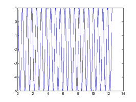
PerLin

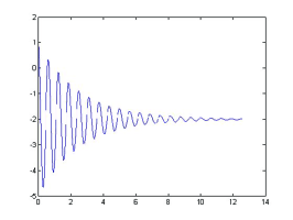
PerNoLin

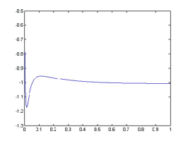
StiffLin

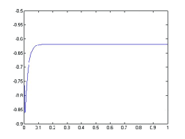
StiffNoLin

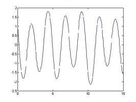
fpu

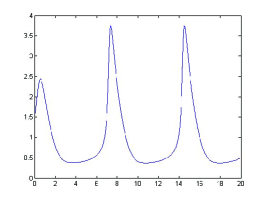
bruss

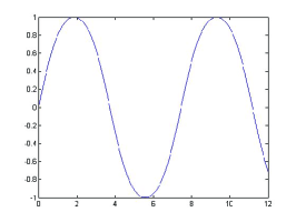
rigid

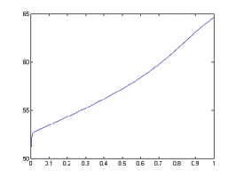
chm

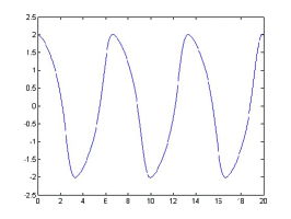
vdp1

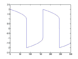
vdp100

Figure 1: Path of the first components of the solution in each example.

4.2 Simulation A: integration over same time partition

This simulation is designed to compare the accuracy of the order-$5$ formulas of the codes LLDP$45$ and ode$45$ over identical time partitions. First, the ode$45$ code integrates all the examples with the crude tolerances $RTol=10^{-3}$ and $ATol=10^{-6}$. This defined, for each example, a time partition $(t)_{h}$ over which the order-$5$ formula of the LLDP$45$ code is evaluated as well. That is, the formula

$$\mathbf{y}_{n+1}=\mathbf{y}_{n}+\mathbf{u}_{s}+h_{n}\sum_{j=1}^{s}b_{j}\mathbf{k}_{j}$$ (15)

with $\mathbf{u}_{j}=\mathbf{L}(\mathbf{P}_{3,3}(2^{-\kappa_{j}}\mathbf{D}_{n}c_{j}h_{n}))^{2^{\kappa_{j}}}\mathbf{r}$ for the LLDP$45$ code. Tables 3 and 4 present, respectively, the Relative Error (13) of the order-$5$ formula of each code in the integration of the four semilinear and six nonlinear examples defined above. The number of accepted time steps is shown as well. This comparison is repeated twice but with the mild and refined tolerances $RTol=10^{-6}$,$ATol=10^{-9}$ and $RTol=10^{-9}$,$ATol=10^{-12}$. The results are also shown in Tables 3 and 4.

Example Tol $\begin{array}[]{c}\text{Time}\\ \text{steps}\end{array}$ $\begin{array}[]{c}\text{Relative Error}\\ \text{DP formulas}\end{array}$ $\begin{array}[]{c}\text{Relative Error}\\ \text{LLDP formulas}\end{array}$ PerLin $\begin{array}[]{c}\text{Crude}\\ \text{Mild}\\ \text{Refined}\end{array}$ $\begin{array}[]{c}147\\ 598\\ 2394\end{array}$ $\begin{array}[]{c}1.01\\ 2.6\times 10^{-2}\\ 2.7\times 10^{-5}\end{array}$ $\begin{array}[]{c}2.0\times 10^{-6}\\ 3.2\times 10^{-7}\\ 1.3\times 10^{-6}\end{array}$ PerNoLin $\begin{array}[]{c}\text{Crude}\\ \text{Mild}\\ \text{Refined}\end{array}$ $\begin{array}[]{c}105\\ 411\\ 1634\end{array}$ $\begin{array}[]{c}1.3\times 10^{-2}\\ 2.6\times 10^{-5}\\ 1.2\times 10^{-7}\end{array}$ $\begin{array}[]{c}4.9\times 10^{-5}\\ 6.9\times 10^{-8}\\ 1.4\times 10^{-9}\end{array}$ StiffLin $\begin{array}[]{c}\text{Crude}\\ \text{Mild}\\ \text{Refined}\end{array}$ $\begin{array}[]{c}60\\ 78\\ 173\end{array}$ $\begin{array}[]{c}1.1\times 10^{-3}\\ 1.1\times 10^{-6}\\ 8.0\times 10^{-10}\end{array}$ $\begin{array}[]{c}2.7\times 10^{-12}\\ 2.7\times 10^{-12}\\ 2.7\times 10^{-12}\end{array}$ StiffNoLin $\begin{array}[]{c}\text{Crude}\\ \text{Mild}\\ \text{Refined}\end{array}$ $\begin{array}[]{c}104\\ 133\\ 294\end{array}$ $\begin{array}[]{c}1.4\times 10^{-2}\\ 1.5\times 10^{-5}\\ 1.4\times 10^{-8}\end{array}$ $\begin{array}[]{c}9.7\times 10^{-5}\\ 6.8\times 10^{-8}\\ 1.3\times 10^{-8}\end{array}$

Table 3: Relative error of the order-5 formula of each code when integrate the semilinear examples over identical time partition.

Note that, in general, the ode$45$ code is able to adequately integrate the test equations with the tree specified tolerances. Exceptions are the highly oscillatory fpu equation and the moderate stiff equation vpd100 at crude tolerances, for which the relative error is high or unacceptable, respectively. Observe that, the order-$5$ locally linearized formula (15) is able to integrate the first equation with an adequate relative error, but fail to integrate the second one on the time partition generated by the ode$45$ code. In this last case, the Pad algorithm fails to compute the exponential matrix at some point of the mentioned time partition and, because of that, the place corresponding to this information in Table 4 is empty.

Example Tol $\begin{array}[]{c}\text{Time}\\ \text{steps}\end{array}$ $\begin{array}[]{c}\text{Relative Error}\\ \text{DP formulas}\end{array}$ $\begin{array}[]{c}\text{Relative Error}\\ \text{LLDP formulas}\end{array}$ fpu $\begin{array}[]{c}\text{Crude}\\ \text{Mild}\\ \text{Refined}\end{array}$ $\begin{array}[]{c}964\\ 4474\\ 19190\end{array}$ $\begin{array}[]{c}1.9\times 10^{2}\\ 8.1\\ 1.7\times 10^{-2}\end{array}$ $\begin{array}[]{c}1.5\times 10^{-2}\\ 2.9\times 10^{-3}\\ 1.7\times 10^{-2}\end{array}$ rigid $\begin{array}[]{c}\text{Crude}\\ \text{Mild}\\ \text{Refined}\end{array}$ $\begin{array}[]{c}19\\ 66\\ 256\end{array}$ $\begin{array}[]{c}2.7\times 10^{-2}\\ 7.5\times 10^{-5}\\ 2.0\times 10^{-7}\end{array}$ $\begin{array}[]{c}1.5\times 10^{-3}\\ 4.0\times 10^{-6}\\ 1.8\times 10^{-8}\end{array}$ chm $\begin{array}[]{c}\text{Crude}\\ \text{Mild}\\ \text{Refined}\end{array}$ $\begin{array}[]{c}679\\ 723\\ 1520\end{array}$ $\begin{array}[]{c}1.1\times 10^{-3}\\ 1.1\times 10^{-6}\\ 1.2\times 10^{-8}\end{array}$ $\begin{array}[]{c}5.5\times 10^{-7}\\ 2.5\times 10^{-7}\\ 1.2\times 10^{-8}\end{array}$ bruss $\begin{array}[]{c}\text{Crude}\\ \text{Mild}\\ \text{Refined}\end{array}$ $\begin{array}[]{c}46\\ 148\\ 558\end{array}$ $\begin{array}[]{c}7.7\times 10^{-2}\\ 8.7\times 10^{-6}\\ 1.5\times 10^{-8}\end{array}$ $\begin{array}[]{c}2.4\times 10^{-2}\\ 3.5\times 10^{-7}\\ 1.2\times 10^{-9}\end{array}$ vdp1 $\begin{array}[]{c}\text{Crude}\\ \text{Mild}\\ \text{Refined}\end{array}$ $\begin{array}[]{c}59\\ 204\\ 785\end{array}$ $\begin{array}[]{c}2.0\\ 2.8\times 10^{-4}\\ 5.6\times 10^{-7}\end{array}$ $\begin{array}[]{c}0.14\\ 1.5\times 10^{-5}\\ 3.1\times 10^{-8}\end{array}$ vdp100 $\begin{array}[]{c}\text{Crude}\\ \text{Mild}\\ \text{Refined}\end{array}$ $\begin{array}[]{c}16916\\ 17516\\ 31254\end{array}$ $\begin{array}[]{c}1.9\times 10^{4}\\ 0.42\\ 1.2\times 10^{-3}\end{array}$ $\begin{array}[]{c}-\\ 9.2\times 10^{-2}\\ 8.1\times 10^{-4}\end{array}$

Table 4: Relative error of the order-5 formula of each code when integrate the nonlinear examples over identical time partition.

4.3 Simulation B: integration with same tolerance

This simulation is designed to compare the performance the codes LLDP$45$ and ode$45$ with the same tolerances. As a difference with Simulation A, here each codes use a different time partition defined by their own adaptive strategy.

Tables 5 and 6 summarize the results of each code in the integration of each example for the three sets of tolerances specified above. The column "Time" in these tables presents the relative overall time of each numerical scheme with respect to that of the ode45 code on the whole interval $[t_{0},T]$. This overall time ratio works as simple indicator to compare the total computational cost of each code. In addition, the tables show the number of accepted and failed steps, the number of evaluations of $\mathbf{f}$ and $\mathbf{f}_{x}$, and the number of exponential matrices computed in the integration of each example.

Example Code Tol $\begin{array}[]{c}\text{Time}\\ \text{steps}\end{array}$ $\begin{array}[]{c}\text{Failed}\\ \text{steps}\end{array}$ $f$ exp($f_{x})$ Time $\begin{array}[]{c}\text{Relative}\\ \text{Error}\end{array}$ PerLin ode45 $\begin{array}[]{c}\text{Crude}\\ \text{Mild}\\ \text{Refined}\end{array}$ $\begin{array}[]{c}147\\ 598\\ 2394\end{array}$ $\begin{array}[]{c}0\\ 0\\ 0\end{array}$ $\begin{array}[]{c}883\\ 3589\\ 14365\end{array}$ $\begin{array}[]{c}0\\ 0\\ 0\end{array}$ $\begin{array}[]{c}1\\ 1\\ 1\end{array}$ $\begin{array}[]{c}10.2\\ 2.6\times 10^{-2}\\ 2.7\times 10^{-5}\end{array}$ LLDP$45$ $\begin{array}[]{c}\text{Crude}\\ \text{Mild}\\ \text{Refined}\end{array}$ $\begin{array}[]{c}14\\ 14\\ 15\end{array}$ $\begin{array}[]{c}0\\ 0\\ 0\end{array}$ $\begin{array}[]{c}85\\ 85\\ 91\end{array}$ $\begin{array}[]{c}14\\ 14\\ 15\end{array}$ $\begin{array}[]{c}0.27\\ 0.08\\ 0.01\end{array}$ $\begin{array}[]{c}2.0\times 10^{-9}\\ 3.0\times 10^{-9}\\ 2.0\times 10^{-9}\end{array}$ PerNoLin ode45 $\begin{array}[]{c}\text{Crude}\\ \text{Mild}\\ \text{Refined}\end{array}$ $\begin{array}[]{c}105\\ 411\\ 1634\end{array}$ $\begin{array}[]{c}0\\ 0\\ 0\end{array}$ $\begin{array}[]{c}631\\ 2467\\ 9805\end{array}$ $\begin{array}[]{c}0\\ 0\\ 0\end{array}$ $\begin{array}[]{c}1\\ 1\\ 1\end{array}$ $\begin{array}[]{c}1.3\times 10^{-2}\\ 2.6\times 10^{-5}\\ 1.2\times 10^{-7}\end{array}$ LLDP$45$ $\begin{array}[]{c}\text{Crude}\\ \text{Mild}\\ \text{Refined}\end{array}$ $\begin{array}[]{c}42\\ 137\\ 534\end{array}$ $\begin{array}[]{c}0\\ 0\\ 0\end{array}$ $\begin{array}[]{c}253\\ 823\\ 3205\end{array}$ $\begin{array}[]{c}42\\ 137\\ 534\end{array}$ $\begin{array}[]{c}0.74\\ 0.62\\ 0.57\end{array}$ $\begin{array}[]{c}2.2\times 10^{-3}\\ 3.6\times 10^{-6}\\ 2.1\times 10^{-9}\end{array}$ StiffLin ode45 $\begin{array}[]{c}\text{Crude}\\ \text{Mild}\\ \text{Refined}\end{array}$ $\begin{array}[]{c}60\\ 78\\ 172\end{array}$ $\begin{array}[]{c}6\\ 1\\ 6\end{array}$ $\begin{array}[]{c}397\\ 475\\ 1069\end{array}$ $\begin{array}[]{c}0\\ 0\\ 0\end{array}$ $\begin{array}[]{c}1\\ 1\\ 1\end{array}$ $\begin{array}[]{c}1.1\times 10^{-3}\\ 1.1\times 10^{-6}\\ 8.0\times 10^{-10}\end{array}$ LLDP$45$ $\begin{array}[]{c}\text{Crude}\\ \text{Mild}\\ \text{Refined}\end{array}$ $\begin{array}[]{c}14\\ 14\\ 15\end{array}$ $\begin{array}[]{c}0\\ 0\\ 0\end{array}$ $\begin{array}[]{c}85\\ 85\\ 91\end{array}$ $\begin{array}[]{c}14\\ 14\\ 15\end{array}$ $\begin{array}[]{c}0.33\\ 0.34\\ 0.15\end{array}$ $\begin{array}[]{c}2.5\times 10^{-12}\\ 2.3\times 10^{-12}\\ 2.3\times 10^{-12}\end{array}$ StiffNoLin ode45 $\begin{array}[]{c}\text{Crude}\\ \text{Mild}\\ \text{Refined}\end{array}$ $\begin{array}[]{c}104\\ 133\\ 294\end{array}$ $\begin{array}[]{c}4\\ 5\\ 2\end{array}$ $\begin{array}[]{c}649\\ 829\\ 1777\end{array}$ $\begin{array}[]{c}0\\ 0\\ 0\end{array}$ $\begin{array}[]{c}1\\ 1\\ 1\end{array}$ $\begin{array}[]{c}1.4\times 10^{-2}\\ 1.5\times 10^{-5}\\ 1.4\times 10^{-8}\end{array}$ LLDP$45$ $\begin{array}[]{c}\text{Crude}\\ \text{Mild}\\ \text{Refined}\end{array}$ $\begin{array}[]{c}21\\ 43\\ 132\end{array}$ $\begin{array}[]{c}0\\ 0\\ 2\end{array}$ $\begin{array}[]{c}127\\ 259\\ 805\end{array}$ $\begin{array}[]{c}21\\ 43\\ 134\end{array}$ $\begin{array}[]{c}0.32\\ 0.53\\ 0.68\end{array}$ $\begin{array}[]{c}8.0\times 10^{-4}\\ 1.6\times 10^{-6}\\ 9.2\times 10^{-9}\end{array}$

Table 5: Code performance in the integration of the semilinear examples with the same tolerances.

4.4 Simulation C: integration with similar accuracy

In this type of simulation, the tolerances $RTol$ and $ATol$ of the LLDP$45$ code is changed until its relative error in the integration of each example achieves similar value to that corresponding to the code ode$45$. This simulation is carried out three times, changing the tolerances of the ode$45$ from the crude values to the refined values specified above. Tables 7 and 8 summarize the performance of each code in the integration of each example. As in the previous two tables, this includes the relative overall time, number of accepted and failed steps, the number of evaluations of $\mathbf{f}$ and $\mathbf{f}_{x}$, and the number of exponential matrices computed in the integration of each example.

Example Code Tol $\begin{array}[]{c}\text{Time}\\ \text{steps}\end{array}$ $\begin{array}[]{c}\text{Failed}\\ \text{steps}\end{array}$ $f$ exp($f_{x})$ Time $\begin{array}[]{c}\text{Relative}\\ \text{Error}\end{array}$ fpu ode45 $\begin{array}[]{c}\text{Crude}\\ \text{Mild}\\ \text{Refined}\end{array}$ $\begin{array}[]{c}964\\ 4474\\ 19190\end{array}$ $\begin{array}[]{c}2\\ 60\\ 45\end{array}$ $\begin{array}[]{c}5797\\ 27205\\ 115411\end{array}$ $\begin{array}[]{c}0\\ 0\\ 0\end{array}$ $\begin{array}[]{c}1\\ 1\\ 1\end{array}$ $\begin{array}[]{c}1.9\times 10^{2}\\ 8.1\\ 1.7\times 10^{-2}\end{array}$ LLDP$45$ $\begin{array}[]{c}\text{Crude}\\ \text{Mild}\\ \text{Refined}\end{array}$ $\begin{array}[]{c}377\\ 1496\\ 6021\end{array}$ $\begin{array}[]{c}48\\ 125\\ 86\end{array}$ $\begin{array}[]{c}2551\\ 9727\\ 36643\end{array}$ $\begin{array}[]{c}425\\ 1621\\ 6107\end{array}$ $\begin{array}[]{c}0.81\\ 0.67\\ 0.49\end{array}$ $\begin{array}[]{c}17.4\\ 2.0\times 10^{-2}\\ 1.7\times 10^{-2}\end{array}$ rigid ode45 $\begin{array}[]{c}\text{Crude}\\ \text{Mild}\\ \text{Refined}\end{array}$ $\begin{array}[]{c}19\\ 66\\ 256\end{array}$ $\begin{array}[]{c}2\\ 4\\ 1\end{array}$ $\begin{array}[]{c}127\\ 421\\ 1543\end{array}$ $\begin{array}[]{c}0\\ 0\\ 0\end{array}$ $\begin{array}[]{c}1\\ 1\\ 1\end{array}$ $\begin{array}[]{c}2.7\times 10^{-2}\\ 7.5\times 10^{-5}\\ 2.0\times 10^{-7}\end{array}$ LLDP$45$ $\begin{array}[]{c}\text{Crude}\\ \text{Mild}\\ \text{Refined}\end{array}$ $\begin{array}[]{c}16\\ 53\\ 201\end{array}$ $\begin{array}[]{c}0\\ 5\\ 0\end{array}$ $\begin{array}[]{c}97\\ 349\\ 1207\end{array}$ $\begin{array}[]{c}16\\ 58\\ 201\end{array}$ $\begin{array}[]{c}1.18\\ 1.55\\ 1.48\end{array}$ $\begin{array}[]{c}3.3\times 10^{-3}\\ 8.6\times 10^{-6}\\ 3.1\times 10^{-8}\end{array}$ chm ode45 $\begin{array}[]{c}\text{Crude}\\ \text{Mild}\\ \text{Refined}\end{array}$ $\begin{array}[]{c}679\\ 723\\ 1521\end{array}$ $\begin{array}[]{c}47\\ 16\\ 1\end{array}$ $\begin{array}[]{c}4357\\ 4435\\ 9133\end{array}$ $\begin{array}[]{c}0\\ 0\\ 0\end{array}$ $\begin{array}[]{c}1\\ 1\\ 1\end{array}$ $\begin{array}[]{c}1.1\times 10^{-3}\\ 1.1\times 10^{-6}\\ 1.2\times 10^{-8}\end{array}$ LLDP$45$ $\begin{array}[]{c}\text{Crude}\\ \text{Mild}\\ \text{Refined}\end{array}$ $\begin{array}[]{c}152\\ 357\\ 859\end{array}$ $\begin{array}[]{c}1\\ 2\\ 57\end{array}$ $\begin{array}[]{c}919\\ 2155\\ 5497\end{array}$ $\begin{array}[]{c}153\\ 359\\ 916\end{array}$ $\begin{array}[]{c}0.43\\ 1.05\\ 1.18\end{array}$ $\begin{array}[]{c}8.4\times 10^{-4}\\ 9.2\times 10^{-7}\\ 1.2\times 10^{-8}\end{array}$ bruss ode45 $\begin{array}[]{c}\text{Crude}\\ \text{Mild}\\ \text{Refined}\end{array}$ $\begin{array}[]{c}46\\ 148\\ 558\end{array}$ $\begin{array}[]{c}12\\ 13\\ 4\end{array}$ $\begin{array}[]{c}349\\ 967\\ 3373\end{array}$ $\begin{array}[]{c}0\\ 0\\ 0\end{array}$ $\begin{array}[]{c}1\\ 1\\ 1\end{array}$ $\begin{array}[]{c}7.7\times 10^{-2}\\ 8.7\times 10^{-6}\\ 1.5\times 10^{-8}\end{array}$ LLDP$45$ $\begin{array}[]{c}\text{Crude}\\ \text{Mild}\\ \text{Refined}\end{array}$ $\begin{array}[]{c}36\\ 105\\ 396\end{array}$ $\begin{array}[]{c}7\\ 14\\ 11\end{array}$ $\begin{array}[]{c}259\\ 715\\ 2443\end{array}$ $\begin{array}[]{c}43\\ 119\\ 407\end{array}$ $\begin{array}[]{c}1.32\\ 1.47\\ 1.38\end{array}$ $\begin{array}[]{c}6.2\times 10^{-3}\\ 5.4\times 10^{-6}\\ 4.8\times 10^{-9}\end{array}$ vdp1 ode45 $\begin{array}[]{c}\text{Crude}\\ \text{Mild}\\ \text{Refined}\end{array}$ $\begin{array}[]{c}59\\ 204\\ 785\end{array}$ $\begin{array}[]{c}10\\ 32\\ 19\end{array}$ $\begin{array}[]{c}415\\ 1417\\ 4825\end{array}$ $\begin{array}[]{c}0\\ 0\\ 0\end{array}$ $\begin{array}[]{c}1\\ 1\\ 1\end{array}$ $\begin{array}[]{c}2.24\\ 2.8\times 10^{-4}\\ 5.7\times 10^{-7}\end{array}$ LLDP$45$ $\begin{array}[]{c}\text{Crude}\\ \text{Mild}\\ \text{Refined}\end{array}$ $\begin{array}[]{c}44\\ 162\\ 609\end{array}$ $\begin{array}[]{c}10\\ 38\\ 12\end{array}$ $\begin{array}[]{c}325\\ 1201\\ 3727\end{array}$ $\begin{array}[]{c}54\\ 200\\ 621\end{array}$ $\begin{array}[]{c}1.23\\ 1.45\\ 1.24\end{array}$ $\begin{array}[]{c}1.95\\ 5.8\times 10^{-5}\\ 1.4\times 10^{-7}\end{array}$ vdp100 ode45 $\begin{array}[]{c}\text{Crude}\\ \text{Mild}\\ \text{Refined}\end{array}$ $\begin{array}[]{c}16916\\ 17516\\ 31253\end{array}$ $\begin{array}[]{c}1074\\ 1540\\ 9\end{array}$ $\begin{array}[]{c}107941\\ 114337\\ 187573\end{array}$ $\begin{array}[]{c}0\\ 0\\ 0\end{array}$ $\begin{array}[]{c}1\\ 1\\ 1\end{array}$ $\begin{array}[]{c}1.9\times 10^{4}\\ 0.41\\ 1.2\times 10^{-3}\end{array}$ LLDP$45$ $\begin{array}[]{c}\text{Crude}\\ \text{Mild}\\ \text{Refined}\end{array}$ $\begin{array}[]{c}3866\\ 7893\\ 19887\end{array}$ $\begin{array}[]{c}120\\ 19\\ 568\end{array}$ $\begin{array}[]{c}23917\\ 47473\\ 122731\end{array}$ $\begin{array}[]{c}3986\\ 7912\\ 20455\end{array}$ $\begin{array}[]{c}0.35\\ 0.69\\ 1.02\end{array}$ $\begin{array}[]{c}16.1\\ 2.1\times 10^{-3}\\ 5.6\times 10^{-4}\end{array}$

Table 6: Code performance in the integration of the nonlinear examples with the same tolerances.

Example Code Tol $\begin{array}[]{c}\text{Time}\\ \text{steps}\end{array}$ $\begin{array}[]{c}\text{Failed}\\ \text{steps}\end{array}$ $f$ exp($f_{x})$ Time $\begin{array}[]{c}\text{Relative}\\ \text{Error}\end{array}$ PerLin ode45 $\begin{array}[]{c}\text{Crude}\\ \text{Mild}\\ \text{Refined}\end{array}$ $\begin{array}[]{c}147\\ 598\\ 2394\end{array}$ $\begin{array}[]{c}0\\ 0\\ 0\end{array}$ $\begin{array}[]{c}883\\ 3589\\ 14365\end{array}$ $\begin{array}[]{c}0\\ 0\\ 0\end{array}$ $\begin{array}[]{c}1\\ 1\\ 1\end{array}$ $\begin{array}[]{c}10.1\\ 2.6\times 10^{-2}\\ 2.7\times 10^{-5}\end{array}$ LLDP$45$ $\begin{array}[]{c}100\times\text{Crude}\\ 100\times\text{Crude}\\ 100\times\text{Crude}\end{array}$ $\begin{array}[]{c}13\\ 13\\ 13\end{array}$ $\begin{array}[]{c}0\\ 0\\ 0\end{array}$ $\begin{array}[]{c}79\\ 79\\ 79\end{array}$ $\begin{array}[]{c}13\\ 13\\ 13\end{array}$ $\begin{array}[]{c}0.23\\ 0.06\\ 0.01\end{array}$ $\begin{array}[]{c}2.0\times 10^{-9}\\ 2.0\times 10^{-9}\\ 2.0\times 10^{-9}\end{array}$ PerNoLin ode45 $\begin{array}[]{c}\text{Crude}\\ \text{Mild}\\ \text{Refined}\end{array}$ $\begin{array}[]{c}105\\ 411\\ 1634\end{array}$ $\begin{array}[]{c}0\\ 0\\ 0\end{array}$ $\begin{array}[]{c}361\\ 2467\\ 9805\end{array}$ $\begin{array}[]{c}0\\ 0\\ 0\end{array}$ $\begin{array}[]{c}1\\ 1\\ 1\end{array}$ $\begin{array}[]{c}1.2\times 10^{-2}\\ 2.6\times 10^{-5}\\ 1.2\times 10^{-7}\end{array}$ LLDP$45$ $\begin{array}[]{c}7.5\times\text{Crude}\\ 7\times\text{Mild}\\ 80\times\text{Refined}\end{array}$ $\begin{array}[]{c}32\\ 95\\ 224\end{array}$ $\begin{array}[]{c}0\\ 0\\ 0\end{array}$ $\begin{array}[]{c}193\\ 571\\ 1345\end{array}$ $\begin{array}[]{c}32\\ 95\\ 224\end{array}$ $\begin{array}[]{c}0.55\\ 0.44\\ 0.24\end{array}$ $\begin{array}[]{c}1.2\times 10^{-2}\\ 1.5\times 10^{-5}\\ 1.2\times 10^{-7}\end{array}$ StiffLin ode45 $\begin{array}[]{c}\text{Crude}\\ \text{Mild}\\ \text{Refined}\end{array}$ $\begin{array}[]{c}60\\ 78\\ 172\end{array}$ $\begin{array}[]{c}6\\ 1\\ 6\end{array}$ $\begin{array}[]{c}397\\ 475\\ 1069\end{array}$ $\begin{array}[]{c}0\\ 0\\ 0\end{array}$ $\begin{array}[]{c}1\\ 1\\ 1\end{array}$ $\begin{array}[]{c}1.1\times 10^{-3}\\ 1.1\times 10^{-6}\\ 8.0\times 10^{-10}\end{array}$ LLDP$45$ $\begin{array}[]{c}100\times\text{Crude}\\ 100\times\text{Crude}\\ 100\times\text{Crude}\end{array}$ $\begin{array}[]{c}13\\ 13\\ 13\end{array}$ $\begin{array}[]{c}0\\ 0\\ 0\end{array}$ $\begin{array}[]{c}79\\ 79\\ 79\end{array}$ $\begin{array}[]{c}13\\ 13\\ 13\end{array}$ $\begin{array}[]{c}0.35\\ 0.28\\ 0.12\end{array}$ $\begin{array}[]{c}2.6\times 10^{-12}\\ 2.6\times 10^{-12}\\ 2.6\times 10^{-12}\end{array}$ StiffNoLin ode45 $\begin{array}[]{c}\text{Crude}\\ \text{Mild}\\ \text{Refined}\end{array}$ $\begin{array}[]{c}104\\ 133\\ 294\end{array}$ $\begin{array}[]{c}4\\ 5\\ 2\end{array}$ $\begin{array}[]{c}649\\ 829\\ 1777\end{array}$ $\begin{array}[]{c}0\\ 0\\ 0\end{array}$ $\begin{array}[]{c}1\\ 1\\ 1\end{array}$ $\begin{array}[]{c}1.4\times 10^{-2}\\ 1.5\times 10^{-5}\\ 1.4\times 10^{-8}\end{array}$ LLDP$45$ $\begin{array}[]{c}9\times\text{Crude}\\ 40\times\text{Mild}\\ 8.45\times\text{Refined}\end{array}$ $\begin{array}[]{c}24\\ 28\\ 90\end{array}$ $\begin{array}[]{c}2\\ 0\\ 0\end{array}$ $\begin{array}[]{c}157\\ 169\\ 541\end{array}$ $\begin{array}[]{c}26\\ 28\\ 90\end{array}$ $\begin{array}[]{c}0.38\\ 0.35\\ 0.46\end{array}$ $\begin{array}[]{c}1.3\times 10^{-2}\\ 1.1\times 10^{-5}\\ 1.0\times 10^{-8}\end{array}$

Table 7: Code performance in the integration of the semilinear examples with similar accuracy.

4.5 Simulation D: evaluation of the dense output

This simulation is designed to compare the accuracy of the continuous formulas of the codes LLDP$45$ and ode$45$ over their dense output. For this, both codes are applied first to each example with the same crude tolerances $RTol=10^{-3}$ and $ATol=10^{-6}$ but, the relative error of each code is now computed on its respective dense output instead on the time partition $(t)_{h}$ defined by the adaptive strategy. Tables 9 and 10 present these relative errors. The number of accepted time steps and dense output times are also shown. This comparison is repeated twice but with the mild and refined tolerances $RTol=10^{-6}$,$ATol=10^{-9}$ and $RTol=10^{-9}$,$ATol=10^{-12}$. The results are also shown in Tables 9 and 10.

Example Code Tol $\begin{array}[]{c}\text{Time}\\ \text{steps}\end{array}$ $\begin{array}[]{c}\text{Failed}\\ \text{steps}\end{array}$ $f$ exp($f_{x})$ Time $\begin{array}[]{c}\text{Relative}\\ \text{Error}\end{array}$ fpu ode45 $\begin{array}[]{c}\text{Crude}\\ \text{Mild}\\ \text{Refined}\end{array}$ $\begin{array}[]{c}964\\ 4474\\ 19190\end{array}$ $\begin{array}[]{c}2\\ 60\\ 45\end{array}$ $\begin{array}[]{c}5797\\ 27205\\ 115411\end{array}$ $\begin{array}[]{c}0\\ 0\\ 0\end{array}$ $\begin{array}[]{c}1\\ 1\\ 1\end{array}$ $\begin{array}[]{c}1.9\times 10^{2}\\ 8.1\\ 1.7\times 10^{-2}\end{array}$ LLDP$45$ $\begin{array}[]{c}10\times\text{Crude}\\ 100\times\text{Mild}\\ 10\times\text{Refined}\end{array}$ $\begin{array}[]{c}242\\ 567\\ 3783\end{array}$ $\begin{array}[]{c}29\\ 39\\ 107\end{array}$ $\begin{array}[]{c}1627\\ 3637\\ 23341\end{array}$ $\begin{array}[]{c}271\\ 606\\ 3890\end{array}$ $\begin{array}[]{c}0.49\\ 0.26\\ 0.37\end{array}$ $\begin{array}[]{c}1.0\times 10^{2}\\ 5.2\\ 1.1\times 10^{-2}\end{array}$ rigid ode45 $\begin{array}[]{c}\text{Crude}\\ \text{Mild}\\ \text{Refined}\end{array}$ $\begin{array}[]{c}19\\ 66\\ 256\end{array}$ $\begin{array}[]{c}2\\ 4\\ 1\end{array}$ $\begin{array}[]{c}127\\ 421\\ 1543\end{array}$ $\begin{array}[]{c}0\\ 0\\ 0\end{array}$ $\begin{array}[]{c}1\\ 1\\ 1\end{array}$ $\begin{array}[]{c}2.7\times 10^{-2}\\ 7.5\times 10^{-5}\\ 2.0\times 10^{-7}\end{array}$ LLDP$45$ $\begin{array}[]{c}30\times\text{Crude}\\ 22\times\text{Mild}\\ 19.7\times\text{Refined}\end{array}$ $\begin{array}[]{c}15\\ 30\\ 111\end{array}$ $\begin{array}[]{c}0\\ 2\\ 1\end{array}$ $\begin{array}[]{c}91\\ 193\\ 673\end{array}$ $\begin{array}[]{c}15\\ 32\\ 112\end{array}$ $\begin{array}[]{c}1.14\\ 0.93\\ 0.83\end{array}$ $\begin{array}[]{c}1.8\times 10^{-2}\\ 3.3\times 10^{-5}\\ 1.3\times 10^{-7}\end{array}$ chm ode45 $\begin{array}[]{c}\text{Crude}\\ \text{Mild}\\ \text{Refined}\end{array}$ $\begin{array}[]{c}679\\ 723\\ 1521\end{array}$ $\begin{array}[]{c}47\\ 16\\ 1\end{array}$ $\begin{array}[]{c}4357\\ 4435\\ 9133\end{array}$ $\begin{array}[]{c}0\\ 0\\ 0\end{array}$ $\begin{array}[]{c}1\\ 1\\ 1\end{array}$ $\begin{array}[]{c}1.1\times 10^{-3}\\ 1.1\times 10^{-6}\\ 1.3\times 10^{-8}\end{array}$ LLDP$45$ $\begin{array}[]{c}1.5\times\text{Crude}\\ 1.4\times\text{Mild}\\ 2.0\times\text{Refined}\end{array}$ $\begin{array}[]{c}146\\ 341\\ 789\end{array}$ $\begin{array}[]{c}1\\ 2\\ 58\end{array}$ $\begin{array}[]{c}883\\ 2059\\ 5083\end{array}$ $\begin{array}[]{c}147\\ 343\\ 847\end{array}$ $\begin{array}[]{c}0.41\\ 1.00\\ 1.10\end{array}$ $\begin{array}[]{c}1.1\times 10^{-3}\\ 1.0\times 10^{-6}\\ 1.0\times 10^{-8}\end{array}$ bruss ode45 $\begin{array}[]{c}\text{Crude}\\ \text{Mild}\\ \text{Refined}\end{array}$ $\begin{array}[]{c}46\\ 148\\ 558\end{array}$ $\begin{array}[]{c}12\\ 13\\ 4\end{array}$ $\begin{array}[]{c}349\\ 967\\ 3373\end{array}$ $\begin{array}[]{c}0\\ 0\\ 0\end{array}$ $\begin{array}[]{c}1\\ 1\\ 1\end{array}$ $\begin{array}[]{c}7.7\times 10^{-2}\\ 8.7\times 10^{-6}\\ 1.5\times 10^{-8}\end{array}$ LLDP$45$ $\begin{array}[]{c}4.6\times\text{Crude}\\ 1.2\times\text{Mild}\\ 3.5\times\text{Refined}\end{array}$ $\begin{array}[]{c}28\\ 101\\ 309\end{array}$ $\begin{array}[]{c}7\\ 13\\ 8\end{array}$ $\begin{array}[]{c}211\\ 685\\ 1903\end{array}$ $\begin{array}[]{c}35\\ 114\\ 330\end{array}$ $\begin{array}[]{c}1.16\\ 1.27\\ 1.05\end{array}$ $\begin{array}[]{c}7.5\times 10^{-2}\\ 8.1\times 10^{-6}\\ 1.3\times 10^{-8}\end{array}$ vdp1 ode45 $\begin{array}[]{c}\text{Crude}\\ \text{Mild}\\ \text{Refined}\end{array}$ $\begin{array}[]{c}59\\ 204\\ 785\end{array}$ $\begin{array}[]{c}10\\ 32\\ 19\end{array}$ $\begin{array}[]{c}415\\ 1417\\ 4825\end{array}$ $\begin{array}[]{c}0\\ 0\\ 0\end{array}$ $\begin{array}[]{c}1\\ 1\\ 1\end{array}$ $\begin{array}[]{c}2.0\\ 2.8\times 10^{-4}\\ 5.6\times 10^{-7}\end{array}$ LLDP$45$ $\begin{array}[]{c}3.2\times\text{Crude}\\ 3.2\times\text{Mild}\\ 4.0\times\text{Refined}\end{array}$ $\begin{array}[]{c}42\\ 128\\ 461\end{array}$ $\begin{array}[]{c}10\\ 26\\ 10\end{array}$ $\begin{array}[]{c}313\\ 925\\ 2827\end{array}$ $\begin{array}[]{c}52\\ 154\\ 471\end{array}$ $\begin{array}[]{c}1.21\\ 1.12\\ 0.95\end{array}$ $\begin{array}[]{c}1.47\\ 2.4\times 10^{-4}\\ 4.1\times 10^{-7}\end{array}$ vdp100 ode45 $\begin{array}[]{c}\text{Crude}\\ \text{Mild}\\ \text{Refined}\end{array}$ $\begin{array}[]{c}16916\\ 17516\\ 31253\end{array}$ $\begin{array}[]{c}1074\\ 1540\\ 9\end{array}$ $\begin{array}[]{c}107941\\ 114337\\ 187573\end{array}$ $\begin{array}[]{c}0\\ 0\\ 0\end{array}$ $\begin{array}[]{c}1\\ 1\\ 1\end{array}$ $\begin{array}[]{c}1.9\times 10^{4}\\ 0.42\\ 1.2\times 10^{-3}\end{array}$ LLDP$45$ $\begin{array}[]{c}10\times\text{Crude}\\ 39\times\text{Mild}\\ 98.5\times\text{Refined}\end{array}$ $\begin{array}[]{c}3780\\ 5026\\ 10719\end{array}$ $\begin{array}[]{c}24\\ 731\\ 37\end{array}$ $\begin{array}[]{c}22825\\ 34543\\ 64537\end{array}$ $\begin{array}[]{c}3804\\ 5757\\ 10756\end{array}$ $\begin{array}[]{c}0.34\\ 0.50\\ 0.53\end{array}$ $\begin{array}[]{c}1.9\times 10^{4}\\ 0.26\\ 1.1\times 10^{-3}\end{array}$

Table 8: Code performance in the integration of the nonlinear examples with similar accuracy.

5 Discussion

The results of the previous section show the following: 1) on the same time partition (Tables 3 and 4), the embedded LLRK formulas are significantly much accurate than the classical embedded RK formulas of Dormand & Prince. 2) with identical tolerances and adaptive strategy (Tables 5 and 6), the LLDP$45$ code is more accurate than the ode$45$ code and requires much less time steps for integrating the whole intervals. For highly oscillatory, stiff linear, stiff semilinear and mildly stiff nonlinear problems the overall time of the adaptive LLDP$45$ code is lower than that of the ode$45$ code, whereas it is similar or bigger for equations with smooth solution; 3) for reaching similar - but always lower - accuracy (Tables 7 and 8), the LLDP$45$ code also requires much less time steps than the ode$45$ code for integrating the whole intervals. In this situation, the overall time of the adaptive LLDP$45$ code is again much lower than that of the ode$45$ code for highly oscillatory, stiff linear, stiff semilinear and mildly stiff nonlinear problems, whereas it is slightly bigger only for two equations with smooth solution (bruss and vdp1 examples); and 4) the accuracy of the dense output of the LLDP$45$ code is, in general, higher than the accuracy of the ode$45$ code (Tables 9 and 10).

Example Code Tol $\begin{array}[]{c}\text{Time}\\ \text{steps}\end{array}$ $\begin{array}[]{c}\text{Dense}\\ \text{OutPut}\end{array}$ $\begin{array}[]{c}\text{Relative}\\ \text{Error}\end{array}$ PerLin ode45 $\begin{array}[]{c}\text{Crude}\\ \text{Mild}\\ \text{Refined}\end{array}$ $\begin{array}[]{c}147\\ 598\\ 2394\end{array}$ $\begin{array}[]{c}589\\ 2393\\ 9577\end{array}$ $\begin{array}[]{c}10.2\\ 2.6\times 10^{-2}\\ 1.6\times 10^{-3}\end{array}$ LLDP$45$ $\begin{array}[]{c}\text{Crude}\\ \text{Mild}\\ \text{Refined}\end{array}$ $\begin{array}[]{c}14\\ 14\\ 15\end{array}$ $\begin{array}[]{c}57\\ 57\\ 61\end{array}$ $\begin{array}[]{c}2.0\times 10^{-9}\\ 3.0\times 10^{-9}\\ 4.1\times 10^{-9}\end{array}$ PerNoLin ode45 $\begin{array}[]{c}\text{Crude}\\ \text{Mild}\\ \text{Refined}\end{array}$ $\begin{array}[]{c}105\\ 411\\ 1634\end{array}$ $\begin{array}[]{c}313\\ 1169\\ 4625\end{array}$ $\begin{array}[]{c}4.8\times 10^{-3}\\ 3.0\times 10^{-6}\\ 2.7\times 10^{-9}\end{array}$ LLDP$45$ $\begin{array}[]{c}\text{Crude}\\ \text{Mild}\\ \text{Refined}\end{array}$ $\begin{array}[]{c}42\\ 137\\ 534\end{array}$ $\begin{array}[]{c}101\\ 293\\ 1073\end{array}$ $\begin{array}[]{c}1.5\times 10^{-3}\\ 8.7\times 10^{-7}\\ 9.2\times 10^{-10}\end{array}$ StiffLin ode45 $\begin{array}[]{c}\text{Crude}\\ \text{Mild}\\ \text{Refined}\end{array}$ $\begin{array}[]{c}60\\ 78\\ 172\end{array}$ $\begin{array}[]{c}241\\ 313\\ 689\end{array}$ $\begin{array}[]{c}1.1\times 10^{-3}\\ 1.1\times 10^{-6}\\ 8.1\times 10^{-10}\end{array}$ LLDP$45$ $\begin{array}[]{c}\text{Crude}\\ \text{Mild}\\ \text{Refined}\end{array}$ $\begin{array}[]{c}14\\ 14\\ 15\end{array}$ $\begin{array}[]{c}53\\ 57\\ 61\end{array}$ $\begin{array}[]{c}2.7\times 10^{-12}\\ 2.7\times 10^{-12}\\ 2.7\times 10^{-12}\end{array}$ StiffNoLin ode45 $\begin{array}[]{c}\text{Crude}\\ \text{Mild}\\ \text{Refined}\end{array}$ $\begin{array}[]{c}104\\ 133\\ 294\end{array}$ $\begin{array}[]{c}417\\ 533\\ 1177\end{array}$ $\begin{array}[]{c}1.4\times 10^{-2}\\ 3.0\times 10^{-5}\\ 2.6\times 10^{-8}\end{array}$ LLDP$45$ $\begin{array}[]{c}\text{Crude}\\ \text{Mild}\\ \text{Refined}\end{array}$ $\begin{array}[]{c}21\\ 43\\ 132\end{array}$ $\begin{array}[]{c}85\\ 173\\ 525\end{array}$ $\begin{array}[]{c}6.4\times 10^{-3}\\ 2.9\times 10^{-5}\\ 7.3\times 10^{-8}\end{array}$

Table 9: Relative error of the continuous formulas of the codes over their dense output after integrating the semilinear examples.

Example Code Tol $\begin{array}[]{c}\text{Time}\\ \text{steps}\end{array}$ $\begin{array}[]{c}\text{Dense}\\ \text{OutPut}\end{array}$ $\begin{array}[]{c}\text{Relative}\\ \text{Error}\end{array}$ fpu ode45 $\begin{array}[]{c}\text{Crude}\\ \text{Mild}\\ \text{Refined}\end{array}$ $\begin{array}[]{c}964\\ 4474\\ 19190\end{array}$ $\begin{array}[]{c}3857\\ 17897\\ 76761\end{array}$ $\begin{array}[]{c}9.5\times 10^{2}\\ 19.0\\ 0.86\end{array}$ LLDP$45$ $\begin{array}[]{c}\text{Crude}\\ \text{Mild}\\ \text{Refined}\end{array}$ $\begin{array}[]{c}377\\ 1496\\ 6021\end{array}$ $\begin{array}[]{c}1497\\ 5985\\ 24085\end{array}$ $\begin{array}[]{c}33.8\\ 2.8\times 10^{-2}\\ 0.15\end{array}$ rigid ode45 $\begin{array}[]{c}\text{Crude}\\ \text{Mild}\\ \text{Refined}\end{array}$ $\begin{array}[]{c}19\\ 66\\ 256\end{array}$ $\begin{array}[]{c}77\\ 265\\ 1025\end{array}$ $\begin{array}[]{c}0.31\\ 3.4\times 10^{-4}\\ 1.1\times 10^{-6}\end{array}$ LLDP$45$ $\begin{array}[]{c}\text{Crude}\\ \text{Mild}\\ \text{Refined}\end{array}$ $\begin{array}[]{c}16\\ 53\\ 201\end{array}$ $\begin{array}[]{c}65\\ 213\\ 805\end{array}$ $\begin{array}[]{c}0.19\\ 1.7\times 10^{-4}\\ 2.3\times 10^{-7}\end{array}$ chm ode45 $\begin{array}[]{c}\text{Crude}\\ \text{Mild}\\ \text{Refined}\end{array}$ $\begin{array}[]{c}679\\ 723\\ 1521\end{array}$ $\begin{array}[]{c}2717\\ 2893\\ 6085\end{array}$ $\begin{array}[]{c}1.1\times 10^{-3}\\ 1.1\times 10^{-6}\\ 5.7\times 10^{-8}\end{array}$ LLDP$45$ $\begin{array}[]{c}\text{Crude}\\ \text{Mild}\\ \text{Refined}\end{array}$ $\begin{array}[]{c}152\\ 357\\ 859\end{array}$ $\begin{array}[]{c}609\\ 1429\\ 3409\end{array}$ $\begin{array}[]{c}9.4\times 10^{-4}\\ 9.2\times 10^{-7}\\ 5.8\times 10^{-8}\end{array}$ bruss ode45 $\begin{array}[]{c}\text{Crude}\\ \text{Mild}\\ \text{Refined}\end{array}$ $\begin{array}[]{c}46\\ 148\\ 558\end{array}$ $\begin{array}[]{c}185\\ 593\\ 2233\end{array}$ $\begin{array}[]{c}8.8\times 10^{-2}\\ 1.0\times 10^{-5}\\ 1.7\times 10^{-8}\end{array}$ LLDP$45$ $\begin{array}[]{c}\text{Crude}\\ \text{Mild}\\ \text{Refined}\end{array}$ $\begin{array}[]{c}36\\ 105\\ 396\end{array}$ $\begin{array}[]{c}145\\ 421\\ 1585\end{array}$ $\begin{array}[]{c}6.2\times 10^{-3}\\ 2.4\times 10^{-5}\\ 1.1\times 10^{-8}\end{array}$ vdp1 ode45 $\begin{array}[]{c}\text{Crude}\\ \text{Mild}\\ \text{Refined}\end{array}$ $\begin{array}[]{c}59\\ 204\\ 785\end{array}$ $\begin{array}[]{c}237\\ 817\\ 3141\end{array}$ $\begin{array}[]{c}2.9\times 10^{2}\\ 6.9\times 10^{-4}\\ 4.3\times 10^{-6}\end{array}$ LLDP$45$ $\begin{array}[]{c}\text{Crude}\\ \text{Mild}\\ \text{Refined}\end{array}$ $\begin{array}[]{c}44\\ 162\\ 609\end{array}$ $\begin{array}[]{c}177\\ 649\\ 2437\end{array}$ $\begin{array}[]{c}2.25\\ 2.3\times 10^{-4}\\ 1.9\times 10^{-7}\end{array}$ vdp100 ode45 $\begin{array}[]{c}\text{Crude}\\ \text{Mild}\\ \text{Refined}\end{array}$ $\begin{array}[]{c}16916\\ 17516\\ 31253\end{array}$ $\begin{array}[]{c}67665\\ 70065\\ 125013\end{array}$ $\begin{array}[]{c}2.0\times 10^{4}\\ 0.47\\ 4.4\times 10^{-3}\end{array}$ LLDP$45$ $\begin{array}[]{c}\text{Crude}\\ \text{Mild}\\ \text{Refined}\end{array}$ $\begin{array}[]{c}3866\\ 7893\\ 19887\end{array}$ $\begin{array}[]{c}15457\\ 31573\\ 79509\end{array}$ $\begin{array}[]{c}2.0\times 10^{4}\\ 4.1\times 10^{-2}\\ 2.1\times 10^{-3}\end{array}$

Table 10: Relative error of the continuous formulas of the codes over their dense output after integrating the nonlinear examples.

These simulations results clearly shown that, in the ten examples, the local linearization of the embedded Runge-Kutta formulas of Dormand and Prince produces a significant improvement of the accuracy of the classical formulas. However, this is clearly not a result that could be expected according to the local truncation errors given in Theorem 1. This indicates that, most likely, sharper error estimates could be obtained for the locally linearized formulas, which is certainly an important open problem to solve.

Note that the significantly better accuracy of the locally linearized formulas implies a substantial reduction of the number of time steps and, consequently, a sensitive reduction of the overall computation cost in eight of the ten test equations (see Tables 7 and 8). This indicates that, for various classes of equations, the additional computational cost of computing the exponential of a Jacobian matrix at each time step is compensated for the gain of accuracy. This result certainly agrees with previous reports in the same direction as that given in [19]: "supplying a function for evaluating the Jacobian can be quite advantageous, both with respect to reliability and cost".

Further, note that three of the eight test equations for which the application of locally linearized formulas yields a sensitive reduction of the overall computation cost are systems of twelve equations. This illustrates the usefulness of these integrators for low dimensional problems in general. However, because the locally linearized formulas (9) are expressed in terms of the Pad algorithm for computing exponential matrices, it is expected that they are unable to integrate moderately large system of ODE with a rational computational cost. In this case, because of the flexibility in the numerical implementation of the LLRK methods mentioned in the introduction, the local linearization of the embedded Runge Kutta formulas of Dormand and Prince can be easily formulated in terms of the Krylov-type methods for exponential matrices. In effect, this can be done just by replacing the Pad formula in (10) and (12) by the Krylov-Pad formula as performed in [5, 16, 17] for the local linearizations schemes for ordinary, random and stochastic differential equations. In this way, the Locally Linearized formulas of Dormand and Prince could be applied to high dimensional ODEs with a reasonable computational cost [23].

On the other hand, we recall that, in order to study the effect of the local linearization on the conventional RK scheme of Dormand and Prince, the LLDP$45$ code considered in this work is an exact copy of the code ode$45$ with the exception of the program lines corresponding to the embedded and continuous formulas. In this way, the LLDP$45$ code does not include a number of convenient modifications that might improve its performance. Some of they are the following:

• the initial $h$ at $t_{0}$, which can be estimated by means the exact second derivative of the solution $\mathbf{x}$ with no extra cost (as in [22]);

• online smoothness and stiffness control for estimating the new $h$ at each step (as, e.g., in [9]);

• the automatic detection of constant Jacobian matrix (as in [6, 24, 26]);

• option for using exact, numerical or automatic Jacobian matrices (as in [19, 20, 1]);

• faster algoritms to compute the Padé approximation to exponential matrix (as, e.g., in [11])

• a parallel implementation of matrix multiplications involved in the exponential matrix evaluations for taking advantage of the multi core technology available in the current microprocessors;

• increase the number of times of the dense outputs: a) up to twelve per each pair of consecutive times of the partition $(t)_{h}$ with no extra computation of exponential matrices; or b) up to ninety with some few extra matrix multiplications;

• a new continuous formula that replace the current one based on the continuous RK formula by other based on a polynomial interpolation of the LLRK formula itself (i.e, derived from the standard way of constructing continuous RK formulas as in [8]); and

• change of $h_{max}$, which seems to be too short for semilinear equations.

6 Conclusions

In this paper, embedded Locally Linearized Runge-Kutta formulas for initial value problems were introduced and their performance analyzed by means of exhaustive numerical simulations. In this way, the effect that produces the local linearization of the classical embedded Runge-Kutta formulas of Dormand and Prince were studied. It was shown that, for a variety of well-known physical equations usually taken in simulations studies as test equations, the local linearization of the embedded Runge-Kutta formulas of Dormand & Prince produces a significant improvement of the accuracy of classical formulas, which implies a substantial reduction of the number of time steps and, consequently, a sensitive reduction of the overall computation cost of their adaptive implementation.

References

• [1] Bischof C., Lang B. and Vehreschild, Automatic differentiation for Matlab programs, Proc. Appl. Math. Mech., 2 (2003) 50-53.
• [2] Butcher J.C, Numerical methods for Ordinary Differential Equations, 2nd Edition, John Wiley, 2008.
• [3] Cartwright J.H.E. and Piro O., The dynamics of Runge-Kutta methods, Int. J. Bifurc. & Chaos, 2 (1992) 427-449.
• [4] de la Cruz H., Biscay R.J., Carbonell F., Jimenez J.C. and Ozaki T, Local Linearization-Runge Kutta (LLRK) methods for solving ordinary differential equations, In: Lecture Note in Computer Sciences 3991, Springer-Verlag 2006, 132-139.
• [5] de la Cruz H., Biscay R.J., Jimenez J.C. and Carbonell F., Local Linearization - Runge Kutta Methods: a class of A-stable explicit integrators for dynamical systems, Math. Comput. Modell., 57 (2013) 720-740.
• [6] Deuflhard P., Recent progress in extrapolation methods for ordinary differential equations, SIAM Rev., 27 (1985)505-535.
• [7] Dormand, J. R. and Prince P. J, A family of embedded Runge-Kutta formulae, J. Comp. Appl. Math., Vol. 6, (1980) 19-26.
• [8] Hairer E., Norsett S. P. and Wanner G, Solving Ordinary Differential Equations I, 2nd ed., Springer-Verlag: Berlin, 1993.
• [9] Hairer E. and Wanner G, Solving Ordinary Differential Equations II. Stiff and Differential-Algebraic Problems, 3th ed., Springer-Verlag Berlin, 1996.
• [10] Hairer E., Lubich C. and Wanner G., Geometric numerical integration, Springer-Verlag, 2006.
• [11] Higham N.J., The scaling and squaring method for the matrix exponential revisited. SIAM J. Matrix Anal. Appl., 26 (2005) 1179-1193.
• [12] Hochbruck M., Ostermann A. and Schweitzer J., Exponential Rosenbrock type methods, SIAM J. Numer. Anal. 47 (2009) 786–803.
• [13] Jimenez J.C., Local Linearization methods for the numerical integration of ordinary differential equations: An overview. International Center for Theoretical Physics, Trieste, Preprint 2009-035. http://users.ictp.it/~pub_off/preprints-sources/2009/IC2009035P.pdf.
• [14] Jimenez J.C., Biscay R., Mora C. and Rodriguez L.M., Dynamic properties of the Local Linearization method for initial-value problems, Appl. Math. Comput., 126 (2002) 63-81.
• [15] Jimenez J.C., Carbonell F, Rate of convergence of local linearization schemes for initial-value problems, Appl. Math. Comput., 171 (2005) 1282-1295.
• [16] Jimenez J.C. and Carbonell F., Rate of convergence of local linearization schemes for random differential equations, BIT, 49 (2009) 357–373.
• [17] Jimenez J.C. and de la Cruz H., Convergence rate of strong Local Linearization schemes for stochastic differential equations with additive noise, BIT, 52 (2012) 357-382.
• [18] C. Moler and C. Van Loan, Nineteen dubious ways to compute the exponential of a matrix, twenty-five years later. SIAM Review, 45 (2003) 3-49.
• [19] Shampine L.F. and Reichelt M.W, The Matlab ODE suite. SIAM J. Scient. Comput., 18 (1997) 11-22.
• [20] Shampine L.F., Accurate Numerical Derivatives in MATLAB, ACM Transactions on Mathematical Software, 33 (2007) 26:1–26:17.
• [21] Skufca J. D., Analysis still matters: a surprising instance of failure of Runge–Kutta–Felberg ODE solvers. SIAM Review, 46 (2004) 729–737.
• [22] Sotolongo A., Study of some adaptive Local Linearization codes for ODEs. B.S. Dissertation, Havana University, July 2011.
• [23] Sotolongo A. and Jimenez J.C., Locally Linearized Runge Kutta formulas of Dormand and Prince for large systems of differential equations. In preparation.
• [24] Steihaug T. and Wolfbrabdt A., An attempt to avoid exact Jacobian and non-linear equations in the numerical solution of stiff differential equations, Math. Comp., 33 (1979) 521-534.
• [25] Stewart I., Numerical methods: Warning-handle with care!, Nature, 355 (1992) 16-17.
• [26] Zedan H., Avoiding the exactness of the Jacobian matrix in Rosenbrock formulae. Comput. Math. Appl. 19 (1990) 83 89.