Optimisation of the magnetic dynamo

Abstract

In stars and planets, magnetic fields are believed to originate from the motion of electrically conducting fluids in their interior, through a process known as the dynamo mechanism. In this letter, an optimisation procedure is used to simultaneously address two fundamental questions of dynamo theory: “Which velocity field leads to the most magnetic energy growth?” and “How large does the velocity need to be relative to magnetic diffusion?”. In general, this requires optimisation over the full space of continuous solenoidal velocity fields possible within the geometry. Here the case of a periodic box is considered. Measuring the strength of the flow with the root-mean-square amplitude, an optimal velocity field is shown to exist, but without limitation on the strain rate, optimisation is prone to divergence. Measuring the flow in terms of its associated dissipation leads to the identification of a single optimal at the critical magnetic Reynolds number necessary for a dynamo. This magnetic Reynolds number is found to be only 15% higher than that necessary for transient growth of the magnetic field.

The continuous stretching and folding of magnetic field lines by a velocity field is considered to be the main mechanism generating magnetic fields in stars, planets and the interstellar media Moffatt78 . This magnetic dynamo mechanism must counter magnetic diffusion, which occurs on a time scale that can be estimated by $L^{2}/\lambda$, where $L$ is the length scale of the system and $\lambda$ is the magnetic diffusivity. Together with a scale for the velocity $U$, the relative growth versus diffusion can be estimated with the magnetic Reynolds number, $\mbox{\it Rm}=LU/\lambda$. Without complete knowledge of the interior flows of astrophysical bodies, theoretical studies have considered many parametrised velocity fields in several geometries, including the Ponomorenko Gilbert88 , Roberts Roberts70 , Arnold-Beltrami-Childress (ABC) Arnold65 ; Childress70 and Dudley and James flows Dudley89 , over the last 40 years. Systematic searches continue to seek the best dynamo possible within the parameter space, e.g. Alexakis11 .

The small length scale of the laboratory compared to astrophysical bodies implies rapid diffusion, and the mechanism is therefore difficult to reproduce. Nevertheless, this is an exciting era where laboratory experiments have begun to realise this process Gailitis01 ; Steiglitz01 ; Monchaux07 . The experiments vary greatly in geometry, but in order to be successful, all seek to optimise the flow conditions necessary to realise magnetic energy growth.

In this letter, optimisation is shown to be possible without need for the specification of a parametrised set of acceptable flows. This enables a lower bound on the magnetic Reynolds number to be identified for a dynamo.

Throughout this letter, the length scale is taken to be $L=L_{x}/(2\pi)$, so that the scaled box has length $2\pi$ in each direction, and the following notations are used:

$$\mbox{\boldmath$v$}^{2}=\mbox{\boldmath$v$}\cdot\mbox{\boldmath$v$},\quad\langle a\rangle=\frac{1}{V}\int a\,\mathrm{d}V,\quad||a||_{n}=\langle a^{n}\rangle^{1/n}.$$ (1)

$V$ is the volume of the box, so that $||\cdot||_{2}$ is equivalent to the root-mean-square value. To begin with, the velocity scale is taken to be $U=||\mbox{\boldmath$u$}||_{2}$.

A variational optimisation method is used to find the velocity field $\mbox{\boldmath$u$}=\mbox{\boldmath$u$}(\mbox{\boldmath$x$})$ that maximises the growth in the magnetic field $\mbox{\boldmath$B$}=\mbox{\boldmath$B$}(\mbox{\boldmath$x$},t)$ after a period of time $T$. This method has recently proven useful in the study of the growth of disturbances in shear flows Zuccher06 ; Pringle10 . Consider the objective function

$$\mathcal{L} = \langle\mbox{\boldmath$B$}_{T}^{2}\rangle\,-\,\lambda_{1}\,(\langle\mbox{\boldmath$u$}^{2}\rangle-1)\,-\,\lambda_{2}\,(\langle\mbox{\boldmath$B$}_{0}^{2}\rangle-1)$$

$$-\langle\Pi_{1}\,\mbox{\boldmath$\nabla$}\cdot\mbox{\boldmath$u$}\rangle-\langle\Pi_{2}\,\mbox{\boldmath$\nabla$}\cdot\mbox{\boldmath$B$}_{0}\rangle$$

$$-\int_{0}^{T}\langle\mbox{\boldmath$\Gamma$}\cdot[\partial_{t}\mbox{\boldmath$B$}-\mbox{\boldmath$\nabla$}\times(\mbox{\boldmath$u$}\times\mbox{\boldmath$B$})-\frac{1}{\mbox{\it Rm}}\,\mbox{\boldmath$\nabla$}^{2}\mbox{\boldmath$B$}]\,\rangle\mathrm{d}t\,,$$

where $\mbox{\boldmath$B$}_{0}=\mbox{\boldmath$B$}(\mbox{\boldmath$x$},0)$ and $\mbox{\boldmath$B$}_{T}=\mbox{\boldmath$B$}(\mbox{\boldmath$x$},T)$. The first term on the right-hand side is to be maximised. The remaining terms are constraints, including Lagrange multipliers $\lambda_{i}$, $\Pi_{i}=\Pi_{i}(\mbox{\boldmath$x$})$ and $\mbox{\boldmath$\Gamma$}=\mbox{\boldmath$\Gamma$}(\mbox{\boldmath$x$},t)$. These terms are enforced to be zero. As the induction equation preserves the solenoidal condition on $B$, it is specified for $\mbox{\boldmath$B$}_{0}$ only. After applying variational derivatives it may be written that

$$\delta\mathcal{L} = \langle\frac{\delta\mathcal{L}}{\mbox{\boldmath$\delta u$}}\cdot\mbox{\boldmath$\delta u$}\rangle+\langle\frac{\delta\mathcal{L}}{\mbox{\boldmath$\delta B$}_{0}}\cdot\mbox{\boldmath$\delta B$}_{0}\rangle+\langle\frac{\delta\mathcal{L}}{\mbox{\boldmath$\delta B$}_{T}}\cdot\mbox{\boldmath$\delta B$}_{T}\rangle$$ (3)

$$-\int_{0}^{T}\langle\mbox{\boldmath$\delta\Gamma$}\cdot[\mbox{ind.}]\,\rangle\mathrm{d}t-\int_{0}^{T}\langle\mbox{\boldmath$\delta B$}\cdot[\mbox{adj.}]\,\rangle\mathrm{d}t\,,$$

where

$$\frac{\delta\mathcal{L}}{\mbox{\boldmath$\delta u$}}~{}~{} = \int_{0}^{T}\mbox{\boldmath$B$}\times(\mbox{\boldmath$\nabla$}\times\mbox{\boldmath$\Gamma$})\,\mathrm{d}t-2\,\lambda_{1}\,\mbox{\boldmath$u$}+\mbox{\boldmath$\nabla$}\Pi_{1},$$ (4)

$$\frac{\delta\mathcal{L}}{\mbox{\boldmath$\delta B$}_{0}} = \mbox{\boldmath$\Gamma$}_{0}-2\,\lambda_{2}\,\mbox{\boldmath$B$}_{0}+\mbox{\boldmath$\nabla$}\Pi_{2},$$ (5)

$$\frac{\delta\mathcal{L}}{\mbox{\boldmath$\delta B$}_{T}} = 2\,\mbox{\boldmath$B$}_{T}-\mbox{\boldmath$\Gamma$}_{T},$$ (6)

“ind.” represents the induction equation, as it appears in (Optimisation of the magnetic dynamo), and “adj.” is set to zero giving the adjoint equation

$$-\partial_{t}\mbox{\boldmath$\Gamma$}=(\mbox{\boldmath$\nabla$}\times\mbox{\boldmath$\Gamma$})\times\mbox{\boldmath$u$}+\frac{1}{Rm}\mbox{\boldmath$\nabla$}^{2}\mbox{\boldmath$\Gamma$}\,.$$ (7)

In deriving these expressions it is necessary to lift derivatives off the variations, for example

$$\langle\Pi\,\mbox{\boldmath$\nabla$}\cdot\mbox{\boldmath$\delta v$}\rangle = \langle\Pi\,\partial_{i}\,\delta v_{i}\rangle=\langle\partial_{i}\Pi\,\delta v_{i}\rangle-\langle\delta v_{i}\,\partial_{i}\Pi\rangle$$ (8)

$$= \frac{1}{V}\int\Pi\,\mbox{\boldmath$\delta v$}\cdot\mbox{\boldmath$\mathrm{d}S$}-\langle\mbox{\boldmath$\delta v$}\cdot\mbox{\boldmath$\nabla$}\Pi\rangle,$$

where the product rule and Gauss’ Theorem have been used. For the first of the final two terms, the integral over the closed surface vanishes for case of the periodic box. For the second, it is quite beautiful that the Lagrange multipliers themselves provide projection functions — these will be used to ensure that $u$ and $\mbox{\boldmath$B$}_{0}$ are solenoidal.

For a given $u$ and $\mbox{\boldmath$B$}_{0}$, both solenoidal and normalised, timestepping the induction equation to give $\mbox{\boldmath$B$}_{T}$ ensures that the penultimate term on the right-hand side of (3) is zero. Then $\partial\mathcal{L}/\mbox{\boldmath$\delta B$}_{T}$ in (3) and (6) is set to zero with the compatibility condition $\mbox{\boldmath$\Gamma$}_{T}=2\,\mbox{\boldmath$B$}_{T}$. Given $\mbox{\boldmath$\Gamma$}_{T}$, timestepping the adjoint backwards sets the last term in (3) to zero and provides $\mbox{\boldmath$\Gamma$}_{0}$. Now all quantities are known to calculate ascent directions for $\mathcal{L}$ given by (4) and (5). New fields that lead to an increased $\mathcal{L}$ are given by $\mbox{\boldmath$u$}:=\mbox{\boldmath$u$}+\epsilon\,(\delta\mathcal{L}/\mbox{\boldmath$\delta u$})$ and $\mbox{\boldmath$B$}_{0}:=\mbox{\boldmath$B$}_{0}+\epsilon\,(\delta\mathcal{L}/\mbox{\boldmath$\delta B$}_{0})$, where $\epsilon$ is a small scalar value. The new fields are projected onto the space of solenoidal functions by considering the divergence of the update, which defines the projection functions $\Pi_{i}$. After this, the $\lambda_{i}$ are then chosen such that the new fields have unit norm, and all constraint terms in (Optimisation of the magnetic dynamo) are then zero. Further details regarding a similar implementation of the method for pipe flow can be found in Pringle12 .

The value of $\epsilon$ is adjusted according to whether or not consecutive updates appear to be pointing in a similar direction. Note also that to evaluate (4), $B$ needs to be known for all intermediate times during the backwards integration of $\Gamma$. This could require significant computer memory. Instead $B$ may be saved at ‘checkpoints’ and re-integrated forwards when needed, involving only 50% extra work overall. Spatial discretisation used in the time-stepping code is via a triple-Fourier expansion. Nonlinear terms are evaluated pseudospectrally on a grid with at least 36 points in each direction. This resolution was found to be more than sufficient for the majority of calculations, where Rm is very low.

\psfrag{ET}{\small$\langle\mbox{\boldmath$B$}_{T}^{2}\rangle$}\psfrag{s}{\small$\sigma$}\psfrag{d}{\small$d$}\psfrag{iteration}{\small iteration}\psfrag{error}{\small err.}\includegraphics[width=346.89731pt]{figs/3800cgce}

Figure 1: Several initial conditions converge to the same optimal; $\mbox{\it Rm}=1$, $T=1$. Inset: Sensitivity of the optimal $\mbox{\boldmath$u$}_{op}$ at $\mbox{\it Rm}_{c}=1.737$ to perturbations $\mbox{\boldmath$u$}_{p}$ measured by the growth rate, $\sigma$, in units $||\mbox{\boldmath$u$}||_{2}/L$. Here $\mbox{\boldmath$u$}=\alpha(\mbox{\boldmath$u$}_{op}+d\,\mbox{\boldmath$u$}_{p})$, where $\mbox{\boldmath$u$}_{p}$ is randomly chosen, $||\mbox{\boldmath$u$}_{op}||_{2}=||\mbox{\boldmath$u$}_{p}||_{2}=1$, and $\alpha$ is such that $||\mbox{\boldmath$u$}||_{2}=1$.

Figure 1 shows the result of optimisations starting from several random initial $u$ and $\mbox{\boldmath$B$}_{0}$ at $\mbox{\it Rm}=1$. All converge to the same optimal, and the error, measured by $(\langle(\delta\mathcal{L}/\mbox{\boldmath$\delta u$})^{2}\rangle+\langle(\delta\mathcal{L}/\mbox{\boldmath$\delta B$}_{0})^{2}\rangle)^{1/2}$ drops by 5 orders of magnitude during the calculation.

Increasing Rm, the optimal velocity field is found to change little until the growth rate, $\sigma$, of the magnetic field is zero at $\mbox{\it Rm}_{c}=1.737$ for $\mbox{\boldmath$u$}=\mbox{\boldmath$u$}_{op}$. At low Rm, very modest transient growth is observed. For $\mbox{\it Rm}=\mbox{\it Rm}_{c}$, transient growth of only 2% occurs, all within the first 2 time units. By the time $T=7$ is reached, the field $\mbox{\boldmath$B$}_{T}$ is dominated by the leading eigenmode and the energy is steady; $\sigma$, calculated at the end time $T$, is zero in this case. In this non-dimensionalisation the diffusion time $L^{2}/\lambda$ is equal to $t=\mbox{\it Rm}$ in units $L/||\mbox{\boldmath$u$}||_{2}$. The sensitivity to perturbations of the optimal is shown in the inset to Fig. 1. The optimal is apparently quite robust at low Rm. A decrease in the growth rate for all perturbations also serves as a good test that the calculated velocity field is indeed optimal.

Helicity is plotted in Fig. 2 to give a sense of the geometry and symmetry of the flow. Its mean helicity $\langle\mbox{\boldmath$u$}\cdot\mbox{\boldmath$\omega$}\rangle$ is zero, but the maximum $\mbox{\boldmath$u$}\cdot\mbox{\boldmath$\omega$}$ over the domain is high at $3.88$. The flow has a measured length scale Alexakis11 $k_{u}=||\mbox{\boldmath$\omega$}||_{2}/||\mbox{\boldmath$u$}||_{2}=1.478$ and is therefore large-scale. The magnetic field is centred on a subset of the stagnation points in the flow; see Archontis03 for plots where the dynamo mechanism appears to be similar. As $\mbox{\boldmath$u$}_{op}$ is dominated by the largest length scale, a simple approximation is possible, given by

$$\mbox{\boldmath$u$}_{op}\approx\mbox{\boldmath$u$}_{a}=\frac{2}{\sqrt{3}}\,\left(\sin y\cos z,\,\sin z\cos x,\,\sin x\cos y\right)\,.$$ (9)

The maximum helicity for $\mbox{\boldmath$u$}_{a}$, at 2, is less than that for $\mbox{\boldmath$u$}_{op}$, and the relative difference between the fields is $||\mbox{\boldmath$u$}_{op}-\mbox{\boldmath$u$}_{a}||=0.16$. Despite this, $\mbox{\it Rm}_{c}=1.761$ is only slightly elevated for the approximation.

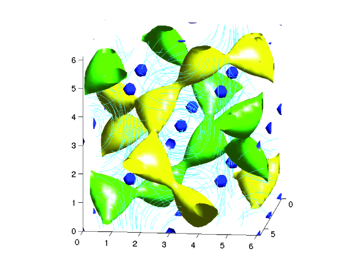
(a)

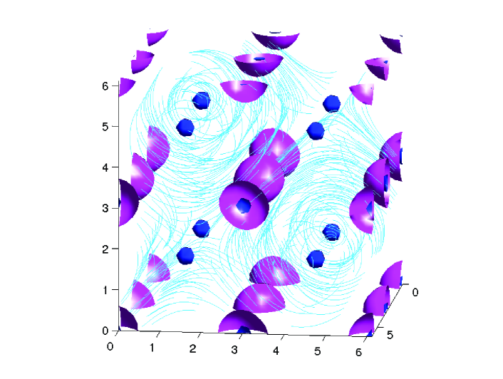
(b)

Figure 2: Optimal at $\mbox{\it Rm}_{c}=1.737$ . (a) Isosurfaces of positive and negative helicity $\mbox{\boldmath$u$}\cdot{\mbox{\boldmath$\omega$}}$ (yellow, green) and stagnation points (blue). (b) Isosurfaces of $\mbox{\boldmath$B$}_{T}^{2}$ (pink). Blue lines in (a) and (b) are respectively streamlines and magnetic field lines.

Although the optimal can be traced a little beyond $\mbox{\it Rm}=2$, it becomes clear that its basin of optimality (with respect to $\mathcal{L}$) quickly becomes vanishingly small, as not all optimisations converge. When the optimisation converges, the velocity and magnetic field are well resolved, and the energy spectrum of the Fourier coefficients falls by 16 orders. But for only slightly larger Rm, other velocity fields that include highly localised regions of strain are also picked up by the optimisation, and large strain is known to lead to large growth Galanti92 . While the scaled velocity satisfies $||\mbox{\boldmath$u$}||_{2}=1$, the strain rate $S=(2\,S_{ij}\,S_{ij})^{1/2}$, where $S_{ij}=\frac{1}{2}(\partial_{i}\,u_{j}+\partial_{j}\,u_{i})$, is unlimited. Hence the growth is unlimited and the optimisation fails.

A more appropriate measure of the flow is therefore necessary, here taken to be the velocity scale $U=L\,||S||_{2}$. Whilst $S$ and the vorticity $|\mbox{\boldmath$\omega$}|$ are not equal locally, it can be shown that $||S||_{2}=||\mbox{\boldmath$\omega$}||_{2}$. The latter is somewhat more convenient to work with in the variational method. The scaled velocity field then satisfies $||\mbox{\boldmath$\omega$}||_{2}=1$, so that optimisation can be considered to be over the space of fields with equal viscous dissipation or input power driving the flow, neglecting any feedback on the flow from the magnetic field. This scaling leads to the magnetic Reynolds number

$$\mbox{\it Rm}_{\omega}=\frac{L^{2}\,||\mbox{\boldmath$\omega$}||_{2}}{\lambda}.$$ (10)

In a similar context, Backus Backus58 derived a lower limit for dynamos in a sphere in terms of the analogous magnetic Reynolds number except involving $||S||_{\infty}$ rather than $||S||_{2}$. Although not used further here, higher norms of $S$ and $\omega$ are observed to behave similarly.

The optimisation is only slightly altered, where now

$$\mathcal{L}=\langle\mbox{\boldmath$B$}_{T}^{2}\rangle\,-\,\lambda_{1}(\langle\mbox{\boldmath$\omega$}^{2}\rangle-1)\,-\,\dots$$ (11)

and the new update is given by

$$\frac{\delta\mathcal{L}}{\mbox{\boldmath$\delta u$}}~{}=\int_{0}^{T}\mbox{\boldmath$B$}\times(\mbox{\boldmath$\nabla$}\times\mbox{\boldmath$\Gamma$})\,\mathrm{d}t-2\lambda_{1}\,\mbox{\boldmath$\nabla$}\times\mbox{\boldmath$\omega$}+\mbox{\boldmath$\nabla$}\Pi_{1}.\\$$ (12)

Similar to before, the scalar $\lambda_{1}$ is chosen such that for the new $u$ one has $\langle\mbox{\boldmath$\omega$}^{2}\rangle=1$. The extra complexity of the update leads to a linear approximation that is valid over a shorter range, and the number of iterations necessary for convergence is typically order 1000, compared with order 100 before.

Upon optimisation with the vorticity scaling, zero growth rate is found at $\mbox{\it Rm}_{\omega c}=2.48$. The optimal velocity field is structurally almost identical to that found previously at $\mbox{\it Rm}_{c}=1.737$, but for the new velocity field, its corresponding $\mbox{\it Rm}=1.75$, now an observed quantity, is slightly higher. Starting from 40 initial conditions at $\mbox{\it Rm}_{\omega c}$, all converged to the same optimal. Figure 3 compares growth rates for the optimal found at $\mbox{\it Rm}_{c}=1.737$, where $\mbox{\boldmath$u$}_{op}$ is fixed and $\mbox{\it Rm}_{\omega}$ is varied, with the optimal that could now be tracked up to $\mbox{\it Rm}_{\omega}=100$. For this range of $\mbox{\it Rm}_{\omega}$ the fixed velocity field is competitive with the optimised state, which changes relatively little. From $\mbox{\it Rm}_{\omega}=2.48$ to $100$ it remains an optimal with only a relative change of 8%. Although the inset shows that the optimal at $\mbox{\it Rm}_{\omega}=50$ remains fairly robust to perturbations, at these larger magnetic Reynolds numbers, other optimals are likely to exist.

Beyond $\mbox{\it Rm}_{\omega}=100$, convergence was found to be possible using a higher norm $||\mbox{\boldmath$\omega$}||_{4}$, but this incurs further iterations for convergence. Optimisation at higher Rm becomes computationally expensive — in addition to increased spatial resolution and more iterations, larger target times $T$ are necessary to pass longer transients.

\psfrag{E}{\small$\langle\mbox{\boldmath$B$}^{2}\rangle$}\psfrag{t}{\small$t$}\psfrag{s}{\small$\sigma$}\psfrag{d}{\small$d$}\psfrag{RmS}{\small$\mbox{\it Rm}_{\omega}$}\includegraphics[width=346.89731pt]{figs/3870Growth2}

Figure 3: Growth rates, $\sigma$ in units $||\mbox{\boldmath$\omega$}||_{2}$, for the optimal at $\mbox{\it Rm}_{c}=1.737$ (red, solid), where the velocity is held fixed. This is bounded above by the optimisation at each $\mbox{\it Rm}_{\omega}$ (blue, dashed); $\mbox{\it Rm}_{\omega c}=2.48$. Inset: Growth rates for perturbations to the optimal at $\mbox{\it Rm}_{\omega}=50$ with $||\mbox{\boldmath$\omega$}||=1$; disturbances defined similarly in Fig. 1.

Time dependence of the velocity field is an important factor that could affect magnetic energy growth. In order for energy growth to be enhanced, the changing velocity field must exploit transient energy growth to beat the mean of the energy growths associated with each velocity field considered separately. At low Rm, however, this affect has barely been observed. Setting $T$ to a small value permits calculation of velocity and magnetic fields that lead to the largest initial magnetic energy growth. Starting the optimisation from $40$ initial conditions and taking $T=0.05$, two optima were identified, shown in Fig. 4. The lowest $\mbox{\it Rm}_{\omega}$ for which the maximum initial growth was zero set the energy stability bound at $\mbox{\it Rm}_{\omega g}=2.12$. Between $\mbox{\it Rm}_{\omega g}$ and $\mbox{\it Rm}_{\omega c}$ it is possible to find brief growth of the magnetic field, but ultimately it decays.

\psfrag{E}{\small$\langle\mbox{\boldmath$B$}^{2}\rangle$}\psfrag{t}{\small$t$}\includegraphics[width=268.84227pt]{figs/3885Bt}

Figure 4: Development of energy following optimised initial growth; $Rm_{\omega g}=2.12$. The local optimal for which growth is initially zero defines $Rm_{\omega g}$ (red, solid), but rapid decay immediately follows the initial ‘burst’. A second optimal (blue, dashed) decays monotonically but more slowly. This second optimal is connected to that for a steady field at the slightly higher $\mbox{\it Rm}_{\omega c}=2.48$.

The small difference between $\mbox{\it Rm}_{\omega g}$ and $\mbox{\it Rm}_{\omega c}$ leaves little room for reduction of $\mbox{\it Rm}_{\omega c}$ gained by time-dependence of velocity fields. Transient growth will, however, be very important at large Rm.

In summary, a minimum magnetic Reynolds number is found for a kinematic dynamo at $\mbox{\it Rm}_{\omega c}=2.48$, by optimisation over the space of velocity fields with equal $||\mbox{\boldmath$\omega$}||_{2}$ or associated viscous dissipation. Starting from 40 random initial conditions at this $\mbox{\it Rm}_{\omega}$, all converged to the same optimal. This velocity field is very close to an optimal at $\mbox{\it Rm}_{c}=1.737$ in the space of fields with $||\mbox{\boldmath$u$}||_{2}=1$ . In the latter space, other fields with high strain-rate are also possible. The optimal velocity field appears to be a fast dynamo, with a growth rate $\sigma=0.358\,||\mbox{\boldmath$\omega$}||_{2}=0.529\,||\mbox{\boldmath$u$}||_{2}/L$, but optimisation at larger Rm is likely to lead to the identification of more efficient dynamos. A lower bound for instantaneous magnetic energy growth is found at $\mbox{\it Rm}_{\omega g}=2.12$, not far below $\mbox{\it Rm}_{\omega c}=2.48$.

As shown here, the variational method can be used to identify velocity fields that maximise magnetic energy growth, and to determine a lower bound on the critical Reynolds number for a dynamo. It is a rare occasion that we can put a numerical figure to such an important parameter. In geometries closer to experiments, tricky boundary conditions on the magnetic field for spheres and cylinders pose technical challenges, but it will be worthwhile overcoming them. It will be interesting to see if velocity fields realisable in experiment are close, or can be made closer, to optimal. That the growth rate is observed to change little for perturbations about the optimal, is promising for the dynamo’s robustness. It will also be of interest to further assess the mechanism that optimises growth, and future optimisations at higher Rm may identify alternative optimals and dynamo mechanisms to that observed here.

- (1) H. K. Moffatt, Magnetic field generation in electrically conducting fluids (Cambridge University Press, 1978)
- (2) A. D. Gilbert, Geophys. Astrophys. Fluid Dyn. 44, 241 (1988)
- (3) G. O. Roberts, Phil. Trans. R. Soc. Lond. A 266, 535 (1970)
- (4) V. I. Arnold, C. R. Acad. Sci. Paris 17, 261 (1965)
- (5) S. Childress, J. Math. Phys. 11, 3063 (1970)
- (6) M. Dudley and R. James, Proc. R. Soc. Lond. A 425, 407 (1989)
- (7) A. Alexakis, Phys. Rev. E 84, 026321 (2011)
- (8) A. Gailitis, O. Lielausis, E. Platacis, S. Dement’ev, A. Cifersons, G. Gerbeth, T. Gundrum, F. Stefani, M. Christen, and G. Will, Phys. Rev. Lett. 86, 3024 (2001)
- (9) R. Stieglitz and U. Müller, Phys. Fluids 13, 561 (2001)
- (10) R. Monchaux, M. Berhanu, M. Bourgoin, M. Moulin, P. Odier, J.-F. Pinton, R. Volk, S. Fauve, N. Mordant, F. Pétrélis, A. Chiffaudel, F. Daviaud, B. Dubrulle, C. Gasquet, L. Marié, and F. Ravelet, Phys. Rev. Lett. 98, 044502 (2007)
- (11) S. Zuccher, A. Bottaro, and P. Luchini, Eur. J. Mech. B, Fluids 25, 1 (2006)
- (12) C. C. T. Pringle and R. R. Kerswell, Phys. Rev. Lett. 105, 154502 (2010)
- (13) C. C. T. Pringle, A. P. Willis, and R. R. Kerswell, J. Fluid Mech. 702, 415 (2012)
- (14) V. Archontis, S. B. F. Dorch, and Å. Nordlund, Astron. Astrophys. 397, 393 (2003)
- (15) B. Galanti, P. Sulem, and A. Pouquet, Geophys. Astrophys. Fluid Dyn. 66, 183 (1992)
- (16) G. Backus, Ann. Phys. 4, 372 (1958)
- (17) For comparison, the space of ABC flows is possibly a restrictive space of flows, but at the same time it is sufficiently large to make the parameter search a substantial feat. Within this class it has nevertheless been possible to identify the Roberts flow as being optimal Alexakis11 . For this geometry (-wavenumber ) the critical magnetic Reynolds number for Roberts flow is . For the traditional ABC flow (), .