Characterization of Young Stellar Clusters

Abstract

Aims. A high number of embedded clusters is found in the Galaxy. Depending on the formation scenario, most of them can evolve to unbounded groups that are dissolved within a few tens of Myr. A systematic study of young stellar clusters showing distinct characteristics provide interesting information on the evolutionary phases during the pre-main sequence. In order to identify and to understand these phases we performed a comparative study of 21 young stellar clusters.

Methods. Near-infrared data from 2MASS were used to determine the structural and fundamental parameters based on surface stellar density maps, radial density profile, and colour-magnitude diagrams. The cluster members were selected according to the membership probability, which is based on the statistical comparison with the cluster proper motion. Additional members were selected on basis of a decontamination procedure that was adopted to distinguish field-stars found in the direction of the cluster area.

Results. We obtained age and mass distributions by comparing pre-main sequence models with the position of cluster members in the colour-magnitude diagram. The mean age of our sample is $\sim$ 5 Myr, where 57% of the objects is found in the 4 - 10 Myr range of age, while 43% is $<$ 4 Myr old. Their low E(B-V) indicate that the members are not suffering high extinction ($A_{V}<1$ mag), which means they are more likely young stellar groups than embedded clusters. Relations between structural and fundamental parameters were used to verify differences and similarities that could be found among the clusters. The parameters of most of the objects have the same trends or correlations. Comparisons with other young clusters show similar relations among mass, radius and density. Our sample tends to have larger radius and lower volumetric density, when compared to embedded clusters. These differences are compatible with the mean age of our sample, which we consider intermediary between the embedded and the exposed phases of the stellar clusters evolution.

1 Introduction

It is generally known that most stars are formed in groups or clusters. However, detailed studies on the initial processes of star formation are restricted to isolated dense cores of clouds (Shu et al. (1987); Shu 2004 (2004)).

The first stages of multiple star formation is usually evaluated through millimetric surveys, which are successful probing the scenario of stellar clusters formation. Based on 1.2mm data of the Mon OB1 region, for instance, Peretto et al. (2005) discovered 27 proto-stellar cores with diameters of about 0.04 pc and masses ranging from 20 to 40 M_⊙ associated to the young stellar cluster NGC 2264. These results reveal the physical conditions for multiple massive star formation in a region that shows a wide range of masses (Dahm (2008)) and ages (Flaccomio et al. (1997); Rebull et al. (2002)) indicating the occurrence of a large variety of young stellar groups.

In addition to millimetric studies, the evolution during the pre-main sequence (pre-MS) is more closely surveyed by using infrared data. Particularly, near-infrared (NIR) provides information about the circumstellar structure of the cluster members, whose physical conditions are directly related to the pre-MS evolutionary stage of the star. Gregorio-Hetem et al. (2009), for instance, have used X-ray results of sources detected in CMa R1, combined with NIR and optical data, to identify the young population associated to this star-forming region. They studied two young clusters having similar mass function, but one of them is older than the other by at least a few Myr. A mixing of populations seems to occur in the inter-clusters region, possibly related to sequential star formation.

Systematic studies of young stellar clusters can directly probe several fundamental astrophysical problems, such as formation and evolution of open clusters, and more general problems, like the origin and early evolution of stars and planetary systems (Adams et al. 2006, Adams (2010)).

Kharchenko et al. (2005) presented angular sizes of cluster core and “coronae” for a sample of 520 Galactic open clusters, and Piskunov et al. (2007) revised these data to obtain tidal radius and core size estimated by fitting King profile to the observed density distribution.

Carpenter (2000) used 2MASS data to derive surface density maps of stellar clusters associated to molecular clouds, determining cluster radius and number of members based on the distributed population.

Adams et al. (2006) explored the relations between cluster radius and stellar distribution in order to study the dynamical evolution of young clusters. Numerical simulations were used to reproduce different initial conditions of cluster-formation. The statistical calculations developed by Adams et al. (2006) were based on cluster membership and cluster radius correlations observed in the samples presented by Carpenter (2000) and Lada & Lada (2003), who compiled the first extensive catalogue of embedded clusters providing parameters such as mass, radius and number of members.

Lada & Lada (2003), hereafter LL (03), verified the occurrence of a high number of embedded clusters within molecular clouds in the Galaxy. However, most of these objects probably lose their dynamical equilibrium that would dissolve the group turning it into field-stars.

Pfalzner 2009 (2009) studied the evolution of a sample of 23 massive clusters younger than 20 Myr, suggesting two distinct sequences. Depending on size and density, a bimodal distribution is found for the cluster size as a function of age. Based on the mass-radius and density-radius dependence observed in the sample from LL (03), Pfalzner (Pfalzner 2011 (2011)) proposed a scenario of sequential formation of “leaky” (exposed) massive clusters.

On the other hand, differently of the time sequence proposed by Pfalzner (Pfalzner 2011 (2011)), the relations of cluster properties can be interpreted as formation condition (Adams et al. 2006, Adams (2010)).

The structure of embedded clusters traces the physical conditions of their star-forming processes, since the origin and the evolution of stellar clusters are related to the distribution of dense molecular gas in their parental cloud. LL (03) proposed two basic structural types, according to the cluster surface density. Classical open clusters are characterised by a high concentration in their surface distribution, whose radial profile is smooth and can be reproduced by simple power law functions or King-like (isothermal) potential. This type of embedded cluster is considered centrally concentrated. On the other hand, hierarchical type clusters exhibit surface density distribution with multiple peaks and show significant structure over a large range of spatial scale. Although there are clear examples of both types of structures, their relative frequency is unknown.

The main goal of the present work is to characterise a large sample of young stellar clusters and to perform a comparative study aiming to verify their similarities and differences, which are related to their evolutionary stages in the pre-MS.

The methods adopted by us have been commonly used in the characterization of open clusters like those developed by Bonatto & Bica (2009a), for instance. Stellar density maps are built from NIR data in order to derive parameters on the basis of radial density profile. These parameters define the structure of the cluster, which is related to its origin and evolution.

The analysis based on radial density profile is unprecedented to 86% of our sample. Considering the lack of systematic studies comparing pre-MS stellar clusters, distributed in different galactic regions, the present work aims to provide sets of structural and fundamental parameters, determined in a uniform data analysis that may contribute to the discussion on the origin of stellar groups.

In Sect. 2 we describe the sample by presenting the selection criteria and the decontamination method for distinguishing cluster members from field-stars. Section 3 is dedicated to determine the structural parameters, which are used to accurately determine distance, age and mass that are presented in Sect. 4. A comparative analysis is performed in Sect. 5, while Sect. 6 summarises the results and the main conclusions. Finally, Appendix A displays all the plots of the entire sample.

Table 1: List of clusters and their structural parameters.

Cluster	$\alpha$	$\delta$	R	$\sigma_{bg}$	$\sigma_{0}$	$<n_{*}>$	rc	$\delta_{c}$	rc/R	Class
	(h m s)	(o ’)	(pc)	(pc-2)	(pc-2)	(pc-2)	(pc)
Collinder 205	09 00 31(5)	-48 59	3.4$\pm$1.2	9$\pm$3	51$\pm$16	4.8$\pm$1.9	0.30$\pm$0.03	6.6$\pm$2.6	0.09$\pm$0.03	??
Hogg 10	11 10 40(9)	-60 14	1.9$\pm$0.4	16$\pm$2	9$\pm$4	7.6$\pm$1.7	0.46$\pm$0.28	1.6$\pm$0.3	0.24$\pm$0.15	H
Hogg 22	16 46 35(6)	-47 05	1.9$\pm$0.5	20$\pm$4	7$\pm$3	9.0$\pm$3.8	1.91$\pm$1.10	1.3$\pm$0.2	1.03$\pm$0.65	H
Lynga 14	16 55 03(5)	-45 14	1.1$\pm$0.4	55$\pm$18	153$\pm$52	16.7$\pm$7.0	0.22$\pm$0.04	3.8$\pm$1.3	0.20$\pm$0.08	CC
Markarian 38	18 15 15(5)	-19 01	1.6$\pm$0.5	18$\pm$6	44$\pm$15	6.8$\pm$2.3	0.13$\pm$0.03	3.4$\pm$1.2	0.08$\pm$0.03	CC
NGC 2302	06 51 55(4)	-07 05	2.3$\pm$0.5	8$\pm$2	16$\pm$4	4.0$\pm$1.4	0.54$\pm$0.10	3.0$\pm$0.6	0.23$\pm$0.06	CC
NGC 2362a	07 18 42(4)	-24 28	1.9$\pm$0.4	13$\pm$3	62$\pm$14	3.3$\pm$1.0	0.26$\pm$0.05	5.8$\pm$1.7	0.13$\pm$0.04	CC
NGC 2367	07 20 06(4)	-21 53	2.9$\pm$0.7	5$\pm$1	13$\pm$3	2.3$\pm$0.6	0.34$\pm$0.11	3.6$\pm$0.7	0.12$\pm$0.05	??
NGC 2645	08 39 05(6)	-46 14	2.1$\pm$0.5	13$\pm$3	48$\pm$12	7.5$\pm$2.1	0.22$\pm$0.04	4.8$\pm$1.2	0.10$\pm$0.03	??
NGC 2659	08 42 37(6)	-44 59	3.6$\pm$0.5	9$\pm$1	11$\pm$2	5.2$\pm$0.9	1.93$\pm$0.37	2.2$\pm$0.3	0.53$\pm$0.12	H
NGC 3572	11 10 26(8)	-60 15	2.5$\pm$0.5	19$\pm$3	76$\pm$15	7.7$\pm$1.9	0.16$\pm$0.03	5.0$\pm$1.1	0.06$\pm$0.02	H
NGC 3590	11 12 59(7)	-60 47	1.5$\pm$0.4	30$\pm$7	96$\pm$27	11.7$\pm$4.5	0.29$\pm$0.06	4.2$\pm$1.2	0.20$\pm$0.07	CC
NGC 5606	14 27 48(8)	-59 38	2.6$\pm$0.4	11$\pm$2	25$\pm$5	4.8$\pm$0.9	0.51$\pm$0.13	3.2$\pm$0.6	0.20$\pm$0.06	CC
NGC 6178	16 35 47(6)	-45 39	1.7$\pm$0.4	24$\pm$4	32$\pm$11	12.2$\pm$2.7	0.30$\pm$0.12	2.3$\pm$0.5	0.18$\pm$0.08	H
NGC 6604b	18 18 04(3)	-12 15	2.6$\pm$0.7	11$\pm$3	17$\pm$5	4.4$\pm$1.3	0.50$\pm$0.11	2.6$\pm$0.6	0.19$\pm$0.07	H
NGC 6613	18 19 58(4)	-17 06	2.9$\pm$0.7	9$\pm$2	82$\pm$19	4.9$\pm$1.2	0.12$\pm$0.01	10.6$\pm$3.5	0.04$\pm$0.01	CC
Ruprecht 79	09 40 59(7)	-53 51	3.9$\pm$0.5	7$\pm$1	4$\pm$1	3.6$\pm$0.5	2.2$\pm$0.8	1.5$\pm$0.2	0.57$\pm$0.22	CC
Stock 13c	11 13 04(8)	-58 53	2.3$\pm$0.3	15$\pm$2	42$\pm$14	3.8$\pm$0.9	0.11$\pm$0.05	3.8$\pm$1.0	0.05$\pm$0.02	H
Stock 16	13 19 30(8)	-62 38	2.8$\pm$0.7	15$\pm$3	8$\pm$4	5.8$\pm$1.6	1.2$\pm$0.6	1.5$\pm$0.3	0.42$\pm$0.24	H
Trumpler 18	11 11 27(9)	-60 40	4.6$\pm$0.8	9$\pm$1	15$\pm$4	2.5$\pm$0.4	0.38$\pm$0.10	2.8$\pm$0.5	0.08$\pm$0.03	H
Trumpler 28	17 37 02(5)	-32 38	1.4$\pm$0.5	9$\pm$4	25$\pm$9	12.3$\pm$4.5	0.84$\pm$0.16	3.7$\pm$1.4	0.61$\pm$0.24	H

Columns description: (1) Identification; (2, 3) J₂₀₀₀ coordinates; (4) cluster radius; (5) background density; (6) core density; (7) observed average density; (8) core radius; (9) density-contrast parameter; (10) ratio of core-size to cluster-radius; (11) cluster type: hierarchical (H), centrally concentrated (CC), undefined (??). Notes: parameters from Piskunov et al. : (a) $R_{c}$=0.6$\pm$0.4 pc; (b) $R_{c}$= 2.4$\pm$1.4pc; (c) $R_{c}$=1.0$\pm$0.8 pc.

2 Description of the sample

Several compilations of open stellar clusters are available in the literature, for example Lynga (1987), Loktin (1994), Mermilliod (1995), LL (03), Kharchenko et al. (2005), Piskunov et al. , WEBDA and DAML (Dias et al. (2002); Dias 2006 (2006)), among others. In Sect. 2.1 we present the criteria used to select the clusters, while Sect. 2.2 describes the method used to exclude field-stars that were found in the same direction of the cluster.

2.1 Clusters selection and observational data

Aiming to focus our study on pre-MS objects, the DAML catalogue was used to select young stellar clusters with ages in the 1 - 20 Myr range. Distances smaller than 2 Kpc were used as selection criterion in order to ensure good quality of photometric data. Despite our selection is limited to southern objects, they are distributed in different star-forming regions enabling us to compare diverse environments. Table 1 gives the list of 21 selected clusters.

A membership probability (P) estimated on basis of proper motion is given by DAML. For the selection of stars belonging to the clusters, the values P$>$ 50% were adopted to indicate the possible members, hereafter denoted by P50.

In order to confirm the cluster centre coordinates available in the literature, we evaluated the distribution of number of stars as a function of right ascension ($\alpha$) and declination ($\delta$). Gaussian profiles were fitted to these distributions, in order to estimate their centroid. A good agreement with the literature was found, within the errors estimated by the fitting that are $\Delta\delta\sim$ 1 arcmin and 0.75’$<\Delta\alpha<$ 2.25’. Table 1 gives the error on $\alpha$ indicated in between parenthesis.

The NIR data, which provide maximum variation among colour-magnitude diagrams (CMDs) of clusters with different ages (Bonatto, Bica & Girardi (2004)), were extracted from 2MASS (All Sky Catalogue of Point Sources - Cutri et al. (2003)). The JHK_s magnitudes were searched for all stars located within a radius of 30 arcmin from the cluster centre. Only good accuracy photometric data were used in our analysis, by selecting objects with AAA quality flags that ensure the best photometric and astrometric qualities (Lee et al. (2005)).

2.2 Field-stars decontamination

Most of our clusters are projected against dense fields of stars in the Galactic disk, making difficult to distinguish the cluster members. The first step to determine the structural and fundamental parameters is to proceed the field-stars decontamination.

This process is based on statistical analysis by comparing the stellar density of the cluster area with a reference region, near to the cluster, according to their characteristics in the CMD. The decontamination algorithm was employed as follows:

• the whole range of magnitudes and colours is divided into three dimensional cells (J, J-H and J-K_S);

• for each cell ($i$), the stellar density of field-stars ($\sigma_{f}$ = n_f / a_f) is obtained by counting the number of stars (n_f) appearing in the reference region (a_f);

• similarly, the total stellar density ($\sigma_{t}$ = n_t / a_c) is obtained by counting all stars (n_t) in the cluster area (a_c);

• the number of field-stars ($n_{f}$), appearing in the cluster area, that have colours and magnitude similar to those estimated in the reference region is calculate by:

  $$n_{f}=\frac{\sigma_{f}}{\sigma{t}}\times n_{t}$$ (1)

• Finally, the number of field-stars in the cluster area is randomly subtracted in each cell, remaining $N=\Sigma_{i}\ (n_{t_{i}}-n_{f_{i}}$) members of the cluster.

In order to minimize errors introduced by the parameters choice and uncertainties on 2MASS data, the decontamination algorithm is applied to several grids by adopting three different positions in the CMD. By defining a cell size $\Delta J$ = 0.5 mag, the algorithm uses a grid starting at $J_{i}$ and two other grids starting at $J_{i}\pm\frac{1}{3}\Delta J$. This dithering is also made for both colours, $\Delta$(J-H) = $\Delta$(J- K_S) = 0.1 mag, providing 27 different results for each star. By this way, we obtain the probability that a given object should be considered a field-star. All possible members (P50) have 0% of probability of being a field-star.

We considered as candidate members (denoted by P?) the stars that were not removed by the field-star decontamination. Both, P50 and P? members were used, but having different weight, in the estimation of distance and age, presented in Sect. 4.2.

The adopted decontamination procedure has been used in studies of several types of clusters: objects showing low contrast relative to the field-stars (Bica & Bonatto (2005), embedded clusters (Bonatto, Santos Jr. & Bica (2006)), young clusters (Bonatto et al. (2006)), among others.

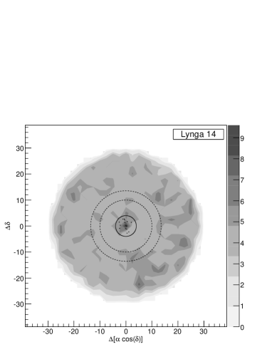
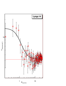
Figure 1: Left: Stellar surface-density map ($\sigma$ (stars/arcmin²)) obtained for the region of 30 arcmin around Lynga 14. The comparison field-stars area is indicated by dashed lines, while the full line indicates the cluster area. Center: a zoom of the $\sigma$ map indicating by crosses the position of objects with membership probability P$>$70%. Right: The distribution of the stellar density as a function of radius. The best fitting of observed radial density profile, indicated by the full line, was obtained by using the model from King (1962). A red line indicates the background density ($\sigma_{bg}$).

3 Structural parameters

The structural parameters were determined on basis of stellar surface density, derived from stellar surface-density maps and radial density profile that are detailed in the Sects. 3.1 and 3.2.

The first step, in the calculation of the stellar surface density, is to enhance the contrast between surface distribution of cluster members and field-stars by using a colour-magnitude filter.

Pre-MS isochrones were adopted to establish the colour-magnitude filter limiting a CMD region that should contain only cluster members. Once the observed magnitudes were unreddened, using the visual extinction given in the literature, we disregarded all the objects lying out of the range defined by the colour-magnitude filter. This filter is successful to accentuate the structures and to reduce the fluctuations caused by the presence of field-stars (Bica & Bonatto (2005)).

3.1 Stellar surface-density maps

We obtained spatial distribution maps of the stellar surface density ($\sigma$) given by the number of stars per arcmin² for the clusters and their surroundings. Appendix A presents the results for the whole sample, while Fig. 1 shows the map derived for the cluster Lynga 14, as illustration. The left panel shows the entire studied area, whose surface density was calculated in cells of $|\Delta(\alpha cos(\delta_{center}))|=|\Delta\delta|$ = 2.5 arcmin², where $\Delta\alpha$ and $\Delta\delta$ are the steps on right ascension and declination, respectively. The dashed annulus corresponds to the reference field-stars region and the central circle indicates the cluster area.

A zoom view (Fig. 1 central panel) displays a more detailed structure that was obtained by using smaller cells (1.0 arcmin²) for the star counting process. Following the classification proposed by LL (03), the surface density maps were visually inspected to characterise the clusters. Last column of Table 1 indicates if the type is Hierarchical (H) or Centrally Concentrated (CC), according to the definition discussed in Sect. 1. About 38% of the sample (8/21) shows a single major peak of density being classified by CC. Half of the sample (10/21) has multiple peaks and were considered of H type, while three objects presenting filamentary density distributions, have undefined type (marked as “??” in Table 1).

3.2 Radial density profile

Aiming to quantify the stellar distribution of the clusters, we evaluated their radial density profile (RDP) by using concentric rings to calculate the surface density.

Some of the structural parameters were obtained by fitting a theoretical RDP to the observed data. The adopted function is similar to the empirical model from King (1962), given by:

$$\sigma(r)=\sigma_{bg}+\frac{\sigma_{0}}{1+(r/r_{c})^{2}}$$ (2)

where $\sigma(r)$ is the stellar surface density (stars/arcmin²), r is the radius (arcmin) of each concentric annulus used in the star counting, $\sigma_{0}$ and $r_{c}$ are respectively the density and the radius of the cluster core. The average density measured in the reference region ($\sigma_{bg}$) was calculate separately, in order to diminish the number of free parameters in the RDP fitting.

Figure 1 (right panel) shows an example of observed radial distribution of surface density and the best fitting of the King’s profile, which was obtained by adopting the $\chi^{2}$ method based on the parameters $\sigma_{0}$ and $r_{c}$.

Aiming to determine the cluster radius (R) more accurately, we verified the point where the cluster stellar density reaches the background density. Figure 1 displays a red line corresponding to $\sigma=\sigma_{bg}$ that was used to find R.

A quantitative estimation on how compact is the cluster can be obtained from the density-contrast parameter proposed by Bonatto & Bica (2009a):

$$\delta_{c}=1+\frac{\sigma_{0}}{\sigma_{bg}}$$ (3)

where compact clusters have $7\ \leq\ \delta_{c}\ \leq 23$. According this this criterion, only NGC 6613 can be considered compact ($\delta_{c}\sim$ 10).

Two other parameters are usual in comparative analysis: the average density ($<n_{*}>$), calculated by dividing the total number of observed members by the cluster area, and the ratio of core-size to cluster-radius (r_c/R). We could expect small values of r_c/R for the younger clusters, since their members would not have had enough time to disperse away from the centre.

Table 1 gives the structural parameters and the uncertainties derived from the RDP fitting.

Three of our objects are found in the catalogue of Galactic open clusters presented by Piskunov et al. . Based on proper movement, they identified bright stars( V $<$ 14 mag) and used the radial profile of the region containing possible members (P=14-61%) to define the “coronae” radius of the cluster, while the concentration of the probable members (P$>$61%) defines the core radius (Kharchenko et al. 2005). Therefore, their sample is 5 to 10 times less numerous than our sample that includes low-mass stars detected by 2MASS. Besides, we focused on the main stellar distribution of the cluster (radius $<6^{\prime}$), while they studied larger areas (radius $\sim 15^{\prime}$), seeking for the tidal radius ($R_{t}$).

These different definitions of cluster radii, imply in systematically smaller values when comparing our results with the structural parameters listed by them. However, these results cannot be directly compared because we are not dealing with the same kind of stellar groups.

In fact, the tidal radius obtained by Piskunov et al. (2007) for NGC 6604 ($R_{t}$=8.8pc); NGC 2362 (6.2pc); and Stock 13 (7pc) is more compatible with the tidal radius that we estimated for these clusters: $r_{t}$= 7.7$\pm$2.3; 8.1$\pm$2.4; and 7.0$\pm$2.1, respectively, by adopting the expression used by Saurin, Bica & Bonatto (SBB2012 (2012)):

$$r_{t}=(\frac{M}{M_{gal}})^{1/3}d_{GC}$$ (4)

where M is the cluster mass, M_gal is the Galactic mass and d_GC is the Galactocentric distance, given by:

$$M_{gal}=\frac{V^{2}_{GC}d_{GC}}{G}$$ (5)

where V_GC = 254$\pm$16 km/s is the circular rotation velocity of the Sun at R_GC = 8.4$\pm$0.6 kpc (Reid et al. (2009)).

On the other hand, the R $\propto$ N^0.5 dependence discussed in Sect. 5.1 distinguishes the sample studied by Piskunov et al. (2007) from other young clusters presenting size and membership relations similar to our sample. It seems to be more consistent comparing the cluster radius that we obtained with the core radius obtained by Piskunov et al. , given as notes in Table 1.

4 Revisiting the fundamental parameters

Adopting the same procedure described in Sect. 2.2, the field-stars decontamination was refined by using the accurate estimative of cluster radius. The size of the reference region was also re-evaluated according to the cluster area, allowing us to more closely define the sample of candidate members.

In Sect. 4.1 we adopt the extinction available in the literature to correct the observed colours, which were fitted to the MS intrinsic colours. An iterative fitting process was adopted to accurately determine E(B-V).

Despite the distance and age of our clusters are available in the literature, these parameters were checked by us on the light of the well determined structural parameters, as described in Sect. 4.2.

4.1 Colour excess

The (J-H) and (H-K_s) colours were used to estimate the extinction, by evaluating the position of the cluster members compared to the MS. In Fig. 2 (left panel), we plot the intrinsic colours of MS and giant stars given by Bessel and Brett (1988), as well as the corresponding reddening vectors given by Rieke and Lebofsky (1985). For comparison, the Zero Age Main-Sequence (ZAMS) from Siess et al. (2000) is also plotted, which has quite the same distribution of the MS, mainly for massive stars.

Adopting the normal extinction law $A_{V}=3.09E(B-V)$ from Savage & Mathis (1979) and the relation $\frac{A_{\lambda}}{A_{V}}$ from Cardelli et al. (1989), the observed colours of the cluster members were unreddened and fitted to the MS intrinsic colours. This fitting is based on massive stars, mainly P50 members. Table 2 gives the E(B-V) that provides the best fitting, which is in good agreement with those available in the literature, within the estimated errors. Only a few objects had E(B-V) incompatible with the literature. In these cases, the procedure described in Sect. 3 for field-stars decontamination by using colour-magnitude filter was reapplied with the extinction derived by us, and the structural parameters were determined for this refined sample of cluster members.

The (J-H)_o and (H-K_s)_o colours were also used to reveal the stars with K-band excess. Young clusters are expected to have a large number of members showing high E(H-K_s) (Lada et al. (1996)). These stars appear in the right side of the MS reddening vector in the colour-colour diagram (Fig. 2). The fraction f_K was calculated by dividing the number of stars having large (H-K_s)_o by the total number of cluster members.

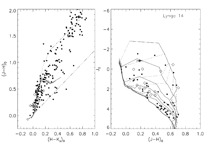
Figure 2: Left: Colour-colour diagram for Lynga  14. The MS and the ZAMS are indicated by full lines, while the locus of giant stars is represented by a dotted line. Reddening vectors from Rieke and Lebofsky (1985) are shown by dot-dashed lines. Right: Colour-magnitude diagram showing the isochrones and evolutionary pre-MS tracks from Siess et al. (2000). Cluster members are indicated by open diamonds (P50) and dots (P?).

4.2 Evaluation of distance and age

The unredenned magnitude and colour J_o $\times$ (J-H)_o of the cluster members were compared to pre-MS models (Siess et al. 2000) and also MS Padova models (Girard et al. (2002)) that were required to fit the colours of massive stars.

Figure 2 (right panel) shows the CMD obtained for Lynga 14, for illustration. The distances were confirmed by searching for $(m-M)_{Jo}$ that best fits the position of massive stars. The error bars were estimated from the minimum and the maximum distance module that provide good MS fittings. Within the uncertainties, the distances estimated from the MS fitting are in good agreement with the literature (differences are lower than 30%), excepting for Trumpler 18. Our results are presented in Table 2 and were used to convert into parsec the angular measurements of the structural parameters.

The number of stars as a function of age was obtained by counting the objects in between different pairs of isochrones in the CMD. We use bins of 5Myr, excepting the two first that correspond to 0.2 - 1 Myr and 1 - 5 Myr ranges. For MS objects (above the 7 M_⊙ track) we adopted the age estimated by fitting the data with Padova model. Figure 3 (left panel) shows the histogram of age distribution as a function of fractional number of members, where possible members (P50) and candidate members (P?) are displayed separately. Figures A3 to A7 show the plots used to evaluate age and mass for the whole sample.

The determination of age on basis of these histograms may not be obvious. Some of the clusters have members separated in two different ranges, making difficult the choice between the two options. The first choice of age is based on the most prominent peak formed by the P50 members. If the second peak has a similar number of members, we adopt the smaller value of age that is listed in Table 2, while the second option is given as notes in the same table.

Due to the large uncertainties on the age estimation, our conclusions are based on mean values. Considering that 12/21 objects of the sample (57%) are in the range of 4 - 10 Myr, and 9/21 (43%) are younger than 4 Myr, we suggest for our clusters a mean age of $\sim$ 5 Myr.

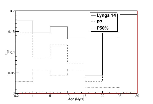
Figure 3: Left: Age distribution of Lynga 14 members (thick line) showing the contribution of P50 (dotted line) and P? (dashed line) objects. Right: Observed mass distribution indicated by crosses with error bars. The thick line represents the mass function $\phi$(m) fitting.

Table 2: Fundamental parameters.

Cluster	Age	E(B-V)	d	(m-M)	fk	Mobs	Nobs	MT	NT	$\chi$
	Myrs	mag	(pc)	mag	(%)	M⊙	(stars)	M⊙	(stars)
Collinder 205	5.0${}^{+5.0}_{-4.5}$	0.56$\pm$0.07	1800${}^{+500}_{-500}$	11.3${}^{+0.5}_{-0.7}$	14${}^{+17}_{-10}$	390 $\pm$ 79	174 $\pm$ 38	876 $\pm$ 262	2617 $\pm$ 701	1.17$\pm$0.33
Hogg 10	3.0${}^{+2.0}_{-2.0}$	0.23$\pm$0.05	2200${}^{+700}_{-400}$	11.7${}^{+0.6}_{-0.4}$	22${}^{+18}_{-15}$	218 $\pm$ 43	88 $\pm$ 10	318 $\pm$ 81	465 $\pm$ 149	0.59$\pm$0.17
Hogg 22a	3.0${}^{+2.0}_{-2.0}$	0.43$\pm$0.07	1700${}^{+550}_{-250}$	11.2${}^{+0.6}_{-0.3}$	28${}^{+19}_{-20}$	285 $\pm$ 47	97 $\pm$ 33	376 $\pm$ 99	429 $\pm$ 220	0.54$\pm$0.25
Lynga 14b	3.0${}^{+2.0}_{-2.5}$	0.50$\pm$0.10	950${}^{+200}_{-200}$	9.9${}^{+0.4}_{-0.5}$	6${}^{+16}_{-3}$	127 $\pm$ 30	68 $\pm$ 16	374 $\pm$ 111	1374 $\pm$ 430	1.24$\pm$0.21
Markarian 38	5.5${}^{+4.5}_{-4.5}$	0.10$\pm$0.07	1500${}^{+200}_{-250}$	10.9${}^{+0.3}_{-0.4}$	21${}^{+11}_{-12}$	137 $\pm$ 28	57 $\pm$ 3	190 $\pm$ 57	251 $\pm$ 107	0.52$\pm$0.27
NGC 2302c	2.5${}^{+2.5}_{-2.0}$	0.19$\pm$0.05	1700${}^{+300}_{-400}$	11.2${}^{+0.3}_{-0.6}$	26${}^{+19}_{-11}$	168 $\pm$ 32	70 $\pm$ 19	238 $\pm$ 57	345 $\pm$ 111	0.60$\pm$0.19
NGC 2362	4.0${}^{+6.0}_{-3.0}$	0.06$\pm$0.05	1480${}^{+400}_{-200}$	10.9${}^{+0.5}_{-0.3}$	31${}^{+17}_{-13}$	332 $\pm$ 55	124 $\pm$ 25	500 $\pm$ 126	927 $\pm$ 331	0.92$\pm$0.25
NGC 2367	3.0${}^{+2.5}_{-2.5}$	0.15$\pm$0.05	2200${}^{+400}_{-200}$	11.7${}^{+0.4}_{-0.2}$	20${}^{+12}_{-15}$	155 $\pm$ 29	60 $\pm$ 6	267 $\pm$ 64	586 $\pm$ 167	1.03$\pm$0.21
NGC 2645d	5.0${}^{+5.0}_{-4.0}$	0.28$\pm$0.08	1800${}^{+800}_{-200}$	11.3${}^{+0.8}_{-0.3}$	27${}^{+22}_{-18}$	238 $\pm$ 49	104 $\pm$ 14	498 $\pm$ 102	1366 $\pm$ 265	1.10$\pm$0.20
NGC 2659	5.0${}^{+10}_{-4.5}$	0.25$\pm$0.05	2000${}^{+500}_{-200}$	11.5${}^{+0.5}_{-0.2}$	28${}^{+21}_{-22}$	495 $\pm$ 103	215 $\pm$ 27	857 $\pm$ 237	1801 $\pm$ 608	0.89$\pm$0.22
NGC 3572	3.0${}^{+7.0}_{-2.5}$	0.15$\pm$0.07	1900${}^{+400}_{-200}$	11.4${}^{+0.4}_{-0.2}$	28${}^{+15}_{-16}$	371 $\pm$ 72	149 $\pm$ 22	645 $\pm$ 175	1422 $\pm$ 485	0.97$\pm$0.26
NGC 3590	2.5${}^{+1.5}_{-2.5}$	0.35$\pm$0.07	1680${}^{+500}_{-300}$	11.1${}^{+0.6}_{-0.4}$	34${}^{+23}_{-27}$	175 $\pm$ 36	79 $\pm$ 20	328 $\pm$ 90	768 $\pm$ 264	0.95$\pm$0.27
NGC 5606e	2.5${}^{+2.5}_{-2.3}$	0.32$\pm$0.05	2200${}^{+300}_{-200}$	11.7${}^{+0.3}_{-0.2}$	16${}^{+14}_{-9}$	262 $\pm$ 49	98 $\pm$ 11	417 $\pm$ 81	768 $\pm$ 147	0.86$\pm$0.13
NGC 6178f	5.0${}^{+2.5}_{-2.5}$	0.15$\pm$0.08	1430${}^{+150}_{-150}$	10.7${}^{+0.3}_{-0.2}$	6${}^{+9}_{-5}$	220 $\pm$ 52	106 $\pm$ 7	379 $\pm$ 284	1430 $\pm$ 1345	1.43$\pm$1.38
NGC 6604	6.0${}^{+4.0}_{-5.0}$	0.67$\pm$0.07	1600${}^{+400}_{-300}$	11.0${}^{+0.5}_{-0.4}$	18${}^{+16}_{-11}$	279 $\pm$ 52	90 $\pm$ 7	326 $\pm$ 95	245 $\pm$ 141	0.26$\pm$0.21
NGC 6613	5.0${}^{+5.0}_{-4.0}$	0.45$\pm$0.07	1550${}^{+300}_{-250}$	11.0${}^{+0.4}_{-0.4}$	26${}^{+15}_{-18}$	345 $\pm$ 73	133 $\pm$ 9	557 $\pm$ 113	1087 $\pm$ 185	0.93$\pm$0.13
Ruprecht 79	5.0${}^{+10}_{-4.5}$	0.28$\pm$0.05	2700${}^{+400}_{-300}$	12.2${}^{+0.3}_{-0.3}$	40${}^{+20}_{-25}$	459 $\pm$ 86	174 $\pm$ 8	677 $\pm$ 119	1156 $\pm$ 154	0.95$\pm$0.14
Stock 13	4.0${}^{+6.0}_{-3.0}$	0.07$\pm$0.05	2000${}^{+500}_{-350}$	11.5${}^{+0.5}_{-0.4}$	32${}^{+18}_{-15}$	179 $\pm$ 31	65 $\pm$ 11	308 $\pm$ 80	686 $\pm$ 236	1.02$\pm$0.26
Stock 16	7.0${}^{+8.0}_{-6.5}$	0.28$\pm$0.05	2000${}^{+500}_{-350}$	11.5${}^{+0.5}_{-0.4}$	30${}^{+19}_{-23}$	254 $\pm$ 66	139 $\pm$ 13	1043 $\pm$ 239	4676 $\pm$ 995	1.50$\pm$0.18
Trumpler 18	5.0${}^{+5.0}_{-4.0}$	0.10$\pm$0.07	2850${}^{+400}_{-350}$	12.3${}^{+0.3}_{-0.4}$	26${}^{+15}_{-14}$	512 $\pm$ 85	164 $\pm$ 8	572 $\pm$ 214	334 $\pm$ 543	0.00$\pm$0.17
Trumpler 28	2.0${}^{+3.0}_{-1.5}$	0.65$\pm$0.05	1050${}^{+250}_{-200}$	10.1${}^{+0.5}_{-0.5}$	10${}^{+25}_{-6}$	178 $\pm$ 35	73 $\pm$ 7	233 $\pm$ 58	268 $\pm$ 86	0.42$\pm$0.16

Columns description: (1) Identification; (2) age; (3)colour excess; (4) Distance; (5) distance modulus; (6) fraction of stars showing K excess; (7, 8) observed mass and number of members; (9, 10) total mass and number of members; (11) mass function slope.
Notes: Clusters showing a second peak on age distribution: (a) 12.5${}^{+2.5}_{-2.5}$; (b) 12.0${}^{+3.0}_{-7.0}$; (c) 12.5${}^{+2.5}_{-2.5}$; (d) 12.0${}^{+3.0}_{-7.0}$; (e) 11.5${}^{+3.5}_{-6.5}$; (f) 12.5${}^{+2.5}_{-2.5}$.

4.3 Mass Function

Similar to the age estimation, the counting in between the CMD tracks was adopted to determine the distribution of masses. Nine evolutionary tracks ranging from 0.1M_⊙ to 7 M_⊙ were used to estimate the mass of pre-MS stars. For the MS objects we adopted the Padova model that best fits the observed colours, as described in Sect. 4.2. By this way, the sum of MS and pre-MS stars corresponds to the number of observed objects, which is given in Table 2 along with the respective observed mass.

Instead of using a histogram to display the mass distribution, we calculate the mass function given by Kroupa (2001):

$$\phi(m)\propto m^{-(1+\chi)}$$ (6)

Figure 3 (right panel) displays the observed mass distribution based on the sum of both MS and pre-MS stars. By fitting the observed distribution, we obtained the slope of the mass function, represented by $\chi$ (see last column of Table 2).

About half of the sample has a mass distribution flatter than the initial cluster mass function (ICMF) verified in a large variety of clusters (e.g. Elmegreen (2006); Oey (2011)). The ICMF slope ($\chi\sim$ 1.0) is slightly shallower than Salperter’s IMF ($\chi\sim$ 1.35).

The IMF suggested by Kroupa (2001) assumes slopes $\chi=0.3\pm 0.5$ for M $<$ 0.5M_⊙ and Salperter’s IMF for M $>$ 1 M_⊙. We used the the observed mass and number of members to estimate the average stellar mass ($\bar{m}$) and verified that most of them have $\bar{m}>$ 1 M_⊙, probably due to a lack of low mass stars in our sample. This is related to the 2MASS detection limit that constrains the presence of faint sources in our sample. A sample incompleteness gives for our clusters large $\bar{m}$, when compared to embedded clusters. Bonatto & Bica (BBica2010 (2010, 2011)), for instance, uses $\bar{m}$ = 0.6 M_⊙, which is lower than our results by a factor of 2, at least.

Based on the IMF fitting of the observed distribution of mass ($\chi$ slope), we corrected the incompleteness of our sample by synthetically deriving the number of faint stars that should be considered in the real membership. Table 2 gives the total number of members N_T = N_obs + N_imf, where N_obs is related to the observed objects and N_imf is the number of lacking faint stars, estimated by integrating the IMF in the range of low-mass (below the limit of detection). The corresponding total mass is also given in Table 2, along with the observed mass. The correction on the sample completeness is needed to improve the estimation of the cluster parameters that are used in the comparison with other samples.

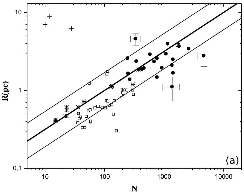
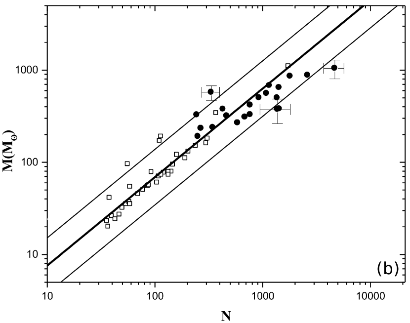
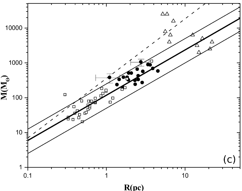
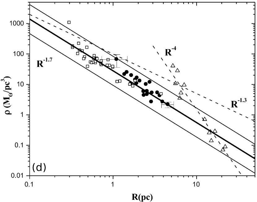
Figure 4: Comparing our objects (filled circles) with embedded clusters (open squares) studied by LL (03) and other samples. Representative error bars are used in a few data points, for illustration. (a): Radius of the cluster as a function of number of members. Our sample, as well as the embedded clusters follow the same dependence $R\propto N^{0.5}$ (thick line) found for the stellar clusters (asterisks) studied by Carpenter (2000). Thin lines indicate the limits suggested by Adams et al. (2006). The results obtained by Piskunov et al. (2007) for three objects of our sample (crosses) are used to illustrate differences on the cluster size definition. (b): Mass of the cluster as a function of number of members showing the same dependence $M\propto N^{1}$ for our sample and embedded clusters (thick line), with limits scaled by a factor $\sim$ 2 (thin lines). (c): Mass-radius dependence showing a mean distribution of M $\sim$ 118 R^1.3 (tick line) that spreads by a factor 2 (thin lines). The parameters of massive (“leak”) exposed clusters (triangles) are also plotted, as well as the dependence $M=359R^{1.7}$ suggested by Pfalzner (Pfalzner 2011 (2011)) for the embedded clusters (dashed line). (d): Volumetric density as a function of radius, showing the dependence $\rho$ = 28 R^-1.7 presented by our sample and LL (03) data (thick line), limited by thin lines that are scaled by a factor 2. Dashed lines represent the relations proposed by Pfalzner (Pfalzner 2011 (2011)).

5 Comparative Analysis

We investigate possible correlations among the cluster characteristics by comparing the structural and fundamental parameters, respectively from Table 1 and Table 2.

First, the correlations among mass, radius and number of members are compared to similar relations obtained by Adams et al. (2006) and Pfalzner (Pfalzner 2011 (2011)) using cluster properties from other works. In Sect. 5.4 the structural parameters (obtained on basis of surface density) are compared among each other, and Sect. 5.5 presents the relations with age.

5.1 Radius

Figure 4a shows the cluster radius distribution as a function of number of members (the same as fig.2 from Adams et al. 2006). Our sample is compared with 14 stellar clusters listed by Carpenter (2000), and 34 embedded clusters from LL (03), which have available size (radius in pc).

In order to illustrate the different cluster size definitions discussed in Sect. 3.2, we also plot the cluster radius ($R_{t}$) and the respective number of members ($N_{1}$) that were obtained by Piskunov et al. for three of our clusters (NGC 2362, NGC 6604, and Stock 13). It can be noted that the relation $R_{t}\times N_{1}$ (crosses in Fig. 4a) is incompatible with the distribution of the other samples, possibly due to the fact that Kharchenko et al. (2005) and citePiskunov 2007 study different stellar groups that encompass our clusters (see Sect. 3.2).

We verified that 52% of our sample follows the dependence R =0.1N^0.5 that is the same relation proposed by Adams et al. (2006) for the clusters listed by Carpenter (2000). Two of our clusters, NGC 6604 and Trumpler 18, as well as three clusters from LL (03) (NGC 2282, Gem 1, and Gem 4) also follow this trend, but scaled up by a factor 1.7, which is the superior limit suggested by Adams et al. (2006) for the distribution of cluster size as a function of N.

Coinciding with most of the LL (03) clusters, 33% of our sample are distributed along the lower curve in Fig. 4a that is similar to the Carpenter (2000) sample, but scaled down by a factor 1.7.

Lynga 14 appears bellow this correlation, suggesting that its membership is larger than the expected number of members, when compared to other clusters having same size. This characteristic is also noted for some clusters from LL (03), in particular S 106.

We also evaluate for our sample the commonly used half-mass radius $r_{1/2}$, which encloses half of the total mass of the cluster. Considering that we do not determine individual mass for each member of the clusters, their observed radial mass distribution cannot be established. In order to have an approximate estimation of $r_{1/2}$, we adopted the integrated mass distribution M(r) given by Adams et al. (2006):

$$\frac{M(r/r_{o})}{M_{tot}}=\bigg{[}\frac{(r/r_{o})^{a}}{\big{(}1+(r/r_{o})\big{)}^{a}}\bigg{]}^{p}$$ (7)

where $r_{o}$ is the scale length that we assume to be the radius of the cluster. The validity of using Eq.7 for our sample was checked for Lynga 14, Collinder 205 and Hogg 10, for which we could estimate the observed M(r) and were used as test cases. The “virial” model, used by Adams et al. (2006) in the simulations for N=100 members, has coefficients (a=3 and p $\sim$ 0.41) that seem to well reproduce the radial profile of the checked clusters. We verified that these simulations provide a ratio of $r_{1/2}/r_{o}$ of about 60-63%.

By adopting the relation $r_{1/2}$ = 0.615 $r_{o}$, we obtain the range of 0.69 - 2.5 pc for the half-mass radius estimated in our sample. We compared this result to the study that Adams et al. (2006) developed for NGC 1333, which model is most like the N=100 simulations with “cold” starting states (a=2 and p $\sim$ 0.55) and gives $r_{1/2}$ = 0.117 to 0.238 for $r_{o}$=0.3 to 0.4 pc. The relation $r_{1/2}/r_{o}$ is about 40-60% in this case, which is probably due to the fact that our clusters are more evolved than the embedded phase.

5.2 Mass

Figure 4b shows the relations between mass and number of members. The LL (03) sample has a dependence M = a N^1.0, where a = 0.6 ${}^{+0.6}_{-0.3}$, which means that they are distributed between the lines scaled (up and down) by a factor 2. Our objects also follow this dependence.

It is interesting to note that the clusters NGC 2282, Gem 1, and Gem 4, from LL (03), are found above the superior limit of the distribution. The same occurs for our clusters Trumpler 18 and NGC 6604, which showed a similar trend in the R $\times$ N plot (Fig. 4a).

The reason for a deviation of the expected relation is that these objects are different of most of the clusters. They have a smaller number of low-mass members, which is confirmed by their flat IMF ($\chi<$ 0.4). In the opposite sense, NGC 6178 and Stock 16 are found below the lower limit curve, being compatible with their steep IMF ($\chi>$ 1.4).

In order to discuss if these differences could be interpreted as formation condition, as proposed by Adams et al. (2006), or differently if they are related to a time sequence, as suggested by Pfalzner (Pfalzner 2011 (2011)), we compare the relations between mass and radius. The thick line in Fig. 4c shows that our sample has the same dependence obtained by fitting the LL (03) data: M = 118 R^1.3.

Figure 4c also displays the data of the “leaky” massive clusters studied by Pfalzner (Pfalzner 2011 (2011)), who proposed that these objects would be the ending of a time sequence. However, the mass-radius dependence M $\sim$ 359 R^1.7 (dashed line), which Pfalzner (Pfalzner 2011 (2011)) used to illustrate the suggested time sequence, is steeper than the distribution of LL (03) clusters.

Instead of confirming a sequence that ends in the exposed massive clusters, our results show that clusters from Pfalzner (Pfalzner 2011 (2011)) having radius $>$ 10 pc follow the same M vs. R relation presented by LL (03) data and also our sample. On the other hand, the massive clusters with R $<$ 10 pc are found above the upper line in Fig. 4c, similar to Lynga 14 and S 106 (LL (03)), which differences we interpret to be more likely due to different formation conditions.

5.3 Volumetric density

By assuming a spherical distribution, we estimated the volumetric density, defined by $\rho=3M/(4\pi R^{3})$, which is plotted in Fig. 4d as a function of radius. For both samples: our clusters and those from LL (03), we found a similar relation $\rho=28R^{-1.7}$. This is quite similar to the results obtained by Camargo et al. (2010) that find $\rho\propto R^{-1.92}$.

Pfalzner (Pfalzner 2011 (2011)) used a different dependence $\rho\sim 100R^{-1.3}$ to represent the LL (03) data, that were compared to the relation $\rho\propto R^{-4}$ obtained for the massive exposed clusters (dashed lines in Fig. 4c). However, the distribution of our clusters, as well as LL (03) data, does not agree with the mass vs. density relation proposed by Pfalzner (Pfalzner 2009 (2009, 2011)). As suggested in Sect. 5.2, the large massive clusters seem to follow the same trend of our clusters, while those with R $<$ 10 pc are scaled up by a factor larger than 2.

5.4 Surface density

Were analysed the structural parameters looking for correlations among the clusters themselves, and to verify a possible relation between the cluster and its environment. Hatched areas in Fig. 5 illustrate the trends that were found for most of the clusters.

Excepting for Trumpler 28, the observed average density of the cluster ($<n_{*}>$) increases with the background density ($\sigma_{bg}$), as shown in Fig. 5a. This indicates that dense clusters are found in dense background fields.

Considering that N increases with R (see Fig. 4a) it is expected an anti-correlation of $<n_{*}>$ vs. R, which is indeed noted in Fig. 5b. By consequence, $\sigma_{bg}$ also appears anti-correlated with R.

Core density ($\sigma_{0}$) is another structural parameter that also diminishes when cluster radius increases, but a considerable dispersion is seen in Fig. 5c, where almost six clusters are out of the observed trend.

In spite of the fact that R is not expected to be related to the cluster distance (D), Fig. 5d shows a trend of R increasing with D. This is not surprising, since the similar angular sizes of our objects lead to large linear size (given in parsec) for more distant clusters.

We plot in Fig. 5e the anti-correlation between core radius (r_c) and $\sigma_{0}$ that is observed for most of the clusters, excepting Lynga 14 and NGC 3590. The core parameters also showed some trends when compared with other structural parameters, like the correlation between $\sigma_{0}$ and $\delta_{c}$ (density contrast); and r_c/R (ratio of core-size to cluster radius) decreasing with the raise of $\sigma_{0}$.

The evaluation of structural parameters is unprecedented for most of our objects, but our results are comparable with those available in the literature for other clusters. We verified that the ranges of values obtained by us are compatible with several kind of young clusters like: NGC 6611, an embedded and dynamically evolved cluster (Bonatto, Santos Jr. & Bica (2006)); NGC 4755, a post-embedded cluster (Bonatto et al. (2006)); the low-mass open clusters NGC 1931, vdB 80, BDSB 96 and Pismis 5 (Bonatto & Bica , 2009a); NGC 2239, a possible ordinary open cluster (Bonatto & Bica, 2009b ); and the dissolving clusters NGC 6823 (Bica, Bonatto & Dutra, (2008)), Collinder 197, vdB 92 (Bonatto & Bica, BBica2010 (2010)) and Trumpler 37 (Saurin, Bica & Bonatto, SBB2012 (2012)).

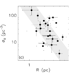
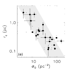
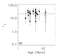
Figure 5: Comparing structural parameters: (5a) background density vs. average density. Cluster radius compared to (5b) average density; (5c) core density; and (5d) distance. (5e) core radius vs. core density. Age correlations with: (5f) core density; (5g) the fraction of cluster members showing excess in the K-band; and (5h) E(B-V). Dotted lines indicate respectively A${}_{V}\sim$ 1 mag and the limit of f${}_{K}=$ 20%. Triangles are used to indicate objects with two options of age (filled symbols correspond to the first choice, listed in Table 2).

5.5 Age

It would be expected that $\sigma_{0}$ should decrease with age once the members of older clusters could have had time to disperse, diminishing its surface stellar density. However no clear trend is observed in Fig. 5f, which displays different symbols to indicate objects that have two options of age, but only one of them was adopted.

The fraction of stars having large E(H-K), f_K, is expected to be related to age because of the colour excess in the K-band traces circumstellar matter, which is indicative of youth, as mentioned in Sect. 4.1 (Lada et al. (1996)). Figure 5g shows the distribution of f_K as a function of age, with a dotted line indicating the f_K = 20% limit, above which objects younger than 5 Myr are supposed to be found. Most of our objects have f${}_{K}>$ 20%, but three of the youngest clusters are below this limit, showing no correlation of age with f_K.

Probably this lack of correlation is due to the fact that some of our clusters have a mixing of populations, which means: part of the members is $<$ 4 Myr, while others are 4 - 10 Myr.

On the other hand, the lack of correlation is also found for Stock 16 that has f_K = 30% and mean age of 7.0${}^{+8.0}_{-6.5}$ Myr. An explantion is a possible field-stars contamination in the number of objects with K-band excess in the colour-colour diagram, mainly those having 0.1 $<$ (J-H)_o $<$ 0.3 mag. In the colour-magnitude diagram, these stars are counted in the range of ages older than 20 Myr, but should not be considered. The large error bars on both, age and f_K estimation, give us only a qualitative analysis of the relation between these parameters.

Age is also expected to be related with other parameters such as colour excess. Since E(B-V) is indicative of visual extinction, it can be used to infer how embedded the cluster is, and by consequence to verify the youth of the cluster. In fact, Fig. 5h shows three of the youngest objects ($<$ 5 Myr) appearing above the line representing E(B-V) = 0.3 mag, which means A${}_{V}>$ 1 mag. However, five other young clusters are below this limit, which indicates that they are not deeply embedded. For this reason, we concluded that there is no correlation between age and E(B-V) for our sample.

6 Summary of the results and conclusions

We determined the structural parameters as a function of superficial density and radial distribution profile of a sample of 21 clusters, selected on basis of their youth and intermediate distance. A statistical procedure using colour-magnitude criteria provided a double-checked decontamination of field-stars. The remaining stars were considered members and their observed colours were used to more accurately determine the visual extinction affecting the cluster. The unreddened colours were compared with theoretical isochrones in the CMD aiming to confirm distance and age. The same was done to determine individual masses, based on the cluster members position compared to evolutionary tracks.

In principle, centrally concentrated clusters should be the youngest ones since they would not had enough time to disperse. In fact, most of our clusters show this characteristic. However, the constrained range of ages in our sample impeaches us to be more conclusive about differences or similarities on the evolution of the studied clusters.

We conclude that all the 21 studied clusters are very similar, probably due to the selection criteria choosing restricted ranges of size, distance and age. By consequence, there is no large variation on number of members, radius and mass of the clusters. On the other hand, the galactic distribution of the objects causes differences among the clusters environments.

When compared with other young clusters (LL (03), Carpenter 2000), our sample follows the same trends, but has larger radius and lower volumetric density. This means a less concentrated distribution of members that may be related to the expected spatial dispersion, when the cluster gets older.

The distinction between star clusters and associations has been discussed in several works. Following the definitions presented by LL (03), our clusters are classified as stellar groups because they have more than 35 physically related stars and their mass density exceeds 1 M_⊙/pc^-3. Since our objects are optically visible, they cannot be considered embedded clusters. Even considering the large error bars on the age estimation, the mean age of the clusters ($\sim$ 5 Myr) is a clear indication that our sample is formed by young stellar associations.

We also checked for our sample the relation between age and crossing time ($\tau_{cr}$), following Gieles & Portegies Zwart (2011), for instance. They proposed a criterion in which bound systems (open star clusters) would have age/$\tau_{cr}>1$ and unbound systems would have age/$\tau_{cr}<1$. For this test, we adopted the crossing time defined by: $\tau_{cr}=\frac{2R}{\sigma_{V}}$, where R is the cluster radius and the stellar velocity dispersion is given by: $\sigma_{V}=\sqrt{\frac{GM}{R}}$, according to Saurin, Bica & Bonatto (SBB2012 (2012)).

We verified that none of our clusters has stars with age that exceeds the crossing time. Therefore, they probably would evolve like stellar associations. If the error bars on the age/$\tau_{cr}$ calculations are considered, only Lynga 14 could evolve as an open cluster. This result is in agreement with the suggestion by LL (03) and Pfalzner (Pfalzner 2009 (2009)), for instance, that few star clusters are expected to be bound. However, it must be kept in mind that these are qualitative conclusions, due to the large uncertainties on age estimation.

Our sample fulfils the caveat between the samples of embedded and exposed clusters studied by Pfalzner (Pfalzner 2011 (2011)). However, our results do not confirm the mass-radius or density-radius dependences suggested by her.

In fact, we verified that massive clusters from Pfalzner (Pfalzner 2011 (2011)) are distributed in two groups. Those with large sizes, lower masses, and intermediate ages (4 - 10 Myr) follow the same trends shown by embedded clusters (LL (03)), as well as our sample. The younger massive clusters ($<$ 4 Myr) studied by Pfalzner (Pfalzner 2011 (2011)) have lower sizes and higher masses, appearing out of the correlations shown in Fig. 4, as well as Lynga 14 (this work) and S 106 (LL (03)). As proposed by Adams et al. (2006), the differences among these clusters could be interpreted as formation condition.

An interesting perspective of the present work is to increase the studied sample by including other clusters having larger radius (4 - 10 pc), which could complet the gap between our clusters and the sample of massive clusters.

Appendix A Plots of the entire sample

All plots used in the analysis of structural and fundamental parameters are displayed in this Appendix. Figures A1 and A2 show the stellar surface-density maps and the distribution of the stellar density as a function of radius (same as Fig. 1).

Figures A3 to A7 present colour-colour and colour-magnitude diagrams in the left panel (same as Fig. 2). The centre and right panels show respectively the histogram of age and the mass distribution (same as Fig. 3).

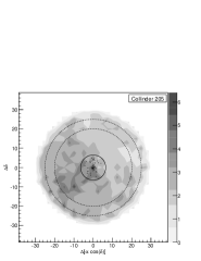
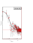
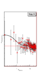
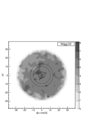
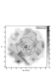
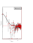
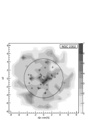
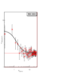
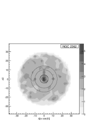
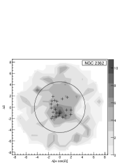
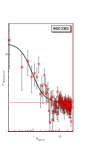
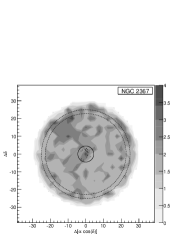
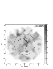
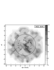
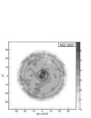
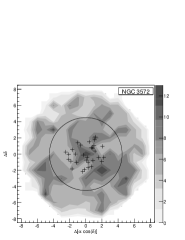
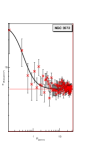
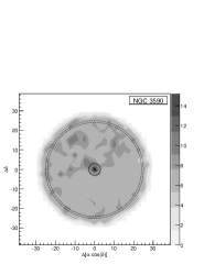
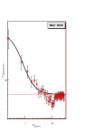
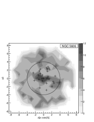
Figure 6: Left: Stellar surface-density map ($\sigma$ (stars/arcmin²)) obtained for the region of 30 arcmin around the clusters. The comparison field-stars area is indicated by dashed lines, while the full line indicates the cluster area. Centre: a zoom of the $\sigma$ map indicating by crosses the position of objects with membership probability P$>$70%. Right: The distribution of the stellar density as a function of radius. The best fitting of observed radial density profile, indicated by the full line, was obtained by using the model from King (1962). A dashed line indicates the background density ($\sigma_{bg}$).

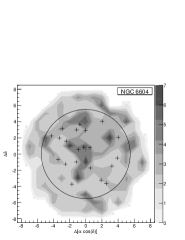
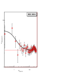
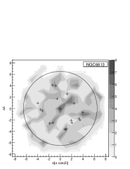
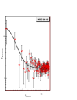
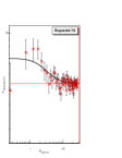
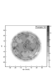
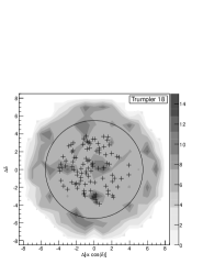
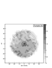
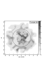
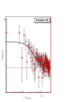
Figure 7: Same as Fig. A1

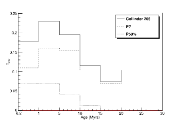
Figure 8: Left panels: Colour-colour and colour-magnitude diagrams. The MS and the ZAMS are indicated by full lines, while the locus of giant stars is represented by a dotted line. Reddening vectors from Rieke & Lebofsky (1985) are shown by dot-dashed lines. The isochrones and evolutionary pre-MS tracks from Siess et al. (2000). Cluster members are indicated by open diamonds (P50) and dots (P?). Centre: Age distribution of clusters members (thick line) showing the contribution of P50 (dotted line) and P? (dashed line) objects. Right: Observed mass distribution indicated by crosses with error bars. The thick line represents the mass function $\phi$(m) fitting.)

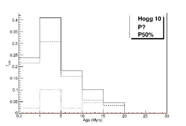
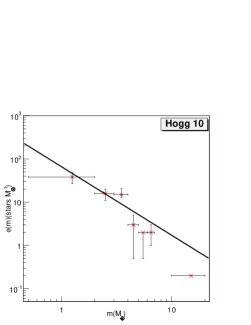
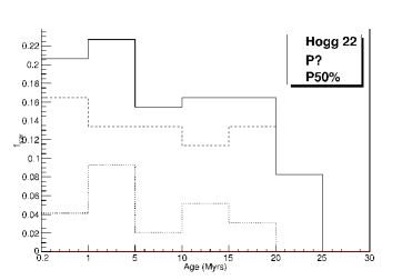
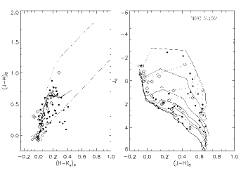
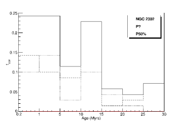
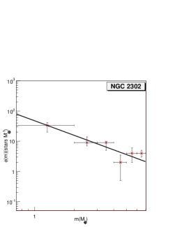
Figure 9: The same as Fig A.3.

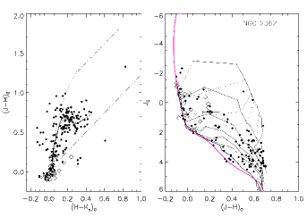
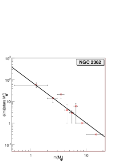
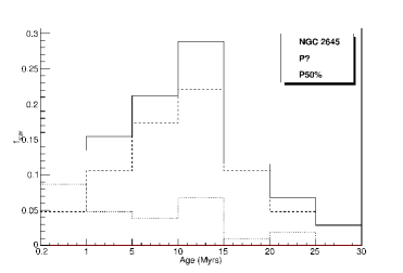
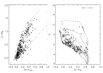
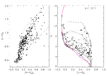
Figure 10: The same as Fig A.3.

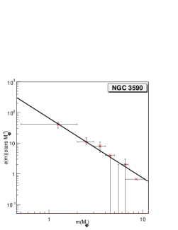
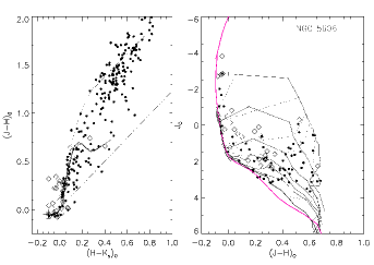
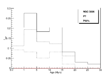
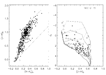
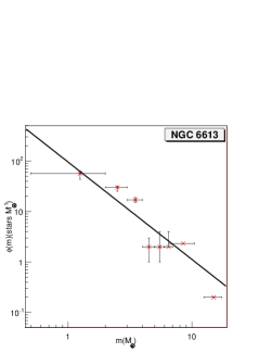
Figure 11: The same as Fig A.3.

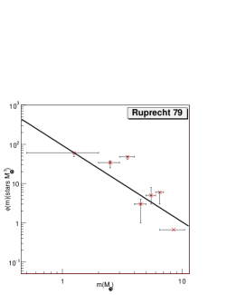
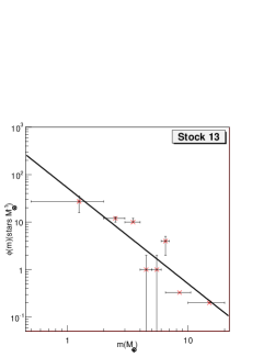
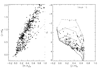
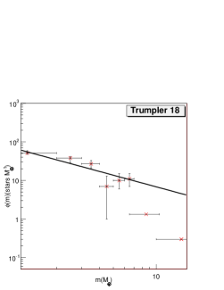
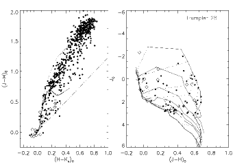
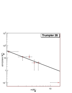
Figure 12: The same as Fig A.3.