Study of the 3D Coronal Magnetic Field of Active Region 11117 Around the Time of a Confined Flare Using a Data-Driven CESE–MHD Model

Abstract

We apply a data-driven MHD model to investigate the three-dimensional (3D) magnetic field of NOAA active region (AR) 11117 around the time of a C-class confined flare occurred on 2010 October 25. The MHD model, based on the spacetime conservation-element and solution-element (CESE) scheme, is designed to focus on the magnetic-field evolution and to consider a simplified solar atomsphere with finite plasma $\beta$. Magnetic vector-field data derived from the observations at the photoshpere is inputted directly to constrain the model. Assuming that the dynamic evolution of the coronal magnetic field can be approximated by successive equilibria, we solve a time sequence of MHD equilibria basing on a set of vector magnetograms for AR 11117 taken by the Helioseismic and Magnetic Imager (HMI) on board the Solar Dynamic Observatory (SDO) around the time of flare. The model qualitatively reproduces the basic structures of the 3D magnetic field, as supported by the visual similarity between the field lines and the coronal loops observed by the Atmospheric Imaging Assembly (AIA), which shows that the coronal field can indeed be well characterized by the MHD equilibrium in most time. The magnetic configuration changes very limited during the studied time interval of two hours. A topological analysis reveals that the small flare is correlated with a bald patch (BP, where the magnetic field is tangent to the photoshpere), suggesting that the energy release of the flare can be understood by magnetic reconnection associated with the BP separatrices. The total magnetic flux and energy keep increasing slightly in spite of the flare, while the computed magnetic free energy drops during the flare with an amount of $\sim 10^{30}$ erg, which seems to be adequate to provide the energy budget of the minor C-class confined flare.

1 Introduction

The magnetic field holds a central position within solar research such as sunspots, coronal loops, prominences, and spectacular solar phenomena like flares and coronal mass ejections (CMEs). It has been commonly accepted that the energy released by solar flare (which is usually up to the order of $10^{32}$ erg during the major events) must be sourced from magnetic field of the active region since all the other possible energy sources are completely inadequate (Priest, 1987). To help quantitative understanding the solar explosive phenomena such as flare and CMEs, it is essential to get the knowledge of the amount of free magnetic energy and its temporal variation during the events. Magnetic reconnection is attributed by most flare models to the basic mechanism for energy conversion rapidly from the magnetic field into the kinetic and thermal counterparts (Priest & Forbes, 2002; Shibata & Magara, 2011). To locate where magnetic reconnection is prone to happen and produce flare needs the three-dimensional (3D) coronal magnetic field, by which the important topological and geometrical features that are favorable sites for reconnection, e.g., the null point, the separatrices or more commonly the quasi-separatrix layers (Priest & Forbes, 2002; Titov et al., 2002; Longcope, 2005), can then be found. Unfortunately, the 3D magnetic field in the corona is very difficult to be directly observed, although information of the 3D geometrical configuration of the field lines can be partially reconstructed by the method of stereoscopy using coronal loops observed in different aspect angles in the EUV and X-ray wavelengths (see living review by Aschwanden, 2011). Up to the present, a routinely direct measurement of the solar magnetic field on which we can rely is mainly restricted to the solar surface, i.e., the photosphere (there are only a few cases available with the measurements of the chromospheric and coronal fields, e.g., Solanki et al., 2003; Lin et al., 2004).

With in hand the observed magnetic field on the photosphere, there are several ways to study the evolution of 3D magnetic field in the corona. One of them is the well-known model of field extrapolation from the magnetogram, especially, the nonlinear force-free (NLFF) field extrapolation (Wiegelmann, 2008; Schrijver et al., 2008; DeRosa et al., 2009). As the solar corona is dominated by the magnetic field environment with very small plasma $\beta$ (the ratio of gas pressure to magnetic pressure), the force free model is usually valid and serves as a good approximation for the low corona (but above the photosphere) in a near-static state. A variety of numerical codes have been developed to implement the force-free field extrapolation in the past decade (e.g., Wheatland et al., 2000; Wiegelmann, 2004; Amari et al., 2006; Jiang & Feng, 2012). These methods have been applied to analyze the magnetic structures of the active regions, the electric current distributions, energy budget of the eruptions, etc (Régnier & Canfield, 2006; Guo et al., 2008; Thalmann & Wiegelmann, 2008; Jing et al., 2010; Valori et al., 2012; Sun et al., 2012), with success made, such as reproducing the field lines comparable with the observed coronal loops (e.g., Wiegelmann et al., 2012) and extrapolating complex flux rope which is believed to be associated with the filament channel (e.g., Canou & Amari, 2010). However, it should be noted that the success is still limited when applied to realistic solar data (Schrijver et al., 2008; DeRosa et al., 2009; Schrijver, 2009), which is mainly because of the intrinsic non-force-freeness in the field close to the photosphere (Metcalf et al., 1995). Thus the observed data can generally not provide a consistent boundary condition for the model based on an exact force-free assumption, and some ad hoc preprocessing (to remove the force in the raw magnetogram) is usually made to prepare the vector magnetograms for the extrapolation codes (Wiegelmann et al., 2006).

Another method is using data-driven magnetohydrodynamics (MHD) model which is more general than the force-free one (Wu et al., 2006, 2009; Wang et al., 2008; Jiang et al., 2010; Fan et al., 2011, 2012). This is because in the MHD model, nonlinear dynamic interactions of the magnetic field and plasma flow field are treated in a self-consistent way, in which the near force-free state of the coronal magnetic field is included. A first data-driven MHD model was developed by Wu et al. (2006) for simulating the evolution of active regions. In their original work, the initial setup of the model is established by seeking a MHD equilibrium started from an arbitrarily prescribed plasma and a potential magnetic field based on the Solar and Heliospheric Observatory (SOHO)/MDI magnetogram at a given time. Then a time-series of MDI magnetograms observed afterward were continuously inputted at the bottom boundary to drive the above field to respond to the changes on the photosphere. In particular, the procedure of continuously feeding observed data on the bottom boundary is made to be self-consistent by a projected-characteristic method (e.g., Nakagawa, 1981; Wu & Wang, 1987).

If in an ideal or strict condition, this dynamic process of the data-driven model can indeed be regarded as evolution of the corona. However, in the reality, there are still many difficulties and problems in using a data-driven MHD model to study the active region evolution. First of all is the lack of observations for the photospheric parameters of plasma such as the surface flow velocity, which is important boundary information for the driving process (Abbett et al., 2004; Welsch et al., 2004). This is especially essential by regarding that at the photosphere the magnetic field may be dominated by the dense plasma (with high $\beta$), and the field lines anchored in the photosphere can usually be considered as line-tied by the photospheric plasma because of the high electric conductivity (Priest, 1987; Mikic & Linker, 1994; Solanki et al., 2006). This means that the field-line footpoints are passively advected by the plasma flow which itself is induced in the convection zone below. Without the information of the surface flow, response of the coronal field lines driven by photospheric footpoint-motion cannot be fully followed. This encourages people to recover the photospheric flow velocity from the time-varying magnetograms by using local correlation tracking technique or similar methods (e.g., see Chae, 2001; Welsch et al., 2004; Démoulin & Pariat, 2009). The second problem comes from the cadence of the observed data which is generally too low for a data-driven model that needs a highly continuous data flow. To address this problem, Wu et al. (2006) simply used a time-linear interpolation on the 96-minute cadence MDI magnetograms to provide the data needed at each time step (about 6-second used by Wu et al., 2006) of the model. This obviously over-simplifies the real evolution of the photospheric field which is very time-nonlinear, but it may be the only choice one can made . In view of these two problems, it may be more practical to construct independent MHD equilibrium for each one of the magnetograms and consider these successive equilibria as the continuous time-evolution of the corona, as done by Wu et al. (2009); Fan et al. (2011).

For the third problem, it is difficult to couple the photospheric and the coronal plasma in a single model because of the highly stratified plasma, of which the parameters, i.e., the density and temperature change drastically by several orders of magnitude within an extremely thin layer (the chromosphere and transition region) above the photosphere due to some kind of unknown coronal heating process. As a realistic model with inputted magnetic field data observed on the photosphere, it is required to describe the behavior of the magnetic field in this stratified environment with plasma $\beta$ varying from $>1$ (the photosphere) to $\ll 1$ (the corona). However, this challenges greatly the numerical scheme and computational resource to treat the transition region and additionally, one may need to incorporate the complicated thermodynamic processes of the real corona, such as the thermal conduction and radiative losses (e.g., see models by Abbett, 2007; Fang et al., 2010). We note that in the works of (Wu et al., 2006, 2009; Wang et al., 2008; Fan et al., 2011), only the photospheric or near-photosphere plasma is considered in the models and thus these models are mainly used for studying the evolution of photospheric parameters, such as the plasma flow, the Poynting flux, the current helicity and some other non-potential parameters at the photosphere level. The evolution of the 3D coronal magnetic field, on the other hand, was rarely studied by using these models because of the unjustified high-$\beta$ and dense plasma environment. This is due to the reason mentioned above that a coupled modeling of the photospheric and coronal fields is still computationally prohibitive.

In this work we will use the data-driven MHD model to study the 3D coronal field within a low plasma–$\beta$ condition. The numerical model is developed following our previous work (Jiang et al., 2011), which has been devoted to a validation of the CESE–MHD method for reconstructing the 3D coronal fields using a semi-analytic force-free field solution proposed by Low & Lou (1990). We will study the 3D magnetic field and its evolution of active region NOAA AR 11117 around the time of a small C-class flare happened on 2010 October 25, observed by SDO/AIA with a time-series of vector-magnetograms recorded by SDO/HMI. While the 3D magnetic field of the same active region has been studied by Sun et al. (2010) and Tadesse et al. (2012) using the NLFFF model, this is the first study we apply the CESE–MHD model to realistic solar data. Similarly assuming that the evolution of the coronal magnetic field in active region can be described by successive equilibria (e.g., Régnier & Canfield, 2006; Wu et al., 2009; Sun et al., 2012; Tadesse et al., 2012), we use each vector-magnetogram of the data set to get a snapshot MHD equilibrium and study the temporal evolution of the field by a series of these equilibria. This method is justified by considering that the evolution of the active region, driven by the photospheric motion with flow speed on the order of several km s^-1, is sufficiently slow compared with the speed of the coronal magnetic field relaxing to equilibrium, which is up to thousands of km s^-1 (Antiochos, 1987; Seehafer, 1994). It is also valid for the present studied objective, the AR 11117, which shows no major changes of the magnetic field in the chosen time period.

The remainder of the paper is organized as follows. In Section 2 we give a brief description of the CESE–MHD model. Magnetic field data used for driven the model is described in Section 3. The modeling result for the AR 11117 is presented in Section 4, including a qualitative inspection of the the 3D magnetic configurations, topological analysis of the field at the flare site, as well as study of the magnetic energy budget and current distribution. Finally we draw conclusions and give some outlooks for future work in Section 5.

2 The Data-Driven CESE–MHD Model

In a nutshell, what we intend to solve is a set of MHD equilibria of which each is consistent with a snapshot of magnetic field observed on the photosphere. We thus start from an arbitrarily initial field, e.g., a potential or linear force-free field, with a plasma and input at the bottom of the model the vector magnetogram to drive the system away from its initial state and then let the system relax to a new equilibrium. The numerical model follows our previous work (Jiang et al., 2011). Since the computation is focused on the magnetic field and its dynamics with plasma in the low corona, here we use a simplified solar atmosphere with a low plasma $\beta$ and a uniform constant temperature. Thus the numerical scheme need only to handle the plasma density $\rho$, the flow velocity ${\mathbf{v}}$ and the magnetic field ${\mathbf{B}}$. The MHD equations are written as follows:

$$\frac{\partial\rho}{\partial t}+\nabla\cdot(\rho{\mathbf{v}})=0,$$

$$\rho\frac{D\mathbf{v}}{Dt}=-{\bf\nabla}p+{\mathbf{J}}\times{\mathbf{B}}+\rho{\mathbf{g}}+\nabla\cdot(\nu\rho\nabla\mathbf{v})-\nu_{f}\rho{\mathbf{v}},$$

$$\frac{\partial\mathbf{B}}{\partial t}=\nabla\times(\mathbf{v}\times\mathbf{B}).$$ (1)

In these equations: ${\mathbf{J}}$ is the electric current; $p$ is the gas pressure given by $p=\rho RT_{0}$ where $R$ is gas constant and $T_{0}$ is the constant temperature; ${\mathbf{g}}$ is the solar gravity and is assumed to be constant as its photospheric value since we simulate the low corona with height of about $100$ Mm from the photosphere. A small kinematic viscosity $\nu$ with a value of $\sim\Delta x^{2}/\Delta t$ ($\Delta x$, $\Delta t$ are respectively the grid spacing and the time step in the numerical scheme) is added for consideration of numerical stability.

Different from the equations used in Jiang et al. (2011), here we include an additional frictional force $-\nu_{f}\rho{\mathbf{v}}$ to deal with the problem that in some odd places near the magnetogram (i.e., the bottom) the plasma velocity is prone to be accelerated to extremely high due to very large gradients or some kind of uncertainties intrinsically contained in the observed data. This is because the data is very intermittent in the observed magnetograms, which usually show a large number of small-scale polarities and even apparent discontinuities, and these features cannot be adequately resolved by the grid resolution. We find that such problems can severely restrict the time step and slow the relaxation process of the entire system, even making the computation unmanageable. It should be noted that including the friction force is only an ad hoc choice for numerical consideration in the case of dealing with the original data in the model. Alternatively, one can perform certain smoothing on the original magnetograms beforehand to remove noise and decrease large gradients in the raw data. This, however, may erase some of the important parasitic polarities around the major sunspots and also probably change the locations of the polarity inversion lines (PILs), which could influence the analysis of the local field configurations responsible for small-scale energy dissipation near the photosphere (e.g., the small flare in the present study). Also there is magnetic flux loss and the energy content of the field may be affected, if the vertical component of the magnetogram is modified (Metcalf et al., 2008). Although the field at the coronal base ought to be smoother than the photospheric field because of the field expansion from the high-$\beta$ to the low-$\beta$ regions, in which way such smoothness can be modeled is still problematic. To this end, it is prudent not to smooth the original magnetograms and thus we use the frictional force to control the above-mentioned problem in the numerical computation. We have tried different values for the frictional coefficient $\nu_{f}$ and adopt a optimized one $\nu_{f}=1/(50\Delta t)$, which can control the plasma flow in a reasonable level, i.e., the flow speed is suppressed under the maximum Alfvén speed but not too small. Our tests show that the adjustment of $\nu_{f}$ affects the MHD relaxation process but gives almost the same final solution. Finally, no explicit resistivity is included in the magnetic induction equation, since the numerical diffusion can lead to topological changes of the field when necessary.

The above equation system (2) is solved by our CESE–MHD code (Jiang et al., 2010). The CESE method deals with the 3D governing equations in a substantially different way that is unlike traditional numerical methods (e.g., the finite-difference or finite-volume schemes). The key principle, also a conceptual leap of the CESE method, is treating space and time as one entity. By introducing the conservation-element (CE) and the solution-element (SE) as the vehicles for calculating the spacetime flux, the CESE method can enforce conservation laws both locally and globally in their natural spacetime unity form. Compared with many other numerical schemes, the CESE method can achieve higher accuracy with the same mesh resolution and provide simple mathematics and coding free of any type of Riemann solver or eigendecomposition. For more detailed descriptions of the CESE method for MHD simulations including the multi-method control of the well-known $\nabla\cdot\mathbf{B}$ numerical errors, please refer to our previous work, e.g., Feng et al. (2006, 2007), Jiang et al. (2010) and Jiang et al. (2011). We use a non-uniform grid within the framework of a block-structured, distributed-memory parallel computation. The grid configuration is depicted in Figure 1. Specifically, the whole computational volume is divided into blocks with different spatial resolution, and the blocks are evenly distributed among the CPU processors. In the $x$–$y$ plane, i.e., the plane parallel with the photosphere, the blocks have the same resolution. In the vertical direction, resolutions of the blocks are decreased with height, e.g., near the photosphere, the grid spacing matches the resolution of the magnetogram and up to the top of the model box, the grid spacing is increased by four times. As shown by Figure 1, at a height of only 10 Mm the magnetic field has become far less intermittent, i.e., much smoother than that at the photosphere. Thus using this non-uniform mesh can affect the computational accuracy little compared with a uniform mesh, but can save significant computational resources.

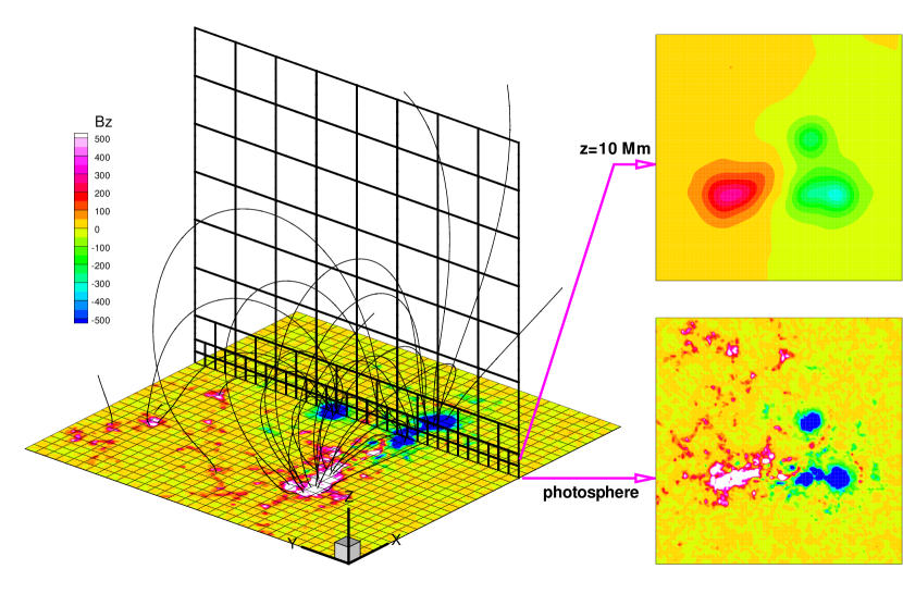
Figure 1: The configuration of the computational grid. The entire volume is divided into blocks and each block has $8\times 8\times 8$ cells. In the left panel, two slices through the volume are plotted to show the structure of the blocks, which are outlined by the black grid lines; the bottom contour map represents $B_{z}$ on the photosphere and the curved lines show the potential field lines. The right panels show the 2D contour images of $B_{z}$ sliced at $z=0$ and $z=10$ Mm (locations in the 3D grid are shown by the arrows).

The initial configuration of the simulation consists of a potential field matching the vertical component of the magnetogram and a plasma in hydrostatic equilibrium in the solar gravitational field. The potential field is obtained by a Green’s function method (e.g., Metcalf et al., 2008). The plasma density is given by $\rho(z)=\rho_{0}\exp(-z/H)$ where $H$ is the pressure scale height $H=RT_{0}/g$ and $z=0$ denotes the photosphere. Nondimensionalization of the parameters is same as Jiang et al. (2011) and Figure 2 shows a typical configuration of the parameters along a vertical line through the computation volume at the strong magnetic region. It is noteworthy that the plasma $\beta$ can be large in the relatively weak field region and thus the intrinsic force in the vector magnetogram can be self-consistently balanced by the plasma in the MHD relaxation process. This is unlike the force-free model, as aforementioned (see Section 1), which generally cannot deal with the observed data directly. The boundary conditions are also very similar to those used in Jiang et al. (2011): the bottom boundary is fed with the observed vector magnetogram incrementally in tens of Alfvén time until the observed data is fully matched, and all other boundaries are set by the non-reflecting boundary conditions. Besides, the flow velocity on the bottom is set by extrapolation from the neighboring inner grid. This has a function to increase the communication between the magnetogram and the computational volume (Valori et al., 2007).

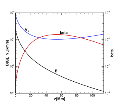
Figure 2: Typical configurations of the magnetic field strength $B$, the Alfvén speed $V_{\rm A}$ and the plasma $\beta$ along a vertical line through the computation volume.

3 Data

Active region NOAA AR 11117 was observed by SDO from 2010 October 20 to 2010 November 2, mainly during Carrington Rotation 2102. On 2010 October 25, it was crossing the central meridian of the solar disk with latitude of $22^{\circ}$ as shown in the full-disk HMI and AIA images (Figure 3). On this date solar activity was dominated by AR 11117 with many small B-class flares observed and near the end of the day, a C2.3-class flare happened. NOAA records indicate that the event began in soft X-rays (SXRs) which were detected by the GOES (Geostationary Operational Environmental Satellite) 15 satellite at 22:06 UT, reaching a peak at 22:12 UT and ending at 22:18 UT (see Figure 4). As observed by AIA (see Figure 6), the central part of the active region shows distinct brightenings at the flare peak time and the flare is confined in rather low altitude without inducing major changes in the coronal loops or eruptions.

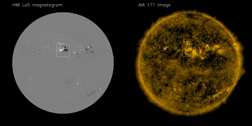
Figure 3: Full-disk SDO/HMI line-of-sight (LoS) magnetogram (left) and full-disk SDO/AIA 171 Å image. Both images are obtained at the same time of 22:12 UT on 2010 October 25, and have been co-aligned. AR 11117 is outlined by the white rectangle on the images.

Figure 4: GOES soft-X ray flux from 20:00 UT to 24:00 UT on 2010 October 25 in the wavelength range of 1–8 Å. Horizontal dotted line indicates the C-minor flare class and the vertical dotted line indicates the peak time of the flux.

We select a set of vector magnetograms for AR 11117 which were taken by HMI around the flare peak time with a cadence of roughly half an hour. The data is de-rotated to the disk center, the field vectors are transformed to Heliographic coordinates with projection effect removed and finally remapped to a local Cartesian coordinate using Lambert equal area projection. For a detailed processing of the HMI vector magnetograms please refer to http://jsoc.stanford.edu/jsocwiki/VectorMagneticField. Specifically, six magnetograms taken at 21:00, 21:36, 22:00, 22:12, 22:36, and 23:00 UT, respectively, are used for the simulation. Figure 5 shows examples of the vector magnetograms before and at the flare peak time (the gray image shows the vertical component $B_{z}$ and the arrows indicate the transverse field). There are four regions with flux greater than 1000 G concentrated in areas of about 10 arcsec square and these regions are manifested as four main sunspots observed in the AIA 4500 Å (white light) image. Strong shear of the transverse field can be seen near the image center, with the vector almost parallel to the PIL (see the regions where the color of the vectors changes while their directions are nearly the same). The original resolution of the magnetogram is about 0.5 arcsec ($\sim 360$ km) per pixel and we bin the data to 1 arcsec pix^-1 for our simulation with a field of view of $256\times 256$ arcsec² ($184\times 184$ Mm²). The height of the computational box is set to 160 arcsec ($115$ Mm). To reduce the side and top boundary influence, the following analysis of the results is performed on a subvolume with $200\times 128\times 100$ arcsec³ centered in the full computational domain.

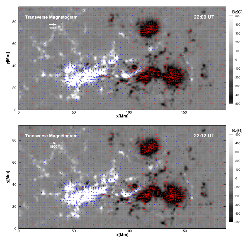
Figure 5: Vector magnetograms for AR 11117 at time of 22:00 and 22:12. The gray images represent $B_{z}$ with a saturation level of $\pm 500$ G. The tangential fields are shown by the vectors (plotted at every third pixel point) with blue color in the positive $B_{z}$ region and red in the negative $B_{z}$ region.

4 Results

4.1 Comparison with AIA Loops

The high-resolution coronal loops observed by SDO/AIA in the wavelength of 171 Å give us a proxy of the magnetic field-line geometry (see the left column of Figure 6) and also a good constraint for the magnetic field model. In the middle column of Figure 6 we show some selected magnetic field lines of the model results. In these images, the yellow lines represent the magnetic field lines and the background contours outline the vertical component of the magnetogram. For a visual comparison with the observed coronal loops, we plot the figures side-by-side with the AIA 171 Å images observed at the same time. The field lines are selected roughly according to the visible bright loops and the angle of view of the MHD results is co-aligned with the AIA image. As shown from an overview of the figures, the simulated field lines resemble quite well the observed loops, especially at the central region of the AR where the field lines are sheared strongly. This means that the field there is very non-potential. The potential fields at each time are shown in the third column of Figure 6. Compared with the potential field lines, the MHD field lines exhibit some twists, although not strong, implying the existence of field-line-aligned currents (i.e., currents along the field lines). We find that there are features well reproduced by the MHD model but failed to be recovered by the potential model, for example, the structures pointed out by the white arrows in the figure. Reconstruction of these features, obviously needing variation of the field-line connectivities from those of the initial potential field, demonstrates that our model can indeed reconstruct the 3D magnetic topology which is implied in the observed transverse field.

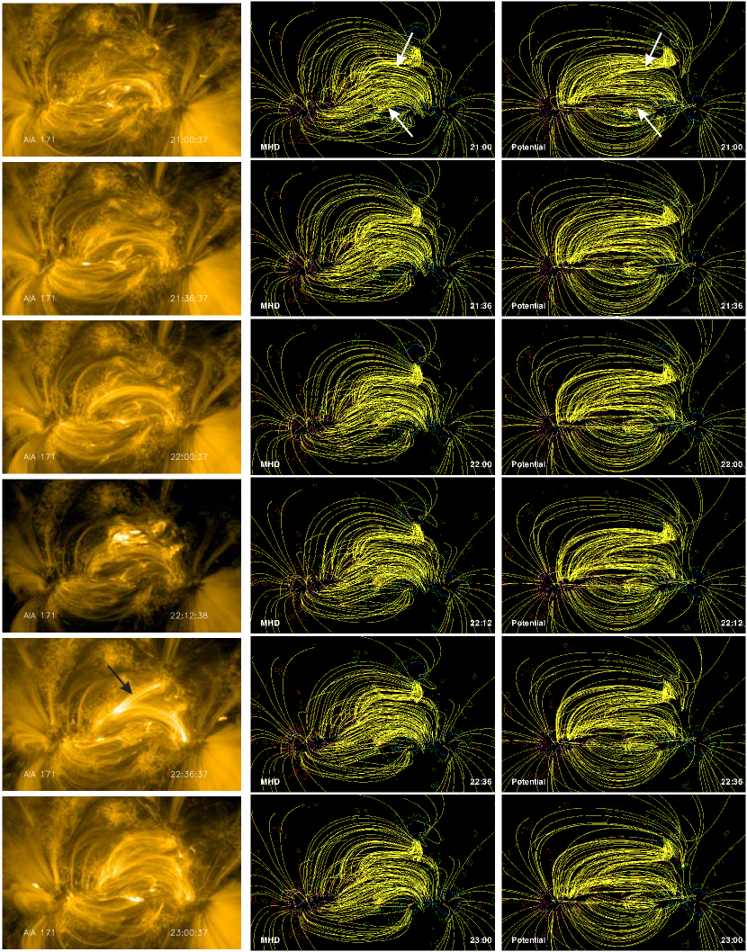
Figure 6: Comparison of the modeled field lines with SDO/AIA 171 Å image for AR 11117. The left column is the AIA images, the middle column is the selected magnetic field lines from the MHD results. Also the potential field lines are plotted in the last column. The field lines in all the panels are traced from the same footpoints on the photosphere and the color contours of photospheric $B_{z}$ are plotted on the background.

By comparison we conclude that within this AR, the MHD model gives much better results than the potential field model. Although during this time interval some small changes can be recognized in the loops and the MHD field lines, it is difficult to find any variation in the magnetic topology around the time of flare from 22:00 to 22:12. This means that the flare-related reconnection takes place at rather small scale and low height near the photosphere (as indicated by the analysis of magnetic topology in the following section). It can be clearly seen in the AIA image at 22:36 there are two groups of loops with much more brightness than the other loops, and the MHD model appears to fail to reproduce the groups in the north (i.e., the loops pointed out by the black arrow in the image, note that this group of loops is difficult to find in all the other AIA images in the figure). This may be due to that the central part of the active region is very dynamic after the flare since hot plasma from the chromosphere ‘evaporated’ to the post-flare loops, thus cannot be well described by the quasi-static state which we have sought.

4.2 Topological Analysis of the Flare Location

It has been thought that flare is plausible to take place in the regions with strong variation of the field line connectivity (e.g., Mandrini et al., 1995; Demoulin et al., 1997). Such regions are called quasi-separatrix layers (QSLs), which are generalized from the concept of magnetic separatrices where the field-line linkage (or connectivity) is discontinuous (Priest & Démoulin, 1995; Demoulin et al., 1996). To locate the QSLs in the 3D coronal field, Titov et al. (2002) introduced a so-called squashing factor ($Q$) to quantify the change of the field linkage basing on the field-line mapping. For the corona field, the mapping is defined from one photospheric footpoint $(x,y)$ of a given field line to the other photospheric footpoint $(X(x,y),Y(x,y))$, which is also called the magnetically conjugate footpoint. Then the squashing factor is given by

$$Q=\frac{a^{2}+b^{2}+c^{2}+d^{2}}{|ad-bc|}$$ (2)

where

$$a=\frac{\partial X}{\partial x},\ \ b=\frac{\partial X}{\partial y},\ \ c=\frac{\partial Y}{\partial x},\ \ d=\frac{\partial Y}{\partial y}.$$ (3)

Producing a map of $Q$ factor is a robust way to find the topological elements (including both the QSLs and the separatrices) in the 3D magnetic field, but its calculation is a computational intensive work because field lines are required to be traced from not only each point but also its neighboring points to estimate the derivatives of the field line mapping. We thus use the following algorithm: first, field line from each grid point $(i,j)$ on the bottom surface is traced either forward or backward and location of the other (conjugate) footpoint is denoted by $(X(i,j),Y(i,j))$; then at each grid point a centered difference involving with its neighboring four grid points $(i-1,j),(i+1,j),(i,j-1),(i,j+1)$ is used to approximate the elements needed by $Q$, i.e.,

$$a=\frac{X(i+1,j)-X(i-1,j)}{2\Delta x},$$

$$b=\frac{X(i,j+1)-X(i,j-1)}{2\Delta y},$$

$$c=\frac{Y(i+1,j)-Y(i-1,j)}{2\Delta x},$$

$$d=\frac{Y(i,j+1)-Y(i,j-1)}{2\Delta y}.$$ (4)

where $\Delta x$ and $\Delta y$ are the grid spacings. To avoid the numerical uncertainties of tracing field lines with very small structures near the photosphere (i.e., structures smaller than the grid resolution), we raise the bottom surface by three pixels (about 2 Mm) above the photosphere in the computation. This might smooth out some very fine structures in the $Q$ map but the basic topological features remain since they depend mainly on the large-scale current distribution (Titov & Démoulin, 1999). As suggested by Titov et al. (2002), it is also useful to compute the expansion-contraction degree ($K$) which is defined by the ratio of the normal components of the magnetic field at the two ends of the field lines. While the factor $K$ has similar function to locate the QSLs as $Q$, it is much simpler to compute than the latter, and may be more reliable since its computation is free of the numerical errors of the finite difference in Equation (4.2).

Considering that the magnetic field is nearly steady with time, we only compute the QSLs for a single frame. Figure 7 depicts the $Q$ and $K$ maps (panel (b) and (d)) for the magnetic field at 22:12 and compares with the AIA image at the same time. We use a logarithmic scale since the squashing factor becomes abruptly very large inside ths QSLs (e.g., Titov et al. (2002) defined the QSL as a region with $Q\gg 2$). Note that there are data gaps in the maps because the field lines there are opened, i.e., with ends of the lines reaching the side or top boundaries of the computational volume. As shown by the $Q$ and $K$ maps, the structures associated with data abrupt change, i.e., the QSLs, are consistent between both maps. The whole structure of the $Q$ map is rather complicated and may deserve a comprehensive study, while here we put our focus on analyzing the relation of the flare location (outlined by the dashed rectangle on the AIA image) with the QSLs. Indeed, the flare location is clearly co-spatial with the QSL of which the squashing factor reaches $\sim 10^{3}$ (see the region in the dashed rectangle in the $Q$ map). Then why is this subregion has a strong change of magnetic connectivity? In the same figure, we show the vector magnetogram (panel (e)) and the field lines (panel (f)) in the same but a little larger subregion outlined by the black rectangle in panel (c). The vector magnetogram and the field lines reveal that underlying the flare region a bald patch (BP) is located at the central portion of a long PIL (enhanced by the thick white line in panels (e) and (f)). By its definition, BP is a portion of PIL with $({\mathbf{B}}\cdot\nabla)B_{z}>0$, which means the horizontal field at PIL crosses from the negative to positive $B_{z}$ (Titov et al., 1993; Bungey et al., 1996), just oppossite to the normal case. In the middle of the BP, the transverse field is nearly parallel with the PIL, suggesting that it is not a single BP but fragments into two parts. BP can also be defined as the locations where the magnetic field is tangent to the photosphere, and the continuous set of field lines that graze the surface at the BP form two separatrix surfaces which separates three different topological regions. The separatrix field lines are shown in Figure 7 (f) and with 3D views in Figure 8. Several studies have demonstrated that BP can be correlated with flares and even CMEs due to the BP separatrices, in which strong current sheets can be formed by photospheric motions or flux emergence and trigger reconnection (e.g., Aulanier et al., 1998; Fletcher et al., 2001; Mandrini et al., 2002; Wang et al., 2002). The topological analysis of the flare site here, thus, suggests that the AR 11117 flare can also be interpreted as a bald-patch flare (Aulanier et al., 1998; Delannée & Aulanier, 1999), and may provide an evidence in favor of reconnection along BP separatrices. The heights of the apexes of the BP separatrices is about $2\sim 3$ Mm, meaning that the flare happened rather low near the photosphere. However, in which way the current sheet is formed and how the reconnection is triggered are not clear and further study relying on higher-resolution and cadence data could be needed. For another evidence of the presence of the BP co-spatial with the flare, a curved dark feature near the flare location, shown by the arrows on the AIA image (see panel (a) of Figure 7), has the same shape with the field lines near the right end of the BP (indicated by the arrows in panel (f)). This can be well explained by the dip of field lines just above the BP, which can support dense cold plasma against gravity in the same way as filaments.

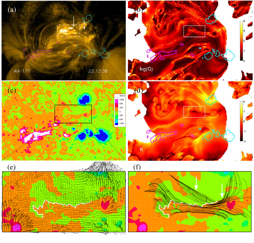
Figure 7: (a) The AIA 171 image at 22:12, with the contour lines plotted for the LoS photospheric field at $\pm 1000$ G and the dashed box showing the location of flare with loops brightened. (b) The squashing factor $Q$ in logarithmic scale; samely contours are plotted at $\pm 1000$ G for photospheric $B_{z}$ and the dashed box outlines the flare location. (c) The $B_{z}$ map with the flare location outlined by a black box which is enlarged in panel (e). (d) Same as (b) but for the expansion-contraction degree $K$. (e) The vector magnetogram in the flare location and the thick white line denotes the bald patch (BP). Panel (f) gives some examples of the field lines (i.e., the BP separatrix field lines) that are tangent to the photosphere at the BP (the thick white line).

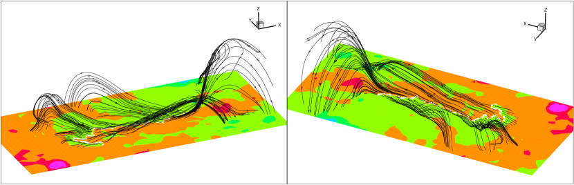
Figure 8: Different 3D views of the BP-separatrix field lines plotted in panel (f) of Figure 7. The BP is denoted by the thick white lines. The $z$–axis scale is doubled for a better view of the field lines.

4.3 Energy and current

In order to quantify the change of the field in the time series, we computed a set of parameters and summarized them in Table 1. They include the total unsigned magnetic flux $|\Phi|_{\rm tot}=\int_{S}|B_{z}|{\ \mathrm{d}}S$ (where $S$ represents the photosphere), the total unsigned current $|I|_{\rm tot}=\int_{S}|j_{z}|{\ \mathrm{d}}S$ (i.e., integral of the unsigned vertical current on the photosphere), the total energy $E_{\rm tot}=\frac{1}{8\pi}\int_{V}B^{2}dV$, the potential energy $E_{\rm pot}$, the free energy $E_{\rm free}=E_{\rm tot}-E_{\rm pot}$, and the ratio of free energy to potential energy. All these parameters are important to characterize the evolution of the coronal magnetic field. The first four parameters, i.e., the magnetic flux, the current, the total and the potential energies, all keep increasing with time in spite of the small flares. This is due to that the energy injected by emerging magnetic flux is larger than the energy released by the flares (e.g., Régnier et al., 2005; He et al., 2011). The total energy and the potential energy are on the order of $10^{32}$ erg which is a typical energy content of a medium-sized active region. Because of the non-potentiality of the field, the total energy $E_{\rm tot}$ is always higher than that of the potential field, which holds a energy minimum state with a given magnetic flux on the photosphere. It is commonly believed that the free magnetic energy plays a fundamental role in flares, because the source of the energy for the flare must be magnetic and only a fraction of the total magnetic energy, i.e., the free energy can be converted to the kinetic energy and radiation of flare (Priest & Forbes, 2002). Our computation shows that the free energy is on the order of $10^{31}$ erg (close to $10^{32}$ erg) which seems to suffice to power a moderate flare, and this energy initially increased like the total and potential energies before the C-class flare started at 22:06 UT. One should bear in mind that even the free energy is only partially involved with flares since the field after flares is still non-potential and nonlinear (e.g., see Schrijver, 2009). The energy released by the flare ought to be quantified by the change in free energy from immediately before to after the flare. Although the total energy increased even in the interval of the flare, the free energy dropped as expected at 22:12, i.e., the peak time of the flare, with a small amount of about $1.7\times 10^{30}$ erg. It has been estimated that for the largest flares up to X-class, the energy released are on the order of $10^{32}$ erg (e.g., Priest, 1981, 1987). Thus by a rough estimation, the decrease in the free energy of pre- and post-flare is actually adequate to power this minor flare, of which the energy needed is about several percents of the largest class. Nevertheless, caution is needed when estimating the energy budget of the flare by the drop of free energy in our modeling, since many aspects of the model and the specific approach may influence the results. We will discuss this in the conclusion section. In the last column of Table 1 we calculated a mean vector deviation between field ${\mathbf{b}}$ at each time with respect to the field ${\mathbf{B}}$ at time 21:00

$$e_{\rm m}=\frac{1}{M}\sum_{i}\frac{|{\mathbf{b}}_{i}-{\mathbf{B}}_{i}|}{|{\mathbf{B}}_{i}|}$$ (5)

where $i$ denotes the indices of all the pixels of the computational volume and $M$ is the total number of the pixels. As a metric monitoring the numerical variation of the field with the time, the very low values of $e_{\rm m}$ again show that the change of the field are rather small.

Time	$|\Phi|_{\rm tot}$[$10^{22}$ Mx]	$|I|_{\rm tot}$[$10^{13}$ A]	$E_{\rm tot}$[$10^{32}$ erg]	$E_{\rm pot}$[$10^{32}$ erg]	$E_{\rm free}$[$10^{31}$ erg]	$E_{\rm free}/E_{\rm pot}$	$e_{\rm m}$
21:00	1.60	4.77	4.80	4.04	7.66	0.19	0.00
21:36	1.63	4.80	4.95	4.18	7.69	0.18	0.09
22:00	1.65	4.84	5.05	4.27	7.78	0.18	0.11
22:12	1.66	4.92	5.09	4.33	7.61	0.18	0.10
22:36	1.68	4.96	5.21	4.41	7.95	0.18	0.11
23:00	1.70	5.05	5.28	4.50	7.79	0.17	0.13

Table 1: Variation of parameters with evolution of the field, see text for details.

In addition to the global energy content, we can also study the spatial distribution of the magnetic free energy, i.e., the locations of the free energy storage. As an example, for the magnetic field at time 22:00 we computed the vertical integration of the free energy

$$E_{\rm free}(x,y)=A\int\frac{{\mathbf{B}}^{2}-{\mathbf{B}}_{\rm pot}^{2}}{8\pi}{\ \mathrm{d}}z$$ (6)

where $A={\ \mathrm{d}}x{\ \mathrm{d}}y$, and plotted the distribution of $E_{\rm free}(x,y)$ on the horizontal plane (Figure 9). A sum of the energy $E_{\rm free}(x,y)$ in the images gives the total free energy listed in Table 1. Over the left image of Figure 9, the contour lines show the vertically integrated current density $\int|{\mathbf{J}}|{\ \mathrm{d}}z$ and the lines are color-coded with strength of the integrated current (increasing from black to white); Over the right image the strongest regions of $B_{z}$ of photospheric field are outlined by the contour lines ($\pm 1000$ G). It can be clearly seen that the distribution of the free energy is largely co-spatial with that of the current. This can be easily understood because the coronal free energy (or the non-potential energy) is actually stored in the current-carrying field (where non-potentiality is strong). On the other hand, as shown by the right image, the concentrations of free energy is not generally spatially-correlated with those of strongest magnetic flux. It should be noted that in the image there are some places with negative values of the vertically integrated free energy. This is physically valid since the there is no restriction that the energy density (and thus any sub-volume energy) must always be greater than that of the potential field, although a non-potential field must have a global energy content greater than the potential field (e.g., Mackay et al., 2011). In Figure 10 we plot the horizontal surface-integral of the total energy, the potential energy, and the free energy, e.g.,

$$E_{\rm free}(z)={\ \mathrm{d}}z\int\frac{{\mathbf{B}}^{2}-{\mathbf{B}}_{\rm pot}^{2}}{8\pi}{\ \mathrm{d}}x{\ \mathrm{d}}y$$ (7)

as functions of the height $z$. The total and the potential energies are predominantly located near the photosphere where the magnetic field strength is high, whereas the free energy (the red curve) is situated mainly above the photosphere in a range of 5 Mm to 30 Mm with its maximum at about 10 Mm. It is interesting to find that near the photosphere, the free energy is negative with a minimum value at the photosphere, which says that the observed vector field has a lower surface energy content than the potential field. This is, however, not surprising as we have noted that any sub-volume energy content of the non-potential field may be lower than potential energy.

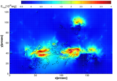
Figure 9: The images represent vertical integral of the free energy, showing the locations of free energy storage. The contour lines in the left panel represent the vertically integrated current density $\int|{\mathbf{J}}|{\ \mathrm{d}}z$ and the lines are color-coded with strength of the integrated current (increasing from black to white). The contour lines in the right panel represent $B_{z}$ on the photosphere with value of $\pm 1000$ G.

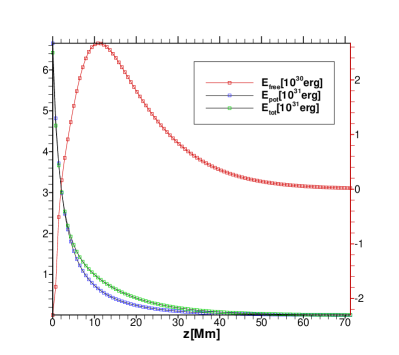
Figure 10: Variation of the horizontal surface integration of magnetic field energy along the $z$-axis. Note that the left vertical axis (black) indicates values for the $E_{\rm pot}$ and $E_{\rm tot}$ and the right vertical axis (red) indicates values for $E_{\rm free}$.

Electric current can characterize the non-potentiality of the field, e.g., the patterns of strong current concentration may serve as a proxy for the non-potential structures (e.g., the sigmoids) in the corona (Schrijver et al., 2008; Archontis et al., 2009; Sun et al., 2012). In particularly, the current structures are regions where reconnection may happen and magnetic energy is converted to thermal energy and heating, and thus creating hot emission. In Figure 11 we give examples of the synthetic images of the current which is computed by vertical integration of $J^{2}$ (i.e., $\int_{z}J^{2}{\ \mathrm{d}}z$, see Archontis et al. (2009)) and compared with the AIA 304 Å images. Since the term $J^{2}$ is proportional to the Joule heating term, thus it simulates but very roughly the hot emission. As can be seen in the figure, the strong current regions are indeed coincident with the regions with high intensity of emission. However, the result does not show any intensive current associated with the flare site. This may be because the current sheet in the BP separatrices is very thin and is failed to be resolved by the present grid resolution.

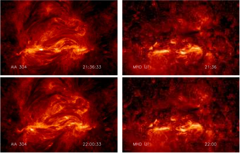
Figure 11: Left column is the AIA 304 Å image and right column is the synthetic images of current using vertical integral of $J^{2}$ computed by the MHD model.

5 Conclusions

In this work, we have applied the data-driven CESE–MHD model to investigate the 3D magnetic field of AR 11117 around the time of a C-class confined flare occurred on 2010 October 25. Similar to the field extrapolation method our model is designed to focus on the magnetic field, but its nonlinear dynamic interactions with plasma and finite gas pressure (denoted by plasma $\beta$) are also embedded, although simplified. Assuming that the dynamic evolution of the coronal magnetic field can be approximated by successive equilibria, we have solved a time sequence of MHD equilibria basing on a set of vector magnetograms for AR 11117 taken by SDO/HMI around the time of flare. By analyzing the computed 3D magnetic field along with the observation, we have the following results:

1. The model has qualitatively reproduced the basic structures of the magnetic field, as supported by the visual similarity between the field lines and the SDO/AIA loops, which shows that the coronal field can indeed be well characterized by the MHD equilibrium in most time. The magnetic field is very non-pontential with strong shear locally and some twists compared with the potential model. There are also some loops failed to be recovered by the MHD model, but only at the time set very near the happening of the flare. This means that the magnetic field is rather dynamic when the energy is suddenly released in a time-scale far shorter than that of relaxation by Alfvén speed.

2. The magnetic configuration changes very limited during the studied time interval of two hours, and the flare-related reconnection takes place at rather small scale and low height near the photosphere. The topological analysis reveals that the small flare is correlated with a BP and the energy dissipation can be understood by the reconnection associated with the BP separatrices. However, no intensive current is found in the flare site related with the BP separatrices. This may be because the current sheet associated with the separatrices is very thin and cannot be resolved by the present grid resolution. Further study exploiting the full resolution and high-cadense observations is required for explaining how the BP-flare is actived, e.g., where the current sheet is formed and how the reconnection is triggered.

3. Because of the continuous flux emergence, the total unsigned magnetic flux and current through the photosphere keep increasing (but very slightly) in spite of the flare. Although evolution of the total magnetic energy also exhibits the same tendency as that of the total magnetic flux, the sum of free energy for the computational volume drops when the flare happened, indicating that some of the non-potential energy is released by the flare. Our computation shows that the amount of the free energy loss is on the order of $10^{30}$ erg, which is adequate to power a minor C-class flare.

In summary, our model capture the basic features of the 3D magnetic field of the target active region both qualitatively and quantitatively, also the results give some hints on the trigger mechanism of the flare. Nevertheless, we remind the readers that the results, especially in the quantitative aspect, should be interpreted with caution because they can be influenced by many uncertainties in the modeling. The uncertainties also exist in other models of the similar kind, for example, the NLFF modeling, and even for the same model, different codes may produce very inconsistent results (Schrijver et al., 2008; DeRosa et al., 2009). The uncertainties may first come from measurement error of the HMI magnetogram data. For example, Sun et al. (2012) have estimated that the free energy content could be affected with several percents by the spectropolarimetric noise in the magnetogram; even such small error is large for the present case in which the flare may only release a very small fraction of the free energy. It should be noted that in the NLFF model the systematic error can be greater because of the force-free assumption and the preprocessing and smoothing of the original data. Although our model does not suffer from such preprocessed-related problem, the systematic uncertainties can still come from the simplified configuration of the solar atmosphere, the boundary conditions and the data interpolation from the original non-uniform grid to a uniform grid when computing the parameters. Especially the using of a low-$\beta$ plasma globally is far from the realistic case in which the solar atmosphere is highly stratified with much larger gas pressure near the photosphere. Furthermore the assumption of static state of the magnetic field is unjustified by the onset of the flare, which can drive the field lines very dynamic and make our computation unreliable, as discussed in the comparison of the MHD results with the AIA images. This is a much more basic problem (than the others aforementioned) encountered by any extrapolation of magnetic field with static or quasi-static models.

Future improvements merit to be made in several aspects. To increase the capability of adaptive resolving the small-scale structures can be realized hopefully by the aid of the adaptive-mesh-refinement technique. Exploiting more observations like the surface flows computed by the LCT-type methods can further constraint the model and provide important information for the realistic dynamic evolution of the magnetic field. More physics-based thermodynamic model for the solar atmosphere with stratified temperature will also be considered to couple the photosphere and corona, in order to model the behavior of the magnetic field in a highly stratified and inhomogeneous plasma with $\beta$ from $>1$ to $\ll 1$.

References

- Abbett (2007) Abbett, W. P. 2007, ApJ, 665, 1469
- Abbett et al. (2004) Abbett, W. P., Mikić, Z., Linker, J. A., McTiernan, J. M., Magara, T., & Fisher, G. H. 2004, Journal of Atmospheric and Solar-Terrestrial Physics, 66, 1257
- Amari et al. (2006) Amari, T., Boulmezaoud, T. Z., & Aly, J. J. 2006, A&A, 446, 691
- Antiochos (1987) Antiochos, S. K. 1987, ApJ, 312, 886
- Archontis et al. (2009) Archontis, V., Hood, A. W., Savcheva, A., Golub, L., & Deluca, E. 2009, ApJ, 691, 1276
- Aschwanden (2011) Aschwanden, M. J. 2011, Living Reviews in Solar Physics, 8, 5
- Aulanier et al. (1998) Aulanier, G., Démoulin, P., Schmieder, B., Fang, C., & Tang, Y. H. 1998, Sol. Phys., 183, 369
- Bungey et al. (1996) Bungey, T. N., Titov, V. S., & Priest, E. R. 1996, A&A, 308, 233
- Canou & Amari (2010) Canou, A. & Amari, T. 2010, ApJ, 715, 1566
- Chae (2001) Chae, J. 2001, ApJ, 560, L95
- Delannée & Aulanier (1999) Delannée, C. & Aulanier, G. 1999, Sol. Phys., 190, 107
- Demoulin et al. (1997) Demoulin, P., Bagala, L. G., Mandrini, C. H., Henoux, J. C., & Rovira, M. G. 1997, A&A, 325, 305
- Demoulin et al. (1996) Demoulin, P., Henoux, J. C., Priest, E. R., & Mandrini, C. H. 1996, A&A, 308, 643
- Démoulin & Pariat (2009) Démoulin, P. & Pariat, E. 2009, Advances in Space Research, 43, 1013
- DeRosa et al. (2009) DeRosa, M. L., Schrijver, C. J., Barnes, G., Leka, K. D., Lites, B. W., Aschwanden, M. J., Amari, T., Canou, A., McTiernan, J. M., Régnier, S., Thalmann, J. K., Valori, G., Wheatland, M. S., Wiegelmann, T., Cheung, M. C. M., Conlon, P. A., Fuhrmann, M., Inhester, B., & Tadesse, T. 2009, ApJ, 696, 1780
- Fan et al. (2011) Fan, Y. L., Wang, H. N., He, H., & Zhu, X. S. 2011, ApJ, 737, 39
- Fan et al. (2012) Fan, Y.-L., Wang, H.-N., He, H., & Zhu, X.-S. 2012, Research in Astronomy and Astrophysics, 12, 563
- Fang et al. (2010) Fang, F., Manchester, W., Abbett, W. P., & van der Holst, B. 2010, ApJ, 714, 1649
- Feng et al. (2006) Feng, X., Hu, Y., & Wei, F. 2006, Sol. Phys., 235, 235
- Feng et al. (2007) Feng, X., Zhou, Y., & Wu, S. T. 2007, ApJ, 655, 1110
- Fletcher et al. (2001) Fletcher, L., López Fuentes, M. C., Mandrini, C. H., Schmieder, B., Démoulin, P., Mason, H. E., Young, P. R., & Nitta, N. 2001, Sol. Phys., 203, 255
- Guo et al. (2008) Guo, Y., Ding, M. D., Wiegelmann, T., & Li, H. 2008, ApJ, 679, 1629
- He et al. (2011) He, H., Wang, H., & Yan, Y. 2011, J. Geophys. Res., 116, 1101
- Jiang et al. (2011) Jiang, C., Feng, X., Fan, Y., & Xiang, C. 2011, ApJ, 727, 101
- Jiang & Feng (2012) Jiang, C. W. & Feng, X. S. 2012, ApJ, 749, 135
- Jiang et al. (2010) Jiang, C. W., Feng, X. S., Zhang, J., & Zhong, D. K. 2010, Sol. Phys., 267, 463
- Jing et al. (2010) Jing, J., Tan, C., Yuan, Y., Wang, B., Wiegelmann, T., Xu, Y., & Wang, H. 2010, ApJ, 713, 440
- Lin et al. (2004) Lin, H., Kuhn, J. R., & Coulter, R. 2004, ApJ, 613, L177
- Longcope (2005) Longcope, D. W. 2005, Living Reviews in Solar Physics, 2, 7
- Low & Lou (1990) Low, B. C. & Lou, Y. Q. 1990, ApJ, 352, 343
- Mackay et al. (2011) Mackay, D. H., Green, L. M., & van Ballegooijen, A. 2011, ApJ, 729, 97
- Mandrini et al. (1995) Mandrini, C. H., Demoulin, P., Rovira, M. G., de La Beaujardiere, J.-F., & Henoux, J. C. 1995, A&A, 303, 927
- Mandrini et al. (2002) Mandrini, C. H., Démoulin, P., Schmieder, B., Deng, Y. Y., & Rudawy, P. 2002, A&A, 391, 317
- Metcalf et al. (2008) Metcalf, T. R., DeRosa, M. L., Schrijver, C. J., Barnes, G., van Ballegooijen, A. A., Wiegelmann, T., Wheatland, M. S., Valori, G., & McTtiernan, J. M. 2008, Sol. Phys., 247, 269
- Metcalf et al. (1995) Metcalf, T. R., Jiao, L., McClymont, A. N., Canfield, R. C., & Uitenbroek, H. 1995, ApJ, 439, 474
- Mikic & Linker (1994) Mikic, Z. & Linker, J. A. 1994, ApJ, 430, 898
- Nakagawa (1981) Nakagawa, Y. 1981, ApJ, 247, 707
- Priest (1981) Priest, E. R. 1981, Solar Flare Magnetohydrodynamics (London: Gordon and Breach)
- Priest (1987) —. 1987, Solar magneto-hydrodynamics., ed. Priest, E. R.
- Priest & Démoulin (1995) Priest, E. R. & Démoulin, P. 1995, J. Geophys. Res., 100, 23443
- Priest & Forbes (2002) Priest, E. R. & Forbes, T. G. 2002, A&A Rev., 10, 313
- Régnier & Canfield (2006) Régnier, S. & Canfield, R. C. 2006, A&A, 451, 319
- Régnier et al. (2005) Régnier, S., Fleck, B., Abramenko, V., & Zhang, H. 2005, in Chromospheric and Coronal Magnetic Fields, Vol. 596, 61
- Schrijver (2009) Schrijver, C. J. 2009, Advances in Space Research, 43, 739
- Schrijver et al. (2008) Schrijver, C. J., DeRosa, M. L., Metcalf, T., Barnes, G., Lites, B., Tarbell, T., McTiernan, J., Valori, G., Wiegelmann, T., Wheatland, M. S., Amari, T., Aulanier, G., Démoulin, P., Fuhrmann, M., Kusano, K., Régnier, S., & Thalmann, J. K. 2008, ApJ, 675, 1637
- Seehafer (1994) Seehafer, N. 1994, A&A, 284, 593
- Shibata & Magara (2011) Shibata, K. & Magara, T. 2011, Living Reviews in Solar Physics, 8, 6
- Solanki et al. (2006) Solanki, S. K., Inhester, B., & Schüssler, M. 2006, Reports on Progress in Physics, 69, 563
- Solanki et al. (2003) Solanki, S. K., Lagg, A., Woch, J., Krupp, N., & Collados, M. 2003, Nature, 425, 692
- Sun et al. (2012) Sun, X., Hoeksema, J. T., Liu, Y., Wiegelmann, T., Hayashi, K., Chen, Q., & Thalmann, J. 2012, ApJ, 748, 77
- Sun et al. (2010) Sun, X., Hoeksema, J. T., Wiegelmann, T., Hayashi, K., & Liu, Y. 2010, AGU Fall Meeting Abstracts, A1607
- Tadesse et al. (2012) Tadesse, T., Wiegelmann, T., Inhester, B., & Pevtsov, A. 2012, Sol. Phys., 60
- Thalmann & Wiegelmann (2008) Thalmann, J. K. & Wiegelmann, T. 2008, A&A, 484, 495
- Titov & Démoulin (1999) Titov, V. S. & Démoulin, P. 1999, A&A, 351, 707
- Titov et al. (2002) Titov, V. S., Hornig, G., & Démoulin, P. 2002, J. Geophys. Res., 107, 1164
- Titov et al. (1993) Titov, V. S., Priest, E. R., & Demoulin, P. 1993, A&A, 276, 564
- Valori et al. (2012) Valori, G., Green, L. M., Démoulin, P., Vargas Domínguez, S., van Driel-Gesztelyi, L., Wallace, A., Baker, D., & Fuhrmann, M. 2012, Sol. Phys., 278, 73
- Valori et al. (2007) Valori, G., Kliem, B., & Fuhrmann, M. 2007, Sol. Phys., 245, 263
- Wang et al. (2008) Wang, A. H., Wu, S. T., Liu, Y., & Hathaway, D. 2008, ApJ, 674, L57
- Wang et al. (2002) Wang, T., Yan, Y., Wang, J., Kurokawa, H., & Shibata, K. 2002, ApJ, 572, 580
- Welsch et al. (2004) Welsch, B. T., Fisher, G. H., Abbett, W. P., & Regnier, S. 2004, ApJ, 610, 1148
- Wheatland et al. (2000) Wheatland, M. S., Sturrock, P. A., & Roumeliotis, G. 2000, ApJ, 540, 1150
- Wiegelmann (2004) Wiegelmann, T. 2004, Sol. Phys., 219, 87
- Wiegelmann (2008) —. 2008, J. Geophys. Res., 113, 3
- Wiegelmann et al. (2006) Wiegelmann, T., Inhester, B., & Sakurai, T. 2006, Sol. Phys., 233, 215
- Wiegelmann et al. (2012) Wiegelmann, T., Thalmann, J. K., Inhester, B., Tadesse, T., Sun, X., & Hoeksema, J. T. 2012, Sol. Phys., 67
- Wu et al. (2009) Wu, S. T., Wang, A. H., Gary, G. A., Kucera, A., Rybak, J., Liu, Y., Vrśnak, B., & Yurchyshyn, V. 2009, Advances in Space Research, 44, 46
- Wu et al. (2006) Wu, S. T., Wang, A. H., Liu, Y., & Hoeksema, J. T. 2006, ApJ, 652, 800
- Wu & Wang (1987) Wu, S. T. & Wang, J. F. 1987, Computer Methods in Applied Mechanics and Engineering, 64, 267