Joint Detection/Decoding Algorithms for Nonbinary LDPC Codes over ISI Channels

Abstract

This paper is concerned with the application of nonbinary low-density parity-check (NB-LDPC) codes to binary input inter-symbol interference (ISI) channels. Two low-complexity joint detection/decoding algorithms are proposed. One is referred to as max-log-MAP/X-EMS algorithm, which is implemented by exchanging soft messages between the max-log-MAP detector and the extended min-sum (EMS) decoder. The max-log-MAP/$X$-EMS algorithm is applicable to general NB-LDPC codes. The other one, referred to as Viterbi/GMLGD algorithm, is designed in particular for majority-logic decodable NB-LDPC codes. The Viterbi/GMLGD algorithm works in an iterative manner by exchanging hard-decisions between the Viterbi detector and the generalized majority-logic decoder (GMLGD). As a by-product, a variant of the original EMS algorithm is proposed, which is referred to as $\mu$-EMS algorithm. In the $\mu$-EMS algorithm, the messages are truncated according to an adaptive threshold, resulting in a more efficient algorithm. Simulations results show that the max-log-MAP/$X$-EMS algorithm performs as well as the traditional iterative detection/decoding algorithm based on the BCJR algorithm and the QSPA, but with lower complexity. The complexity can be further reduced for majority-logic decodable NB-LDPC codes by executing the Viterbi/GMLGD algorithm with a performance degradation within one dB. Simulation results also confirm that the $\mu$-EMS algorithm requires lower computational loads than the EMS algorithm with a fixed threshold. These algorithms provide good candidates for trade-offs between performance and complexity.

I Introduction

Nonbinary low-density parity-check (NB-LDPC) codes were first introduced by Gallager based on modulo arithmetic [1]. In [2], Davey and Mackay presented a class of NB-LDPC codes defined over the finite field $\mathbb{F}_{q}$. They also introduced a Q-ary sum-product algorithm (QSPA) for decoding NB-LDPC codes. NB-LDPC codes outperform their binary counterparts when used in the channels with burst errors or combined with higher-order modulations. However, the applications of NB-LDPC codes are limited due to their high decoding complexity. To reduce the decoding complexity, a more efficient QSPA based on fast Fourier transform (FFT-QSPA) was proposed in [3][4]. To further reduce the decoding complexity, extended min-sum (EMS) algorithms were proposed in [5][6]. The EMS algorithm in [6] was re-described in [7] as a reduced-search trellis algorithm, called $M$-EMS algorithm. Also presented in [7] are two variants of the $M$-EMS algorithm, called $T$-EMS algorithm and $D$-EMS algorithm, respectively. For majority-logic decodable NB-LDPC codes, different low-complexity decoding algorithms have been proposed [8][9]. Different construction methods of NB-LDPC codes have been proposed in the literature, see [10, 11, 12] and the references therein.

The inter-symbol interference (ISI) is a common phenomenon in high-density digital recording systems and wireless communication systems [13]. Different equalizers have been proposed in the literature [14, 15, 16, 17, 18, 19, 20, 21, 22, 23]. Since the invention of the turbo codes [24], the rediscovery of the LDPC codes [1], and most importantly, the success of the applications of turbo principle to equalizations [19][25][26], many works have been done to apply turbo principles to coded ISI channels [27, 28, 29, 30, 31, 32, 33], where binary convolutional codes, turbo codes or LDPC codes are usually considered as the “outer codes” of the serial concatenated system. However, few works are available for the NB-LDPC coded ISI channels. An example is given in Appendix showing that nonbinary may be more suitable to combat inter-symbol interference.

In this paper, we investigate reduced complexity detection/decoding algorithms for NB-LDPC coded ISI channels. Two low-complexity joint detection/decoding algorithms are proposed. For general NB-LDPC coded ISI channels, we propose the max-log-MAP/$X$-EMS algorithm, in which the detector and the decoder are implemented with the max-log-MAP algorithm and the $X$-EMS algorithm, respectively. In this algorithm, the detector takes as input the soft extrinsic messages from the decoder and delivers as output the soft extrinsic messages of each coded symbol; the decoder takes as input the messages from the detector and feeds back to the detector the soft extrinsic messages of each coded symbol. Simulations results show that the max-log-MAP/$X$-EMS algorithm performs as well as the traditional iterative detection/decoding algorithm based on the BCJR algorithm and the QSPA, but with reduced complexity. Meanwhile, a variant of the original $T$-EMS algorithm is proposed, which is referred to as $\mu$-EMS. The threshold of the $\mu$-EMS algorithm is adaptive and hence can be matched to channel observation. Simulation results show that the proposed $\mu$-EMS algorithm is more effective than the original $T$-EMS algorithm when applied to coded ISI channels. For majority-logic decodable NB-LDPC coded ISI channels, a further complexity-reduced joint detection/decoding algorithm is proposed, referred to as Viterbi/GMLGD algorithm, which is based on the Viterbi algorithm and the generalized majority-logic decoding (GMLGD) algorithm [9]. In the Viterbi/GMLGD algorithm, the Viterbi detector takes as input the messages from the decoder and delivers as output the hard-decision sequence; the decoder takes as input the hard-decision sequence from the detector and feeds back to the detector the estimated messages of each coded symbol. Simulations results show that the Viterbi/GMLGD algorithm suffers from a performance degradation within one dB compared with BCJR/QSPA. These algorithms provide good candidates for trade-offs between performance and complexity.

The organization of this paper is as follows. Section II introduces the considered system model. Also given in Section II is the quantization algorithm to initialize the detector. The max-log-MAP/$X$-EMS algorithms and the Viterbi/GMLGD algorithm are described in Section III and Section IV, respectively. Complexity comparisons and simulation results are given in Section V. Section VI concludes this paper.

II NB-LDPC Coded ISI Channel

II-A NB-LDPC Codes

Let $\mathbb{F}_{q}$ be the finite filed with $q=2^{m}$ elements. A NB-LDPC code $\mathcal{C}_{q}[N,K]$ is defined as the null space of a sparse nonbinary parity-check matrix $\mathbf{H}=[h_{i,j}]_{M\times N}$, where $h_{i,j}\in\mathbb{F}_{q}$. A vector $\underline{v}=(v_{0},v_{1},v_{2},\cdots v_{q-1})\in\mathbb{F}_{q}^{N}$ is a codeword if and only if $\mathbf{H}\underline{v}^{T}=0$. For convenience, we define the two index sets as follows:

$\mathcal{N}_{i}=\{j:0\leq j\leq N-1,h_{i,j}\neq 0\}$   for each row $i$ of $\mathbf{H}$

and

$\mathcal{M}_{j}=\{i:0\leq i\leq M-1,h_{i,j}\neq 0\}$   for each column $j$ of $\mathbf{H}$.

II-B ISI Channel Model

The ISI channel of order $L$ is characterized by a polynomial

$$f(D)=f_{0}+f_{1}D+f_{2}D^{2}+\cdots+f_{L}D^{L},$$ (1)

where the coefficients $f_{l}\in\mathbb{R}$. Let $x_{t}\in\mathcal{X}=\{-1,+1\}$ be the channel input at time $t$. The output signal $y_{t}$ at time $t$ is statistically determined by

$$y_{t}=\sum_{l=0}^{L}f_{l}x_{t-l}+w_{t},$$ (2)

where $w_{t}$ is a sample from a white Gaussian noise with two-sided power spectral density $\sigma^{2}=N_{0}/2$.

II-C The System Model

The system model of a NB-LPDC coded ISI channel is shown in Fig. 1.

Figure 1: System model of a NB-LDPC coded ISI channel.

Encoding: The sequence $\underline{u}=(u_{0},u_{1},u_{2},\cdots,u_{K-1})\in\mathbb{F}_{q}^{K}$ to be transmitted is encoded by the NB-LDPC encoder into a codeword $\underline{v}=(v_{0},v_{1},v_{2},\cdots,v_{N-1})\in\mathbb{F}_{q}^{N}$.

Modulation: The codeword $\underline{v}$ is interpreted as a binary sequence $\underline{c}=(c_{0},c_{1},\cdots c_{n})$ with $n=mN$ by replacing each component $v_{j}$ with its binary representation in $\mathbb{F}_{q}$. The binary sequence $c_{j}$ is then mapped into a bipolar sequence $\underline{x}=(x_{0},x_{1},\cdots,x_{n-1})$ with $x_{t}=2v_{t}-1$ and transmitted over the ISI channel.

Detection/Decoding: Upon receiving $\underline{y}$, the receiver attempts to recover the transmitted data $\underline{u}$. This can be done by following the well-known turbo principle [24] and executing an iterative message processing/passing algorithm [34] over the normal graph [35] shown in Fig. 2. The normal graph has four types of nodes (constraints): $M$ check nodes (C-node), $N$ variable nodes (V-node), $N$ trellis nodes (T-node) and $\delta$ H-node, where $\delta$ denotes the number of nonzero elements in the parity-check matrix $\mathbf{H}$. The main ingredients of the message processing/passing algorithm include

• Detector: The commonly used detection algorithms are the Viterbi algorithm [15], the BCJR algorithm [16][36] and the max-log-MAP algorithm [37][38].

• Decoder: The commonly used decoding algorithm are the QSPA (or FFT-QSPA) [2, 3, 4] and the $X$-EMS algorithms [5][7]. For majority-logic decodable NB-LDPC codes [39], the decoder can also be implemented with the GMLGD algorithm [9].

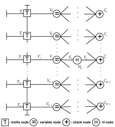
Figure 2: Normal graph of a NB-LDPC coded ISI channel.

Assume that the detector and the decoder are implemented with algorithms A and B, respectively. We define the following two different schedules

• $\mathbf{A\rightarrow B}$: The detector executes the algorithm $\mathbf{A}$ only once, then the decoder performs the decoding algorithm $\mathbf{B}$.

• $\mathbf{A\leftrightarrow B}$: The detector and the decoder work in an iterative manner by exchanging either soft messages or hard messages between A and B.

In this paper, a reduced complexity detection/decoding algorithm based on the max-log-MAP algorithm and $X$-EMS algorithms is proposed (max-log-MAP$\rightarrow$$X$-EMS or max-log-MAP$\leftrightarrow$$X$-EMS). For majority-logic decodable NB-LDPC codes, we propose a further reduced complexity detection/decoding algorithm based on the Viterbi algorithm and the GMLGD algorithm (Viterbi$\leftrightarrow$GMLGD). The conventional dectection/decoding algorithms based on the BCJR algorithm and the QSPA, denoted by BCJR$\rightarrow$QSPA and BCJR$\leftrightarrow$QSPA, will be taken as benchmarks for comparison.

Figure 3: Trellis representations of the dicode channel. (a) The original trellis. (b) The sectionalized trellis matched to $\mathbb{F}_{16}$.

II-D Sectionalized Trellis

It has been shown that the ISI channel can be represented by a time-invariant trellis [14]. At each stage, the trellis has $2^{L}$ states. Emitting from each state, there are two branches, corresponding to binary inputs 0 and 1, respectively. For convenience, this trellis is referred to as the original trellis. When an iterative joint decection/decoding algorithm is adopted, we need to exchange messages between the detector and the decoder. The processing of the decoder is symbol-oriented, while the original trellis is bit-oriented. So it is necessary to transform from symbol-based messages to bit-based messages and vice versa, which requires additional computational loads and may cause performance degradations. A way to avoid such a transformation is to work on a $sectionalized$ trellis [40] directly, which can be obtained from the original trellis. For example, the original trellis and the sectionalized trellis matched to $\mathbb{F}_{16}$ on the the dicode channel $f(D)=1-D$ are illustrated in the Fig. 3.

• The sectionalized trellis has $N$ section, which are indexed by $0\leq j\leq N-1$. The $j$-th section corresponds to the $j$-th coded symbol $v_{j}$.

• At each stage, there are $2^{L}$ states, which are simply indexed by $0\leq s\leq 2^{L}-1$. Each state at the $j$-th stage corresponds to a bipolar sequence of the length $L$, that is $s_{j}\leftrightarrow(x_{(j-1)L},\cdots,x_{jL-1})$, where $x_{t}$ is the input to the channel at time $t$, and ${x_{t},t<0}$ is assumed to be known at the receiver. The collection of the states at the $j$-th stage is denoted by $\mathcal{S}_{j}$.

• Emitting from each state, there are $2^{m}$ branches. Each branch in the $j$-th section is specified by a 4-tuple $\underline{b}\triangleq(s_{j},v_{j},{z}_{j},s_{j+1})$, where $v_{j}\in\mathbb{F}_{q}$ is the $j$-th possible coded symbol that takes the state from $s_{j}$ into $s_{j+1}$ and results in the noiseless output vector ${z}_{j}$ of length $m$. In other words, each branch in the sectionalized trellis corresponds to a path of length $m$ in the original trellis. The collection of branches in the $j$-th section is denoted by $\mathcal{B}_{j}$, we have $|\mathcal{B}_{j}|=2^{L+m}$.

II-E Possibility function Calculation

Like most reduced complexity algorithms, we use log-domain messages in the proposed algorithm. Let $Z$ be a discrete random variable taking on values over $\mathcal{Z}$. We use $P_{Z}(z),z\in\mathcal{Z}$ to denote its probability mass function (pmf). Its $possibility$ $function$ is defined as $L_{Z}(z)=[a_{0}\log P_{Z}(z)+a_{1}],z\in\mathcal{Z}$, where $[x]$ represents the integer closest to $x\in\mathbb{R}$ and $a_{0}>0,a_{1}\in\mathbb{R}$ are two constants. Obviously, we can confine the range of $L_{Z}(z)$ to be $[0,2^{p}-1]$ by properly choosing parameters $a_{0}$ and $a_{1}$. In this case $L_{Z}(z)$ is also referred to as a $p$-bit possibility function. The possibility function can be considered as an integer measure on the possibility of the occurrence of each value $z\in\mathcal{Z}$. Let $X$ denote the variable on the edge connecting the node $\mathcal{A}_{1}$ and $\mathcal{A}_{2}$ in Fig. 2. We will use $L_{X}^{(\mathcal{A}_{1}\rightarrow\mathcal{A}_{2})}$ to denote the message from $\mathcal{A}_{1}$ to $\mathcal{A}_{2}$.

To each branch in the $j$-th section of the sectionalized trellis, we assign an integer $L_{Z_{j}}^{(\mid\rightarrow\mathcal{T}_{j})}(z_{j})$, where $z_{j}$ is the associated noiseless output. The possibility function $L_{Z_{j}}^{(\mid\rightarrow\mathcal{T}_{j})}(z_{j})$ can be determined using the following algorithm.
Algorithm 1: Given the received vector $\underline{y}$, $2^{p}-1$ and the maximum allowable squared Euclidean distance $d_{max}$ for quantization. For $j=0,1,\cdots,N-1$,

Step 1

: Calculate $d(z_{t})=||y_{j}-z_{j}||^{2}$, which is the squared Euclidean distance between $y_{j}$ and $z_{j}$;

Step 2

: If $d(z_{t})>d_{max}$, set $d(z_{t})=d_{max}$;

Step 3

: For each noiseless output $z_{j}$, calculate

$$L_{Z_{j}}^{(\mid\rightarrow\mathcal{T}_{j})}(z_{j})=\left[\frac{d_{max}-d(z_{j})}{d_{max}}\times(2^{p}-1)\right].$$ (3)

It can be easily checked that $L_{Z_{j}}^{(\mid\rightarrow\mathcal{T}_{j})}(z_{j})$ is a $p$-bit possibility function. For the least possible element $z_{j}$, we have $L_{Z_{j}}^{(\mid\rightarrow\mathcal{T}_{j})}(z_{j})=0$; while for the most possible element $z_{j}$, we have $L_{Z_{j}}^{(\mid\rightarrow\mathcal{T}_{j})}(z_{j})\leq 2^{p}-1$. Notice that the variance of the noise is not required to determine $L_{Z_{j}}^{(\mid\rightarrow\mathcal{T}_{j})}(z_{j})$.

Remarks: It should be pointed out that the maximum allowable Euclidean distance $d_{max}$ is time-invariant which ensures that $a_{0}$ in the possibility function is time independent. In this paper, the max-log-MAP algorithm and the Viterbi algorithm are implemented over the sectionalized trellis with the $p$-bit possibility function as branch metrics. As a result, the detectors require only integer operations.

III The Max-log-MAP$\leftrightarrow$$X$-EMS Algorithm

III-A T-node: Max-log-MAP Detection

To each branch $b_{j}=(s_{j},v_{j},z_{j},s_{j+1})$ and $0\leq j<N$, we assign an integer metric

$$L_{j}(b_{j})=L_{Z_{j}}^{(\mid\rightarrow\mathcal{T}_{j})}(z_{j})+L_{V_{j}}^{(\mathcal{V}_{j}\rightarrow\mathcal{T}_{j})}(v_{j}),$$ (4)

where $L_{V_{j}}^{(\mathcal{V}_{j}\rightarrow\mathcal{T}_{j})}(v_{j})$ are initialized as zeros and $L_{Z_{j}}^{(\mid\rightarrow\mathcal{T}_{j})}(z_{j})$ is determined by Algorithm 1. Then we can execute the max-log-MAP algorithm to obtain an extrinsic possibility vector $L_{V_{j}}^{(\mathcal{T}_{j}\rightarrow\mathcal{V}_{j})}$, for $0\leq j\leq N-1$.

Remark: It should be pointed out that the possibility vector $L_{V_{j}}^{(\mathcal{T}_{j}\rightarrow\mathcal{V}_{j})}(v_{j})$ is normalized such that the reliability of the least possible element is equal to 0.

III-B V-node: Computing the Extrinsic Message to H-node

Given $X_{ij}=x$ , the event of an V-node $\mathcal{V}_{j}$ being satisfied is equivalent to the event $\{V_{j}=x\}\bigcap_{k\neq i}\{X_{ki}=x\}$. We have

$$L_{X_{ij}}^{(\mathcal{V}_{j}\rightarrow\mathcal{H}_{ij})}(x)=L_{V_{j}}^{(\mathcal{T}_{j}\rightarrow\mathcal{V}_{j})}(x)+\sum_{k\neq i}L_{X_{kj}}^{(\mathcal{H}_{kj}\rightarrow\mathcal{V}_{j})}(x),$$ (5)

where $L_{V_{j}}^{(\mathcal{T}_{j}\rightarrow\mathcal{V}_{j})}(x)$ is the message from the max-log-MAP detector and $L_{X_{kj}}^{(\mathcal{H}_{kj}\rightarrow\mathcal{V}_{j})}(x)$ are initialized as zeros for $x\in\mathbb{F}_{q}$.

III-C H-node: Message Permutation

Given $Y_{ij}=y$, the event of an H-node $\mathcal{H}_{ij}$ being satisfied is equivalent to the event $\{X_{ij}=h_{ij}^{-1}y\}$. We have

$$L_{Y_{ij}}^{(\mathcal{H}_{ij}\rightarrow\mathcal{C}_{i})}(y)=L_{X_{ij}}^{(\mathcal{V}_{j}\rightarrow\mathcal{H}_{ij})}(h_{ij}^{-1}y),\,y\in\mathbb{F}_{q}.$$ (6)

III-D C-node: Computing the Extrinsic Message to H-node

Message-truncation rules: Given the message $L_{Y_{ij}}^{(\mathcal{H}_{ij}\rightarrow\mathcal{C}_{i})}$, we can partition the finite field $\mathbb{F}_{q}$ into $\mathcal{F}$ and $\mathbb{F}_{q}-\mathcal{F}$. Three different message-truncation rules have been proposed in [7]. That are

$$\mathcal{F}_{M} = \{y\in\mathbb{F}_{q}|L_{Y_{ij}}^{(\mathcal{H}_{ij}\rightarrow\mathcal{C}_{i})}(y)\text{\rm~{}is one of the }M\text{~{}largest components of }L_{Y_{ij}}^{(\mathcal{H}_{ij}\rightarrow\mathcal{C}_{i})}\},$$

$$\mathcal{F}_{T}=\{y\in\mathbb{F}_{q}|L_{Y_{ij}}^{(\mathcal{H}_{ij}\rightarrow\mathcal{C}_{i})}(y)\geq T\},$$

and

$$\mathcal{F}_{D}=\{y\in\mathbb{F}_{q}|L_{max}-L_{Y_{ij}}^{(\mathcal{H}_{ij}\rightarrow\mathcal{C}_{i})}(y)\leq D\},$$

where $L_{max}$ denotes the largest component of $L_{Y_{ij}}^{(\mathcal{H}_{ij}\rightarrow\mathcal{C}_{i})}$ and $D$ is a designated parameter. In this paper, we give a new truncation rule

$$\mathcal{F}_{\mu}\stackrel{{\scriptstyle\Delta}}{{=}}\{y\in\mathbb{F}_{q}|L_{Y_{ij}}^{(\mathcal{H}_{ij}\rightarrow\mathcal{C}_{i})}(y)\geq\mu\},$$

where $\mu$ is determined by

$$\mu=\frac{1}{q}\sum_{y\in\mathbb{F}_{q}}L_{Y_{ij}}^{(\mathcal{H}_{ij}\rightarrow\mathcal{C}_{i})}(y)-c,$$ (7)

where $c$ is a constant to be designated. That is, $\mu$ is equal to the mean of the possibility vector $L_{Y_{ij}}^{(\mathcal{H}_{ij}\rightarrow\mathcal{C}_{i})}$ with an offset of $c$. The resultant EMS algorithm is referred to as $\mu$-EMS here.

Given a truncation rule, the possibility vector $L_{Y_{ij}}^{(\mathcal{C}_{i}\rightarrow\mathcal{H}_{ij})}$ from the C-node $\mathcal{C}_{j}$ to the H-node $\mathcal{H}_{ij}$ can be calculated by a reduced trellis search algorithm. See [7] for details.

Remark: The truncation rule $\mathcal{F}_{\mu}$ is simpler than the truncation rule $\mathcal{F}_{M}$, since no ordering is required. The truncation rule $\mathcal{F}_{\mu}$ is similar to $\mathcal{F}_{T}$ except that the threshold of $\mathcal{F}_{\mu}$ is data-dependent and hence can be matched to data and iterations.

III-E H-node: Message Permutation

Given $X_{ij}=x$, the event of an H-node $\mathcal{H}_{ij}$ being satisfied is equivalent to the event $\{Y_{ij}=h_{ij}x\}$. Then

$$L_{X_{ij}}^{(\mathcal{H}_{ij}\rightarrow\mathcal{V}_{j})}(x)=L_{Y_{ij}}^{(\mathcal{C}_{i}\rightarrow\mathcal{H}_{ij})}(h_{ij}x),\,x\in\mathbb{F}_{q}.$$ (8)

III-F V-node: Making Decisions and Computing the Extrinsic Message to T-node

For the V-node $\mathcal{V}_{j}$, $0\leq j\leq N-1$, calculate the message

$$L_{V_{j}}(x)=L_{V_{j}}^{(\mathcal{T}_{j}\rightarrow\mathcal{V}_{j})}(x)+\sum_{i\in\mathcal{M}_{j}}L_{X_{ij}}^{(\mathcal{H}_{ij}\rightarrow\mathcal{V}_{j})}(x)$$ (9)

and make decisions according to

$$\hat{v}_{j}=\arg\max_{x\in\mathbb{F}_{q}}L_{V_{j}}(x).$$ (10)

If $H\hat{\underline{v}}^{T}=\underline{0}$, output $\hat{\underline{v}}$ as the estimated codeword. If $H\hat{\underline{v}}^{T}\neq\underline{0}$, calculate the message $L_{V_{j}}^{(\mathcal{V}_{j}\rightarrow\mathcal{T}_{j})}$ from V-node $\mathcal{V}_{j}$ to T-node $\mathcal{T}_{j}$ as

$$L_{V_{j}}^{(\mathcal{V}_{j}\rightarrow\mathcal{T}_{j})}(x)=L_{V_{j}}(x)-L_{V_{j}}^{(\mathcal{T}_{j}\rightarrow\mathcal{V}_{j})}(x),$$ (11)

for $x\in\mathbb{F}_{q}$.

III-G Summary of The Max-log-MAP$\leftrightarrow$$X$-EMS Algorithm

• Initialization: Given $\underline{y}$ and a truncation rule $\mathcal{F}$, set a maximum iteration number $\mathcal{L}$ and an iteration variable $l=0$. For all $\mathcal{V}_{j}$ and $x\in\mathbb{F}_{q}$, set $L_{V_{j}}^{(\mathcal{V}_{j}\rightarrow\mathcal{T}_{j})}(x)=0$, $L_{X_{ij}}^{(\mathcal{H}_{ij}\rightarrow\mathcal{V}_{j})}(x)=0$.

• Iteration: while $l<\mathcal{L}:$

  1. Detection at T-node: Executing the max-log-MAP algorithm with the branch metrics as defined in (4) to obtain the possibility vector $L_{V_{j}}^{(\mathcal{T}_{j}\rightarrow\mathcal{V}_{j})}$.

  2. Messages processing at V-node: for all V-nodes, calculate $L_{X_{ij}}^{(\mathcal{V}_{j}\rightarrow\mathcal{H}_{ij})}$ according to (5).

  3. Messages permutation at H-node: for all H-nodes, permute the messages $L_{Y_{ij}}^{(\mathcal{H}_{ij}\rightarrow\mathcal{C}_{i})}$ according to (6).

  4. Messages processing at C-node: for all C-nodes, calculate the messages $L_{Y_{ij}}^{(\mathcal{C}_{i}\rightarrow\mathcal{H}_{ij})}$ according to the truncation rule $\mathcal{F}$.

  5. Messages permutation at H-node: for all H-nodes, permute the messages $L_{X_{ij}}^{(\mathcal{H}_{ij}\rightarrow\mathcal{V}_{j})}$ according to (8).

  6. Messages processing at V-node: for all V-nodes, calculate the messages $L_{V_{j}}$ and find $\hat{v}_{j}$. If $H\underline{\hat{v}}^{T}=0$, output $\underline{\hat{v}}$ and exit the iteration; otherwise, calculate the messages $L_{V_{j}}^{(\mathcal{V}_{j}\rightarrow\mathcal{T}_{j})}$.

  7. Increment $l$ by one.

• Failure: If $l=\mathcal{L}$, report a decoding failure.

Remark: Note that the proposed algorithm requires only integer operations and finite field operations.

IV The Viterbi$\leftrightarrow$GMLGD Algorithm

For majority-logic decodable NB-LDPC coded ISI channels, we propose a further complexity-reduced joint detection/decoding algorithm based on the Viterbi algorithm and the GMLGD algorithm. The parity-check matrix of a majority-logic decodable NB-LDPC code [39] has the property that no two rows (or two columns) have more than one position where they both have nonzero-components. This guarantees that the Tanner graph of the code is free of cycle of length 4 and hence has girth of at least 6. In practice, majority-logic decodable NB-LDPC codes with redundant rows [41] are preferred.

IV-A T-node: Viterbi Detection

To each branch $b_{j}=(s_{j},v_{j},z_{j},s_{j+1})$ and $0\leq j<N$, we assign an integer metric

$$L_{j}(b_{j})=L_{Z_{j}}^{(\mid\rightarrow\mathcal{T}_{j})}(z_{j})+L_{V_{j}}^{(\mathcal{V}_{j}\rightarrow\mathcal{T}_{j})}(v_{j}),$$ (12)

where $L_{V_{j}}^{(\mathcal{V}_{j}\rightarrow\mathcal{T}_{j})}(v_{j})$ are initialized as zeros and $L_{Z_{j}}^{(\mid\rightarrow\mathcal{T}_{j})}(z_{j})$ is determined by Algorithm 1. Then we can run the Viterbi algorithm through the sectionalized trellis to find a path $\hat{b}_{0},\hat{b}_{1},\cdots,\hat{b}_{N-1}$ such that the path metric $\sum_{0\leq j\leq N-1}L_{j}(\hat{b}_{j})$ is maximized. The associated input sequence $\hat{v}$ is then passed to the variable nodes as the hard decisions.

IV-B V-node: Syndrome Computation

After receiving the hard-decision vector $\hat{v}$ from the T-node, we may calculate the syndrome

$$\underline{s}=\underline{\hat{v}}H^{T}=(s_{0},s_{1},\cdots,s_{m-1}).$$ (13)

If $\underline{s}=0$, output $\underline{\hat{v}}$ as the decoding result; otherwise, the variable nodes send the hard decision vector $\underline{\hat{v}}$ together with the syndrome vector $\underline{s}$ to the check nodes.

IV-C C-node: Extrinsic Estimation

The $i$-th check node sends back an extrinsic estimate to the $j$-th variable node, which is denoted by $\sigma_{i\rightarrow j}$ and can be determined by

$$\sigma_{i\rightarrow j}=-h^{-1}_{i,j}(\sum_{j^{\prime}\in\mathcal{N}_{i}\backslash j}h_{i,j^{\prime}}\hat{v}_{j^{\prime}})=-h^{-1}_{i,j}s_{j}-\hat{v}_{j},$$ (14)

where $i\in\mathcal{M}_{j}$ and all the operations are executed in $\mathbb{F}_{q}$.

IV-D V-node: Possibility Function Updates

Intuitively, for each variable node $\mathcal{V}_{j}$, the occurrence of each $\alpha\in\mathbb{F}_{q}$ in the received messages $\{\sigma_{i\rightarrow j},i\in\mathcal{M}_{j}\}$ from check nodes reflects its possibility. Therefore these votes can be used to update the possibility function by increasing $L_{V_{j}}^{(\mathcal{V}_{j}\rightarrow\mathcal{T}_{j})}(v_{j})$, $v_{j}\in\mathbb{F}_{q}$, according to the following rule:

$$L_{V_{j}}^{(\mathcal{V}_{j}\rightarrow\mathcal{T}_{j})}(\sigma_{i\rightarrow j})\leftarrow L_{V_{j}}^{(\mathcal{V}_{j}\rightarrow\mathcal{T}_{j})}(\sigma_{i\rightarrow j})+1,$$ (15)

for all $i\in\mathcal{M}_{j}$. In words, for a given $\alpha\in\mathbb{F}_{q}$, $L_{V_{j}}^{(\mathcal{V}_{j}\rightarrow\mathcal{T}_{j})}(\alpha)$ is a counter that accumulates, up to and inclusive of the current iteration, all the occurrences of $V_{j}=v_{j}$ in the extrinsic messages sent back from the adjacent check nodes.

IV-E Summary of The Viterbi$\leftrightarrow$GMLGD Algorithm

1. Initialization: Given $\underline{y}$, calculate the $p$-bit possibility functions according to Algorithm 1. Select a maximum iteration number $\mathcal{L}>0$ and set $l=0$. For all $\mathcal{V}_{j}$ and $v_{j}\in\mathbb{F}_{q}$, set $L_{V_{j}}^{(\mathcal{V}_{j}\rightarrow\mathcal{T}_{j})}(v_{j})=0$.

2. Iteration: While $l<\mathcal{L}$:

   1. Detection at T-node: determines the hard decision sequence $\underline{\hat{v}}$ by executing the Viterbi algorithm with branch metrics as defined in (12).

   2. Syndrome computation at V-node: compute the syndrome $\underline{s}$ according to (13). If $\underline{s}=0$, output $\underline{\hat{v}}$ and exit the iteration; otherwise, send $\underline{s}$ and $\underline{\hat{v}}$ to the C-nodes.

   3. Extrinsic estimation at C-node: compute $\sigma_{i\rightarrow j}$ according to (14) and send them to the V-nodes.

   4. Possibility function update at V-node: update the possibility functions $L_{V_{j}}^{(\mathcal{V}_{j}\rightarrow\mathcal{T}_{j})}$ according to (15).

   5. Increment $l$ by one;

3. Failure Report: If $l=\mathcal{L}$, report a decoding failure.

V Complexity Analysis and The Numerical Results

V-A Complexity Analysis

The computational complexities per iteration of the Viterbi algorithm, the BCJR algorithm, the max-log-MAP algorithm, the GMLGD algorithm and the QSPA algorithm are shown in Table I, where $\delta$ denotes the number of non-zero elements in $\mathbf{H}$. However, the complexity of the $X$-EMS algorithm varies from iteration to iteration.

Apparently, for each iteration, the max-log-MAP$\leftrightarrow$$X$-EMS algorithm and the Viterbi$\leftrightarrow$GMLGD algorithm require less operations than BCJR$\leftrightarrow$QSPA. However, they may require more iterations to converge. Therefore, for a fair comparison, we take

$$\frac{\textrm{total number of operations of a given algorithm }}{\textrm{total number of operations of the BCJR$\leftrightarrow$QSPA algorithm }}$$ (16)

as the complexity measurement. Note that the statistical mean (averaging over frames) of the total number of operations involved in all iterations for decoding one frame is used in (16). Also note that the ratio in (16) only give a rough comparison, as different algorithms require different operations.

TABLE I: Computational Complexities of Different Algorithms Required Per Iteration.

	Detection algorithm			Decoding algorithm
	BCJR	Max-log-MAP	Viterbi	QSPA	GMLGD
Integer Addition		$4Nq2^{L}$	$N2^{L}$		$\delta+Nq2^{L}$
Integer Comparison		$3Nq2^{L}$	$Nq2^{L}$
Field Operation				$q\delta$	$4q\delta$
Real Multiplication	$4Nq2^{L}$			$2q\delta$
Real Addition	$3Nq2^{L}$			$2q^{2}\delta$
Real Division				$2q\delta$

V-B Numerical Results

Let $X_{s}$ and $X_{b}$ denote the parameters in the truncation rule $X$ for state metrics and branch metrics, respectively.

Example 1: Consider the dicode channel with characteristic polynomial $f(D)=1-D$. The simulated code is the 32-ary LDPC code $\mathcal{C}_{32}[961,765]$ of rate 0.79, which is constructed by the properties of finite fields [11]. The corresponding parity-check matrix has row weight $30$ and column weights $10$ and $11$. The squared Euclidean distances in Algorithm 1 are quantized with $p=9$ and $d_{max}=80$. All the algorithms are carried out with maximum iteration $\mathcal{L}=50$. The parameters of the max-log-MAP$\leftrightarrow$$X$-EMS algorithms are listed in the following:

1. for the $\mu$-EMS algorithm, $\mu$ is calculated by (7) with $c=1$; for the $D$-EMS algorithm, $D_{s}=50$, $D_{b}=40$; for the $T$-EMS algorithm, $T_{s}=20$, $T_{b}=10$; for $M$-EMS algorithm, $M=16$;

2. the scaling factors of the $M$-EMS algorithm, the $T$-EMS algorithm, the $D$-EMS algorithm and the $\mu$-EMS algorithm are $0.4$, $0.4$, $0.3$ and $0.4$, respectively.

The simulation results are shown in the Fig. 4. It can be seen that at bit error rate (BER) $10^{-5}$

1. the max-log-MAP$\leftrightarrow$$X$-EMS algorithms perform as well as the BCJR$\leftrightarrow$QSPA;

2. the max-log-MAP$\rightarrow$$X$-EMS algorithms have almost the same performances and suffer from performance degradations about 0.1 dB compared with BCJR$\leftrightarrow$QSPA;

3. the Viterbi$\leftrightarrow$GMLGD algorithm suffers from performance degradations about 0.6 dB compared with BCJR$\leftrightarrow$QSPA.

The complexity ratios of different detection/decoding algorithms are shown in Fig. 5. It can be seen that, at BER=$10^{-5}$, the Viterbi$\leftrightarrow$GMLGD algorithm is the simplest one with complexity ratio about 0.05, the max-log-MAP$\leftrightarrow$$\mu$-EMS and the max-log-MAP$\leftrightarrow$D-EMS have almost the same complexity with complexity ratio 0.5. We also notice that both max-log-MAP$\leftrightarrow$$T$-EMS algorithm and BCJR$\rightarrow$QSPA are more complex than BCJR$\leftrightarrow$QSPA. This is because the complexity reduction per iteration of these two algorithms is not enough to counteract the complexity increase caused by the extra iterations. In particular, $T$-EMS algorithm with a fixed performance-guaranteed threshold $T$ can not reduce too much computations at each iteration due to the large dynamic range of the messages. This motivated us to propose the $\mu$-EMS algorithm, which is similar to the $T$-EMS algorithm but with a dynamic and message-matched threshold.

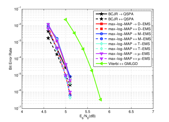
Figure 4: Error performances of different detection/decoding algorithms for decoding the $\mathcal{C}_{32}[961,765]$ coded dicode channel.

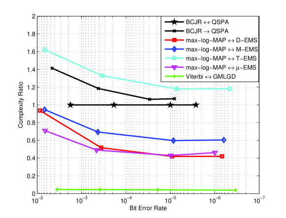
Figure 5: Complexity ratios of different detection/decoding algorithms for decoding the $\mathcal{C}_{32}[961,765]$ coded dicode channel.

Example 2: Consider an EPR4 channel with characteristic polynomial $f(D)=1+D-D^{2}-D^{3}$. The simulated code is a 16-ary NB-LDPC code $\mathcal{C}_{16}[225,173]$ of rate 0.77, which is constructed by the properties of finite fields [11]. The corresponding parity-check matrix has row weight $14$ and column weights $3$ and $4$. The squared Euclidean distances in Algorithm 1 are quantized with $p=9$ and $d_{max}=180$. All the algorithms are carried out with maximum iteration $\mathcal{L}=50$. The parameters for simulation are listed in the following:

1. for the $\mu$-EMS algorithm, $\mu$ calculated by (7) with $c=0$; for the $D$-EMS algorithm, $D_{s}=45$, $D_{b}=35$; for the $T$-EMS algorithm, $T_{s}=30$, $T_{b}=10$; for $M$-EMS algorithm, $M=10$;

2. the scaling factors of the $M$-EMS algorithm, the $T$-EMS algorithm, the $D$-EMS algorithm and the $\mu$-EMS algorithm are $0.6$, $0.6$, $0.6$ and $0.75$, respectively.

The simulation results are shown in the Fig. 6. It can be seen that at BER=$10^{-5}$

1. the max-log-MAP$\leftrightarrow$$X$-EMS algorithms perform as well as the BCJR$\leftrightarrow$QSPA;

2. the max-log-MAP$\rightarrow$$X$-EMS algorithms perform as well as the BCJR$\rightarrow$QSPA;

3. the max-log-MAP$\leftrightarrow$$X$-EMS algorithms perform about 0.4 dB better than BCJR$\rightarrow$QSPA.

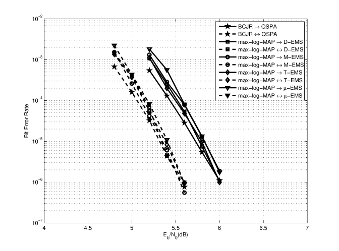
Figure 6: Error performances of different detection/decoding algorithms for decoding the $\mathcal{C}_{16}[225,173]$ coded EPR4 channel.

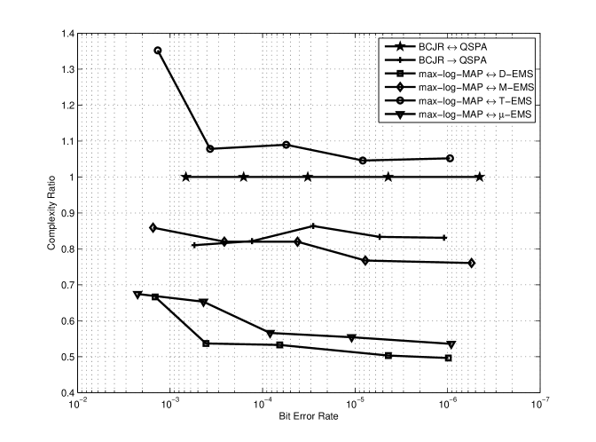
Figure 7: Complexity ratios of different detection/decoding algorithms for decoding the $\mathcal{C}_{16}[225,173]$ coded EPR4 channel.

The complexity ratios of different detection/decoding algorithms are shown in Fig. 7. It can be seen that, at BER=$10^{-5}$, the max-log-MAP$\leftrightarrow$D-EMS algorithm is the simplest one with complexity ratio about 0.5, the max-log-MAP$\leftrightarrow$$\mu$-EMS algorithm has a complexity with complexity ratio about 0.55.

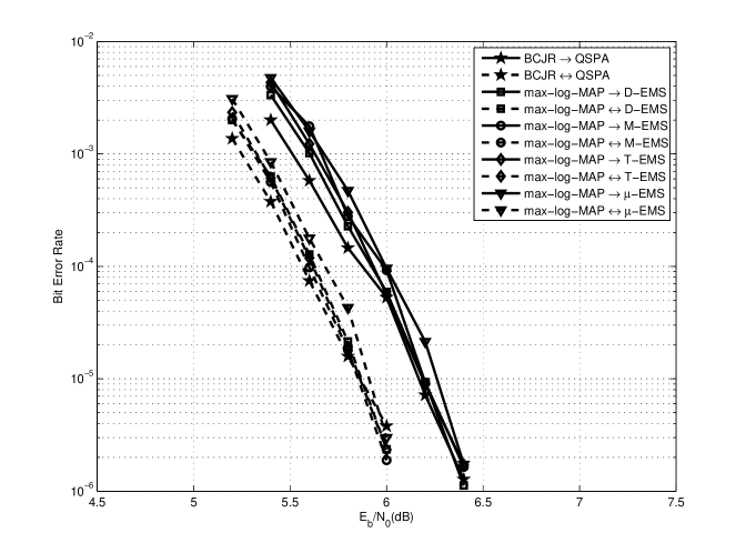
Figure 8: Error performances of different detection/decoding algorithms for decoding the $\mathcal{C}_{16}[225,173]$ coded Proakis. (b) channel.

Example 3: Consider the Proakis. (b) channel [13, Sec 9.4-3] with characteristic polynomial $f(D)=0.407+0.815D+0.407D^{2}$. The simulated code is a 16-ary NB-LDPC code $\mathcal{C}_{16}[225,173]$ of rate 0.77, which is constructed by the properties of finite fields. The corresponding parity-check matrix has row weight $14$ and column weights $3$ and $4$. The squared Euclidean distances in Algorithm 1 are quantized with $p=9$ and $d_{max}=60$. All the algorithms are carried out with maximum iteration $\mathcal{L}=50$. The parameters for simulation are listed in the following:

1. for the $\mu$-EMS algorithm, $\mu$ calculated by (7) with $c=0$; for the $D$-EMS algorithm, $D_{s}=45$, $D_{b}=35$; for the $T$-EMS algorithm, $T_{s}=10$, $T_{b}=5$; for $M$-EMS algorithm, $M=10$;

2. the scaling factors of the $M$-EMS algorithm, the $T$-EMS algorithm, the $D$-EMS algorithm and the $\mu$-EMS algorithm are $0.7$, $0.6$, $0.6$ and $0.75$, respectively.

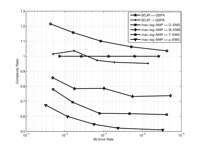
Figure 9: Complexity ratios of different detection/decoding algorithms for decoding the $\mathcal{C}_{16}[225,173]$ coded Proakis. (b) channel.

The simulation results are shown in the the Fig. 8. It can be seen that at BER=$10^{-5}$

1. the max-log-MAP$\leftrightarrow$$X$-EMS algorithms perform as well as the BCJR$\leftrightarrow$QSPA;

2. the max-log-MAP$\rightarrow$$X$-EMS algorithms perform as well as the BCJR$\rightarrow$QSPA;

3. the max-log-MAP$\leftrightarrow$$X$-EMS algorithms perform about 0.3 dB better than BCJR$\rightarrow$QSPA.

The complexity ratios of different detection/decoding algorithms are shown in Fig. 9. It can be seen that, at BER=$10^{-5}$, the max-log-MAP$\leftrightarrow$$\mu$-EMS algorithm is the simplest one with complexity ratio about 0.5.

Remark: From the preceding examples, it can be seen that the complexity ratio of max-log-MAP$\leftrightarrow$$\mu$-EMS algorithm is always around 0.5.

VI Conclusion

In this paper, we have proposed two low-complexity joint iterative detection/decoding algorithms for NB-LDPC coded ISI channels. The proposed algorithms work iteratively by exchanging either soft or hard messages between the detectors and the decoders. We have also presented a low-complexity decoding algorithm NB-LDPC codes. Simulation results show that the max-log-MAP$\leftrightarrow$$X$-EMS algorithm performs as well as BCJR$\leftrightarrow$QSPA, and the Viterbi$\leftrightarrow$GMLGD algorithm, which is the simplest one, suffers from a performance degradation within one dB compared with BCJR$\leftrightarrow$QSPA. These algorithms provide good candidates for trade-offs between performance and complexity.

Appendix A

A rough comparison between binary and NB-LDPC codes coded ISI channel is conducted in this appendix. We have simulated a binary LDPC code $\mathcal{C}_{2}[495,433]$ [42] and a 16-ary NB-LDPC code $\mathcal{C}_{16}[124,107]$. These two codes have almost the same bit lengths and code rates. The nonbinary code $\mathcal{C}_{16}[124,107]$ is constructed by the PEG algorithm [10] with column wight 2. We have simulated these two codes over EPR4 channels. The simulation results are shown in Fig. 10. It can be seen that $\mathcal{C}_{16}[124,107]$ performs about 0.6 dB better than $\mathcal{C}_{2}[495,433]$. We have also simulated these two codes over AWGN channels. The simulation results are also given in Fig. 10. It can be seen that $\mathcal{C}_{16}[124,107]$ performs only 0.2 dB better than $\mathcal{C}_{2}[495,433]$ as apposed to 0.6 dB. We conclude that NB-LDPC codes may be more suitable to combat inter-symbol interferences.

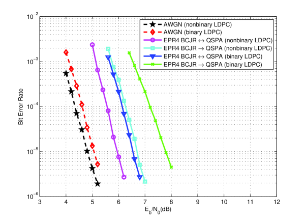
Figure 10: Error performances of different algorithms for decoding the $\mathcal{C}_{16}[124,107]$ and binary LDPC code (62,495) coded AWGN channel and the EPR4 channel.

References

- [1] R. G. Gallager, Low-Density Parity-Check Codes. Cambridge, MA: MIT Press, 1963.
- [2] M. Davey and D. MacKay, “Low-density parity check codes over GF(q),” IEEE Commun Lett., pp. 165 –167, 1998.
- [3] D. MacKay and M. Davey, “Evaluation of gallager codes for short block length and high rate applications,” in Proc. IMA Workshop Codes, Syst., Graphical Models, 1999.
- [4] L. Barnault and D. Declercq, “Fast decoding algorithm for LDPC over GF(),” in Proceeding of ITW2003, (Paris, France), pp. 70 –73, March/April 2003.
- [5] D. Declercq and M. Fossorier, “Decoding algorithms for nonbinary LDPC codes over GF(q),” IEEE Trans. Commun., vol. 55, pp. 633 –643, April 2007.
- [6] A. Voicila, D. Declercq, F. Verdier, M. Fossorier, and P. Urard, “Low-complexity decoding for non-binary LDPC codes in high order fields,” IEEE Trans. Commun., vol. 58, pp. 1365 –1375, May 2010.
- [7] X. Ma, K. Zhang, H. Chen, and B. Bai, “Low complexity X-EMS algorithms for nonbinary LDPC codes,” IEEE Trans. Commun., vol. 60, pp. 9 –13, Jan. 2012.
- [8] X. Wang, B. Bai, and X. Ma, “A low-complexity joint detection-decoding algorithm for nonbinary LDPC-coded modulation systems,” in Proc. IEEE Int. Symp. Inform. Theory, (Austin, Texas), pp. 794 –798, June 13-18 2010.
- [9] D. Zhao, X. Ma, C. Chen, and B. Bai, “A low complexity decoding algorithm for majority-logic decodable nonbinary LDPC codes,” Communications Letters, IEEE, vol. 14, pp. 1062 –1064, Nov. 2010.
- [10] X.-Y. Hu, E. Eleftheriou, and D. Arnold, “Regular and irregular progressive edge-growth Tanner graphs,” IEEE Trans. Inform. Theory, vol. 51, pp. 386–398, Jan. 2005.
- [11] L. Zeng, L. Lan, Y. Tai, S. Song, S. Lin, and K. Abdel-Ghaffar, “Constructions of nonbinary quasi-cyclic ldpc codes: A finite field approach,” IEEE Trans. Commun., vol. 56, pp. 545 –554, April 2008.
- [12] X. Jiang and M. H. Lee, “Large girth non-binary LDPC codes based on finite fields and euclidean geometries,” IEEE Signal Processing Letters, vol. 16, pp. 521 –524, June 2009.
- [13] J. G. Proakis and M. Salehi, Digital Communications. 5th ed. New York: McGraw-Hill, 2008.
- [14] G. D. Forney Jr., “Maximum-likelihood sequence estimation of digital sequences in the presence of intersymbol interference,” IEEE Trans. Inform. Theory, vol. 18, pp. 363 –378, March 1972.
- [15] G. D. Forney Jr., “The viterbi algorithm,” Proceedings of the IEEE, vol. 61, pp. 268 –278, March 1973.
- [16] L. R. Bahl, J. Cocke, F. Jelinek, and J. Raviv, “Optimal decoding of linear codes for minimizing symbol error rate,” IEEE Trans. Inform. Theory, vol. 20, pp. 284 –287, March 1974.
- [17] R. Kohno, S. Pasupathy, H. Imai, and M. Hatori, “Combination of cancelling intersymbol interference and decoding of error-correcting code,” IEE Proceedings F Communications, Radar and Signal Processing, vol. 133, pp. 224 –231, June 1986.
- [18] S. Prasad and S. Pathak, “Optimum data receivers for low SNR data signals in non-Gaussian noise and intersymbol interference: receiver structures and their performance analysis,” IEE Proceedings F Radar and Signal Processing, vol. 135, pp. 471 – 480, Oct. 1988.
- [19] J. Douillard, M. Jezequel, C. Berrou, A. Picart, P. Didier, and A. Glavieux, “Iterative correction of intersymbol interference: Turbo-equalization,” Eoropean Trans. Commun., vol. 6, pp. 507 –511, Sept. 1995.
- [20] D. Sebald and J. Bucklew, “A binary adaptive decision-selection equalizer for channels with nonlinear intersymbol interference,” IEEE Trans. Signal Processing, vol. 50, pp. 2286 – 2294, Sept. 2002.
- [21] T. Cheng, B. Belzer, and K. Sivakumar, “Row-column soft-decision feedback algorithm for two-dimensional intersymbol interference,” IEEE Signal Processing Letters, vol. 14, pp. 433 –436, July 2007.
- [22] R.-H. Peng, R.-R. Chen, and B. Farhang-Boroujeny, “Markov chain Monte Carlo detectors for channels with intersymbol interference,” IEEE Trans. Signal Processing, vol. 58, pp. 2206 –2217, April 2010.
- [23] L. Salamanca, J. Murillo-Fuentes, and F. Perez-Cruz, “Bayesian equalization for LDPC channel decoding,” IEEE Trans. Signal Processing, vol. 60, pp. 2672 –2676, May 2012.
- [24] C. Berrou, A. Glavieux, and P. Thitimajshima, “Near shannon limit error-correcting coding and decoding: Turbo-codes,” in Proc. IEEE Int. Conf. on Communications, (Geneva, Switzerland), pp. 1064 –1070, May 1993.
- [25] M. Tüchler, R. Kötter, and A. Singer, “Turbo equalization: principles and new results,” IEEE Trans. Inform. Theory, vol. 48, pp. 754 –767, May 2002.
- [26] J. Gunther, M. Ankapura, and T. Moon, “A generalized LDPC decoder for blind turbo equalization,” IEEE Trans. Signal Processing, vol. 53, pp. 3847 – 3856, Oct. 2005.
- [27] B. M. Kurkoski, P. H. Siegel, and J. K. Wolf, “Joint message-passing decoding of LDPC codes and partial-response channels,” IEEE Trans. Inform. Theory, vol. 48, pp. 1410 –1422, June 2002.
- [28] H. Yang and W. E. Ryan, “Low-floor detection/decoding of LDPC-coded partial response channels,” IEEE Journal on Selected Areas in Communications, vol. 28, pp. 252 –260, Feb. 2010.
- [29] W. Ryan, “Performance of high-rate turbo codes on PR4-equalized magnetic recording channels,” in in Proc. IEEE Int. Conf. on Communications, (Atlanta, GA), pp. 947 –951, June 1998.
- [30] T. V. Souviginer, M. Öberg, P. H. Siegel, R. E. Swanson, and J. K. Wolf, “Turbo decoding for partial response channels,” IEEE Trans. Commun., vol. 48, pp. 1297 –1308, Aug. 2000.
- [31] H. Song and V. Kumar, “Low-density parity check codes for partial response channels,” IEEE Signal Processing Magazine, vol. 21, pp. 56 – 66, Jan. 2004.
- [32] A. Kavčic̀, X. Ma, and M. Mitzenmacher, “Binary intersymbol interference channels: Gallager codes, density evolution and code performance bounds,” IEEE Trans. Inform. Theory, vol. 49, pp. 1636 –1652, July 2003.
- [33] G. Colavolpe and G. Germi, “On the application of factor graphs and the sum-product algorithm to ISI channels,” IEEE Trans. Commun., vol. 53, pp. 818 –825, May 2005.
- [34] F. R. Kschischang, B. J. Frey, and H. A. Loeliger, “Factor graphs and the sum-product algorithm,” IEEE Trans. Inform. Theory, vol. 47, pp. 498 –519, Feb. 2001.
- [35] G. D. Forney Jr., “Codes on graphs: Normal realizations,” IIEEE Trans. Inform. Theory, vol. 47, pp. 520 –548, Feb. 2001.
- [36] X. Ma and A. Kavčić, “Path partitions and forward-only trellis algorithms,” IEEE Trans. Inform. Theory, vol. 49, pp. 38–52, March 2003.
- [37] P. Robertson, E. Villebrun, and P. Hoeher, “A comparison of optimal and sub-optimal MAP decoding algorithms operating in the log domain,” in Proc. ICC 95, (Seattle, WA), pp. 1009 –1013, June 1995.
- [38] M. Fossorier, F. Burkert, S. Lin, and J. Hagenauer, “On the equivalence between SOVA and max-log-MAP decodings,” IEEE Commun. Lett., vol. 2, pp. 137 –139, May 1998.
- [39] S. Lin and D. J. Costello, Error Control Coding: Fundamentals and Applications. 2nd ed. Englewood Cliffs NJ: Prentice-Hall, 2004.
- [40] A. Lafourcade and A. Vardy, “Optimal sectionalization of a trellis,” IEEE Trans. Inform. Theory, vol. 42, pp. 689 –703, May 1996.
- [41] Q. Huang, K. Liu, and Z. Wang, “Low-density arrays of circulant matrices: Rank and row-redundancy, and QC-LDPC codes,” in 2012 IEEE International Symposium on Information Theory, pp. 3073 –3077, 2012.
- [42] D. MacKay. Encyclopedia of Sparse Graph Codes. [Online]. Available: http://wol.ra.phy.cam.ac.uk/mackay/codes/data.html.