Lensing and Dynamics in Two Simple Steps

Abstract

We present a ready-to-use method to constrain the density distribution in early-type galaxy lenses. Assuming a power-law density profile, then joint use of the virial theorem and the lens equation yields simple formulae for the power-law index (or logarithmic density gradient). Any dependence on orbital anisotropy can be tightly constrained or even erased completely. Our results rely just on surface brightnesses and line-of-sight kinematics, making deprojection unnecessary. We revisit three systems that have already been examined in the literature (the Cosmic Horseshoe, the Jackpot and B1608+656) and provide our estimates. Finally, we show that the method yields a good approximation for the density profile even when the true profile is a broken power-law, albeit with a mild bias towards isothermality.

1 Introduction

When a galaxy acts as a gravitational lens, its mass can be probed independently via analyses of lensing properties and stellar kinematics. This combination has proved a powerful way of breaking both the mass-sheet degeneracy in lensing and the mass-anisotropy degeneracy in dynamics. It was first tackled by combining the lens equation with the Jeans equations (cf Treu & Koopmans, 2004), usually with the assumption of a constant velocity anisotropy profile. Of course, Jeans analyses give no guarantee that the chosen models correspond to physically consistent distribution functions (cf An & Evans, 2009; Ciotti & Morganti, 2010). Latterly, sophisticated methods to build distribution functions of lensing galaxies using the Schwarzschild method have been developed (e.g. Barnabè & Koopmans, 2007). In both cases, though, observational data are often not enough to constrain all of the parameters used.

Here, we provide a simple method for combining lensing and dynamics. Our starting point is the virial theorem, which has the significant advantage that no assumption as to the anisotropy profile is ever needed. As a concrete case, we examine the scale-free density profiles $\rho\propto r^{-\gamma}$. Given an accurate photometric profile and an estimate of the Einstein radius from strong lensing, our method straightforwardly yields the value of the logarithmic gradient of the density $\gamma$. It does not require any photometric deprojection and it is robust under changes in orbital structure of the lens galaxy. By considering three benchmark lenses – the Cosmic Horseshoe, the Jackpot and B1608+656 – we demonstrate that our method performs very creditably against more sophisticated algorithms. Given its simplicity, we believe it provides the natural first step in combining lensing and dynamics.

2 The Virial Theorem and the Lens Equation

One global constraint for galaxy lenses is given by the projected mass within the Einstein radius. Another is given by the virial theorem, which links the average kinematics of stars to the total mass density and luminosity. In other words, lensing probes projected masses, while photometry and line-of-sight motions together trace the three-dimensional potential, so a combined analysis allows us to infer properties of the total mass profile. Here, we will quantify this framework by exploiting only the direct observables: surface brightnesses and projected kinematics.

2.1 A Global Constraint

The basic observables are the Einstein ring radius ${R_{\rm E}}$, the surface brightness profile of the lens galaxy $\Sigma(R)$, together with the mean $\overline{v}_{\rm los}(R)$ and mean-square velocities $\overline{v^{2}}_{\rm los}(R)$ of stars along the line of sight at projected radius $R$.

Let us start with the lens equation. For a spherical lens, this gives the projected mass within the Einstein ring radius as

$$M_{\rm p}({R_{\rm E}})=\pi{\Sigma_{\rm cr}}{R_{\rm E}}^{2},$$ (1)

where ${\Sigma_{\rm cr}}$ is the critical surface density (see e.g., Schneider, Ehlers & Falco, 1992) For a power-law lens with an assumed total (i.e., luminous and dark matter) density $\rho=\rho_{0}(r/r_{0})^{-\gamma}$, the projected mass within the Einstein ring $M_{\rm p}({R_{\rm E}})$ reduces to a standard integral which can be done analytically. This yields:

$$\rho_{0}r_{0}^{\gamma}=(1-\kappa){\Sigma_{\rm cr}}{R_{\rm E}}^{\gamma-1}\frac{(3-\gamma)\Gamma(\gamma/2)}{2\sqrt{\pi}\Gamma((\gamma-1)/2)}\ ,$$ (2)

where we have allowed for the presence of an external mean convergence $\kappa$ inside the Einstein radius (e.g., Suyu et al, 2010). The external shear, even if important in modelling the lens, does not enter the mass normalization.

The second ingredient is the virial theorem. For a spherical system, the virial theorem can be formulated in terms of the surface brightness as (Agnello & Evans, 2012)

$$\langle\overline{v^{2}}_{\rm los}\rangle_{L}=\frac{16\pi G}{3L_{\rm T}}\int_{0}^{\infty}\Sigma(R)R\int_{0}^{R}\frac{\rho(r)r^{2}}{\sqrt{R^{2}-r^{2}}}\mathrm{d}r\mathrm{d}R$$ (3)

Here, $L_{\rm T}$ is the total luminosity, and we have introduced the notation

$$\langle\mathcal{A}\rangle_{L}\equiv{2\pi\over L_{\rm T}}\int_{0}^{\infty}{\mathcal{A}\Sigma(R)R}\mathrm{d}R.$$ (4)

to denote luminosity averages.

For power-law density profiles, eqs (2) and (3) give us immediately

$$\frac{\langle\overline{v^{2}}_{\rm los}\rangle_{L}}{c^{2}}\frac{D_{l}D_{ls}}{D_{s}R_{E}}=\frac{1-\kappa}{3\pi}\mathcal{F}(\gamma)\frac{\langle R^{2-\gamma}\rangle_{L}}{R_{E}^{2-\gamma}}\ .$$ (5)

Here $D_{\rm s},$ $D_{\rm l}$ and $D_{\rm ls}$ are the angular-diameter distances to the source, to the lens and from lens to source respectively. The function $\mathcal{F}$ is analytic, namely

$$\mathcal{F}(x)=\frac{\Gamma(x/2)\Gamma((5-x)/2)}{\Gamma(2-x/2)\Gamma((x-1)/2)}\ .$$ (6)

It is worth pausing to examine eq (5), which is the first main result of this Letter. Every quantity is known, or can be computed directly from the observations, with the sole exception of $\gamma$. Hence, the power-law index $\gamma$ depends just on global, measurable quantities. There is no dependence whatsoever on the orbital anisotropy.

The magnitude of the external convergence $\kappa$ is affected by the mass-sheet degeneracy (Falco et al., 1985). Following the results of Suyu et al (2010), we adopt a prior distribution for $\kappa$ with zero mean and $\approx 0.05$ dispersion. This translates into a $\approx 5\%$ uncertainty in the mass-normalization, or $\approx 2.5\%$ in the velocity dispersion. The latter is small compared to the typical $\approx 15\%$ statistical uncertainties of present-day measurements.

Figure 1: Logarithm of the aperture correction $1/(1+\epsilon)$ as a function of $\gamma$. The lines are plotted for a de Vaucouleurs surface photometry and ${R_{\rm ap}}/{R_{\rm e}}=0.5,0.6,1,2,3,10.$ Smaller aperture radii correspond to steeper aperture corrections.

2.2 Aperture Corrections

In practice, the kinematics are measured inside a finite aperture radius ${R_{\rm ap}}$ and blurred by a point-spread function (PSF). Hence, we re-state the results in terms of the aperture-averaged line of sight motions, introducing an aperture-correction:

$$\langle\overline{v^{2}}_{\rm los}\rangle_{L}=\langle\overline{v^{2}}_{\rm los}\rangle_{L(<{R_{\rm ap}})}(1+\epsilon)\ .$$ (7)

The function $\epsilon$ characterises how the aperture-average is related to the luminosity-average over the whole system. If the kinematics are measured well beyond the effective radius, or if the latter is small compared to the fiber aperture, then the correction is small and $\epsilon\approx 0$. For lenses in the SLACS sample, ${R_{\rm ap}}$ is $\approx 3/5$ of the de Vaucouleurs effective radius ${R_{\rm e}}$ (cf Auger et al., 2010). Hence we need to inquire whether averaging within the aperture radius (rather than to infinity) introduces an effective dependence on orbital anisotropy. Let us assume, as a starting point, that the system is isotropic within the effective radius, as suggested by dynamical analyses of nearby elliptical galaxies (Saglia et al., 1993; Gerhard et al., 2001). We regard this as an informed prior on orbital structure and examine in a second step the consequences of anisotropy. We integrate the isotropic Jeans equations and reconstruct the kinematic profile to quantify how much of it is left out of the aperture-average. For a $\delta$-function PSF, the result can be stated explicitly in terms of the surface brightness, namely

$$1+\epsilon=\frac{L_{<{R_{\rm ap}}}}{L_{T}}\left(\frac{I(0,\gamma)}{I(0,\gamma)-I({R_{\rm ap}},\gamma)}\right)\ ,$$ (8)

were $L_{<{R_{\rm ap}}}$ is the luminosity from projected radii less than the aperture radius ${R_{\rm ap}}$. We have also defined

$$I(y,\gamma)=\int_{y}^{\infty}\Sigma(R)R^{3-\gamma}g(y/R,\gamma)\mathrm{d}R\ ,$$ (9)

where the kernel $g(y,\gamma)$ is given by

$$g(x,\gamma)=(4-\gamma)\int_{x}^{1}\sqrt{\frac{u^{2}-x^{2}}{1-u^{2}}}u^{3-\gamma}\mathrm{d}u$$

$$+(\gamma-1)x^{2}\int_{x}^{1}\sqrt{\frac{u^{2}-x^{2}}{1-u^{2}}}u^{1-\gamma}\mathrm{d}u\ .$$ (10)

Eq (8) is the second main result of this Letter. Here, the aperture correction is expressed as a double quadrature that depends on the power-law density exponent $\gamma$. Fig. 1 shows the aperture correction $1/(1+\epsilon)$ for a de Vaucouleurs profile with different values of ${R_{\rm ap}}/{R_{\rm e}}$. For lenses in the SLACS sample, $\gamma\approx 2$, so that the correction is generally steeper in $\gamma$ than the right-hand side of eq (5) and only weakly dependent on the details of photometry. This behaviour is understandable, since the additional requirement of pressure isotropy reduces the freedom in $\gamma$ to yield physically consistent solutions.

The aperture corrections also can be evaluated for anisotropic velocity dispersions, such as

$$\beta(r)=1-{\overline{v^{2}}_{\theta}\over\overline{v^{2}}_{r}}={\beta_{0}\frac{r^{2}}{r^{2}+r_{a}^{2}}}.$$ (11)

The systematic error on $\gamma$ given by neglecting anisotropy is limited in modulus to $\lesssim 5\%$ for the SLACS sample, when $\beta({R_{\rm e}})$ varies between -0.5 and 0.5 and a de Vaucouleurs luminous profile is used. The correction to $\epsilon$ is always negative for $\beta_{0}>0$ (radial anisotropy) and positive for $\beta_{0}<0$ (tangential anisotropy). This is an extension of the result found in Koopmans et al. (2009), where Hernquist or Jaffe luminous densities with uniform anisotropy were used to quantify the effect. We conclude that at least as far as aperture corrections are concerned, velocity anisotropy is a secondary effect.

2.3 Algorithm

Eqs (5) and (8) provide a prediction for the root-mean-square velocities along the line of sight, for which it is convenient to introduce the shorthand

$$v(\gamma)\doteq\sqrt{\langle\overline{v^{2}}_{\rm los}\rangle_{L}}.$$ (12)

On the other hand, observations give us a value and uncertainties for the same observable, say $\sigma\pm\delta\sigma$.

With larger fiber apertures, or extended long-slit measurements, there is no need to make any aperture corrections. So, for each value of $\gamma$, eq (5) yields the virial prediction and the likelihood on the density exponent is simply

$$p(\gamma)\propto\exp-{[v(\gamma)-\sigma]^{2}\over 2\delta\sigma^{2}}.$$ (13)

If the kinematics are not measured over a sufficiently wide radial range, then both sides of eq (5) are divided by the aperture correction $1+\epsilon$, as defined in eq (8), to get the new prediction for the line of sight velocity dispersions and the new likelihood for $\gamma$. This step is critical when the aperture is a small fraction of the effective radius, as $v(\gamma)$ may be very flat or even non-monotonic (Fig. 2); in this case, if the aperture correction is ignored then the inference on $\gamma$ may be biased and imprecise.

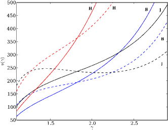
Figure 2: The relationship between the model power-law index $\gamma$ and the model velocity dispersion $v$ without aperture corrections (dashed) and including aperture corrections (solid) for the 3 example lenses discussed in Section 3 (red, labelled H): Horseshoe; black, labelled J: Jackpot; blue, labelled B: B1608). In addition to large quantitative changes in the predicted dispersions, the aperture corrections also yield significant qualitative changes; in all cases the relationship gets steeper when the aperture correction is applied. This leads to more precise inference, particularly in the case of the Jackpot, where the flatness of the uncorrected relation implies little information on the slope given an observed dispersion, and the non-monotonic nature of $v(\gamma)$ also leads to a (biased) bi-modal inference.

As illustrated, the combination of lensing and dynamics has been reduced to the routine procedure of evaluating a single non-linear function. When the PSF has a non-negligible width, the aperture-averages are more representative of the luminosity averages. In that case, the aperture corrections are smaller than predicted by eq (8), which assumes a $\delta$-function PSF. The density exponent must then lie between the uncorrected and aperture-corrected estimates.

3 Examples

We first discuss three particular lens systems, comparing the performance of our method with results in the literature. The first quoted error bars from our method refer just to the statistical uncertainties propagated by line of sight kinematics. The sources of systematic error (anisotropy, external convergence and PSF) are briefly touched upon case by case and incorporated as a second uncertainty in the aperture-corrected estimates. We adopt as this systematic uncertainty $5\%$ of the mean value, even though this might be too pessimistic. Finally, we examine the consequences of applying our single power-law inference to broken power-law density profiles.

3.1 The Cosmic Horseshoe Lens (SDSS J1148+1930)

The Cosmic Horseshoe was discovered by Belokurov et al. (2007). It is a massive early-type lens at a redshift $z_{\rm l}=0.44$ surrounded by a loose group. The extended source galaxy at $z_{\rm s}=2.381$ (Dye et al., 2008) is lensed into a nearly complete Einstein ring. Early studies used estimates of the velocity dispersion derived from low resolution spectra.

Recently, Spiniello et al. (2011) used high resolution spectra derived from X-Shooter on the Very Large Telescope to provide line of sight kinematic profiles out to the effective radius. Using the Jeans equations, they find a logarithmic density slope of $\gamma=1.72^{+0.05}_{-0.06}$. We use their kinematic data ($\sigma=352\pm 19$ inside a circularised aperture of 0.84^′′) with a de Vaucouleurs luminous profile (with an effective radius of 1.96^′′; the Einstein radius is 5.1^′′), to get an estimated value of $\gamma=1.76\pm 0.08$ without aperture corrections and $1.80\pm 0.04\pm 0.09$ when aperture corrections are included. This is perfectly compatible with the Spiniello et al. (2011) estimate within the uncertainties. It is worth remarking that their Jeans analysis is fit to the line-of-sight velocity dispersion profile, neglecting any internal rotation. Our method exploits the whole velocity second moment $\langle\overline{v^{2}}_{\rm los}\rangle_{L}$, (i.e. pressure and rotation), which is slightly higher than the velocity dispersion alone. Moreover, we rely just on the surface brightness profile $\Sigma(R)$ instead of using an approximation for the deprojected density, which they are forced to do so as to employ the Jeans equations.

3.2 The Jackpot Lens (SDSSJ0946+1006)

The Jackpot Lens was discovered by Bolton et al. (2008) and subsequently analysed by Gavazzi et al. (2008). The system is unusual in that it possesses two Einstein rings, as two different high redshift sources are lensed by the same foreground elliptical galaxy at a redshift of $z_{\rm l}=0.22$.

With the photometric, kinematic, and lensing data provided by Auger et al. (2009) and Auger et al. (2010), our aperture-corrected power-law exponent is $\gamma=2.01\pm 0.15\pm 0.1$. This is perfectly consistent with the estimate $2.01\pm 0.18$ of Auger et al. (2010), where the uncertainties from the PSF are fully accounted for. Sonnenfeld et al. (2012) use a strong prior on $\gamma$ obtained by more detailed lensing analyses and information from both sources to find $\gamma=1.98\pm 0.03$, in good agreement with the previous estimates. Using their double Sersic photometry, our method yields $\gamma=2.06\pm 0.04\pm 0.1$ if we use the inner Einstein radius. On the other hand, their Jeans analysis approximates the luminous profile with two cored pseudo-Jaffe profiles, but it is not immediately clear how a flat-top luminous density can be supported self-consistently in a cusped potential like the scale-free ones, so the underlying dynamical model may be unphysical (An & Evans, 2009).

The value $\gamma=2.20\pm 0.03$ estimated by Vegetti et al. (2010) is obtained by examining a small region around the inner Einstein radius, whereas our method and the Jeans analysis in Sonnenfeld et al. (2012) provide an estimate of the global density exponent on the whole radial range out to the Einstein radii. This discrepancy hints that the true density profile is not a simple power-law. One possibility is that the analysis by Vegetti et al. (2010) probes the density profile where both baryons and dark matter are important, and the assumption of a single power-law is too facile.

3.3 B1608+656

B1608+656 (Myers et al., 1995; Snellen et al., 1995; Fassnacht et al., 1996) consists of an early-type galaxy lens with a small companion at $z_{\rm l}=0.63.$ The source is an active galaxy at $z_{\rm s}=1.394.$

In Koopmans et al. (2003), the lensing morphology and time delays of the images were used to constrain the lensing potential. This was subsequently refined by incorporating kinematic information in Suyu et al (2010), which allowed them to break the degeneracies between density slope and Hubble constant that would otherwise afflict the problem (Wucknitz, 2002). Their complete analysis, assuming Jaffe or Hernquist luminous densities, gives $\gamma=2.08\pm 0.03$. We use the same data as Suyu et al (2010) ($\sigma=260\pm 15$ in a 0.42^′′ aperture, the effective radius is 0.6^′′, and the Einstein radius of the main lens is 0.83^′′) to obtain $\gamma=2.39\pm 0.09$ for the uncorrected estimate and $\gamma=2.14\pm 0.06\pm 0.11$ including aperture corrections. As with the Horseshoe, this estimate is consistent with but slightly larger than previous estimates, although the Suyu et al (2010) result is mostly driven by the lensing information from the extended source structure that is ignored in our analysis.

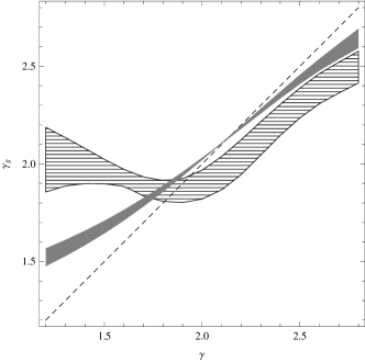
Figure 3: The globally-estimated density exponent $\gamma_{\rm g}$ versus the inner power-law exponent $\gamma$ of the broken power-law model, as given in eq (14). The dashed band illustrates the model prediction when the aperture is very large (between 0.25 and 1 times the scale radius of the broken power-law), while the grey band is for a small aperture that is 5 to 20 times smaller than the effective radius. The widths of the bands demonstrate the effects of changing the size of the effective radius of the luminous tracer for fixed aperture and scale radius; for large effective radii the steep outer halo is given more weight and $\gamma_{\rm g}$ is more discrepent from the true value $\gamma$.

3.4 Extensions

So far, we have assumed a power-law total density. Whether justifiable or not, this assumption is widely used out to length scales an order of magnitude greater than the effective radius $r_{\rm e}$ or Einstein radius ${R_{\rm E}}$ (cf Gavazzi et al., 2007; Humphrey & Buote, 2010). However, the normalisation from lensing is set by the projected mass within the (cylindrical) Einstein radius, which in turn includes mass at large (spherical polar) radii where the density profile may fall off differently from any inner power-law.

As an example, let us consider the broken power-law density distribution

$$\rho(r)=\frac{\rho_{0}(r/r_{\rm s})^{-\gamma}}{(1+r^{2}/r_{\rm s}^{2})^{(3-\gamma)/2}}\ .$$ (14)

This behaves like $\rho\propto r^{-\gamma}$ for $r<r_{\rm s}$, while $\rho\rightarrow r^{-3}$ for $r\gg r_{\rm s}$. The appearance of an explicit scale-radius $r_{\rm s}$ means that the lensing and virial equations are not enough to fix all the independent parameters. The virial constraint is then just another piece of information to be incorporated into the lensing decomposition, albeit now with more complicated kernels than in eqs  (5) and (8).

However, we may ask if approximating this profile with a global power-law $\rho=\rho_{1}(r/r_{1})^{-\gamma_{\rm g}}$ gives a reasonable representation of the inner parts of the system. The virial estimates can help us answer this question. In particular, we find the global power-law index $\gamma_{\rm g}$ by fixing ${R_{\rm E}}$ and $\langle\overline{v^{2}}_{\rm los}\rangle_{L<R_{\rm ap}}$ to the ones given by the double-power law profile of eq (14).

Figure 3 shows bands of solutions corresponding to the physically plausible range of halo scale lengths with $5\leq r_{\rm s}/{R_{\rm E}}\leq 20$. The dashed curve represents situations when the aperture is large (here, 5 times the Einstein radius, or 0.25 to 1 times the scale radius). It is clear that for such large apertures the power-law approximation for the density profile is inadequate, with the central slope being grossly over-estimated for small values of $\gamma$ and systematically under-estimated for large values of gamma. This trend persists when the aperture is small (the grey curve, where the aperture is equal to the effective radius, i.e., 5 to 20 times smaller than the scale radius) but with a significantly smaller bias.

The bias of the estimator $\gamma_{\rm g}$ is always towards isothermality and in the case of small apertures (e.g., consistent with the apertures used for observations) the bias tends to favour $\gamma_{\rm g}\approx 2.1$. This is remarkably close to the mean power-law index inferred for the SLACS lenses (Koopmans et al., 2009; Auger et al., 2010; Barnabè et al., 2011), although power-law indices inferred without the use of dynamics yield similar results (e.g., Dobke & King, 2006). Nevertheless, the magnitude of the bias is also smallest at $\gamma_{\rm g}\approx 2.1$ and suggests that the power-law index estimates from lensing and dynamics robustly describe the central density profile even if the true mass density distribution is a broken power-law.

4 Conclusions

We have presented a simple method to combine strong lensing and stellar dynamics without any need of prescribing the poorly known velocity dispersion anisotropy. Using measurements of the Einstein ring radius, the photometric profile and the global kinematics, we have shown how to obtain the logarithmic slope of the density $\gamma$. When the kinematics are measured on a small aperture, then the density slope $\gamma$ and the velocity anisotropy $\beta$ are intertwined, but procedures have been developed to characterise the influence of anisotropy robustly. Above all, our algorithm has the significant advantage of simplicity – all that is needed is the numerical solution of a single non-linear equation to obtain an estimate for the density slope $\gamma$. We have verified that our algorithm works well by comparison with analyses in the literature for three well-studied lenses.

The set of hypotheses used here is common to a majority of Jeans equation analyses, but the lack of any need for marginalisation over velocity anisotropy $\beta$ in our method allows us to separate the statistical uncertainties from systematics. Also, our formulae require only a profile for the surface brightness, avoiding any additional uncertainty from deprojection inherent in applications of the Jeans equations.

Why does our simple method work so well? A major reason is that velocity anisotropy is never significant at the centres of early-type galaxies. If the kinematics are known within a finite aperture radius, then anisotropy can affect our result. However, this correction is always small, and isotropic models give a good guide as to its magnitude. The fact that the virial theorem is independent of the velocity anisotropy enables us to sidestep difficulties that Jeans or phase-space modelling must necessarily confront.

The main limitation that this method shares with Jeans analysis is observational: aperture-averaged line of sight motions must be suitably dealt with to account for different possible sources of bias. However, when care is taken in assessing these effects, our procedure gives the density slope $\gamma$ in terms of directly observable quantities and can be used as a robust and quick method of carrying out lensing plus dynamics decompositions.

AA thanks the Science and Technology Facility Council and the Isaac Newton Trust for the award of a studentship. We wish to thank Nicola C. Amorisco, Iulia T. Simion and Vasily Belokurov for significant feedback on the manuscript, as well as Alessandro Sonnenfeld for discussing some details of his analysis with us. The anonymous referee gave useful comments that helped us improve the paper.

References

- Agnello & Evans (2012) Agnello, A. & Evans, N.W. 2012, ApJL, 754, L39
- An & Evans (2009) An, J. H., & Evans, N.W. 2009, ApJ, 701, 1500
- Auger et al. (2009) Auger, M. W., Treu, T., Bolton, A. S., et al. 2009, ApJ, 705, 1099
- Auger et al. (2010) Auger, M. W., Treu, T., Bolton, A. S., et al. 2010, ApJ, 724, 511
- Barnabè & Koopmans (2007) Barnabè, M., & Koopmans, L. V. E. 2007, ApJ, 666, 726
- Barnabè et al. (2011) Barnabè, M., Czoske, O., Koopmans, L. V. E., Treu, T., & Bolton, A. S. 2011, MNRAS, 415, 2215
- Belokurov et al. (2007) Belokurov, V., Evans, N. W., Moiseev, A., et al. 2007, ApJL, 671, L9
- Bolton et al. (2008) Bolton, A. S., Burles, S., Koopmans, L. V. E., et al. 2008, ApJ, 682, 964
- Ciotti & Morganti (2010) Ciotti, L., & Morganti, L. 2010, MNRAS, 408, 1070
- Dobke & King (2006) Dobke, B. M., & King, L. J. 2006, AA, 460, 647
- Dye et al. (2008) Dye, S., Evans, N. W., Belokurov, V., Warren, S. J., & Hewett, P. 2008, MNRAS, 388, 384
- Falco et al. (1985) Falco, E. E., Gorenstein, M. V., & Shapiro, I. I. 1985, ApJL, 289, L1
- Fassnacht et al. (1996) Fassnacht, C. D., Womble, D. S., Neugebauer, G., et al. 1996, ApJL, 460, L103
- Gavazzi et al. (2007) Gavazzi, R., Treu, T., Rhodes, J. D., et al. 2007, ApJ, 667, 176
- Gavazzi et al. (2008) Gavazzi, R., Treu, T., Koopmans, L. V. E., et al. 2008, ApJ, 677, 1046
- Gerhard et al. (2001) Gerhard, O., Kronawitter, A., Saglia, R. P., & Bender, R. 2001, AJ, 121, 1936
- Humphrey & Buote (2010) Humphrey, P. J., & Buote, D. A. 2010, MNRAS, 403, 2143
- Koopmans et al. (2003) Koopmans, L. V. E., Treu, T., Fassnacht, C. D., Blandford, R. D., & Surpi, G. 2003, ApJ, 599, 70
- Koopmans et al. (2009) Koopmans, L. V. E., Bolton, A., Treu, T., et al. 2009, ApJL, 703, L51
- Myers et al. (1995) Myers, S. T., Fassnacht, C. D., Djorgovski, S. G., et al. 1995, ApJL, 447, L5
- Saglia et al. (1993) Saglia, R. P., Bertin, G., Bertola, F., et al. 1993, ApJ, 403, 567
- Schneider, Ehlers & Falco (1992) Schneider P., Ehlers J., Falco E.E., 1992, Gravitational Lenses, Springer Verlag, New York
- Snellen et al. (1995) Snellen, I. A. G., de Bruyn, A. G., Schilizzi, R. T., Miley, G. K., & Myers, S. T. 1995, ApJL, 447, L9
- Sonnenfeld et al. (2012) Sonnenfeld, A., Treu, T., Gavazzi, R., et al. 2012, ApJ, 752, 163
- Spiniello et al. (2011) Spiniello, C., Koopmans, L. V. E., Trager, S. C., Czoske, O., & Treu, T. 2011, MNRAS, 417, 3000
- Suyu et al (2010) Suyu, S. H., et al. 2010 ApJ, 711, 201
- Treu & Koopmans (2004) Treu, T., & Koopmans, L. V. E. 2004, ApJ, 611, 739
- Vegetti et al. (2010) Vegetti, S., Koopmans, L. V. E., Bolton, A., Treu, T., & Gavazzi, R. 2010, MNRAS, 408, 1969
- Wucknitz (2002) Wucknitz, O. 2002, MNRAS, 332, 951