Finite–$t$ and target mass corrections to deeply virtual Compton scattering

Abstract

We carry out the first complete calculation of kinematic power corrections $\sim t/Q^{2}$ and $\sim m^{2}/Q^{2}$ to the helicity amplitudes of deeply-virtual Compton scattering. This result removes an important source of uncertainties in the QCD predictions for intermediate momentum transfers $Q^{2}\sim 1-10$ GeV² that are accessible in the existing and planned experiments. In particular the finite–$t$ corrections are significant and must be taken into account in the data analysis.

Deeply Virtual Compton Scattering (DVCS) is the simplest process that gives access to generalized parton distributions (GPDs) and is receiving a lot of attention Diehl:2003ny ; Belitsky:2005qn . The existing experimental results come from HERMES and Jefferson Lab (Hall A and CLAS) and many more measurements are planned after the Jefferson Lab $12$ GeV upgrade and at COMPASS-II at CERN. Since the bulk of the existing and expected data is for photon virtualities $Q^{2}<5$ GeV², corrections of the type $m^{2}/Q^{2},\,\,t/Q^{2}$, where $m$ is the target (nucleon) mass and $t=(p^{\prime}-p)^{2}$ is the momentum transfer to the target, can have significant impact on the data analysis and should be taken into account. The finite–$t$ corrections are of particular importance if one wants to study the three-dimensional picture of the proton in longitudinal and transverse plane Burkardt:2002hr , in which case the $t$–dependence has to be measured in a sufficiently broad range.

The necessity of taking into account kinematic power corrections to DVCS is widely acknowledged Belitsky:2005qn ; Anikin:2000em ; Blumlein:2000cx ; Kivel:2000rb ; Radyushkin:2000ap ; Belitsky:2000vx ; Belitsky:2001hz ; Geyer:2004bx ; Blumlein:2006ia ; Blumlein:2008di ; Belitsky:2010jw . Early attempts to calculate such corrections by analogy to Nachtmann corrections Nachtmann:1973mr to the structure functions in deep-inelastic lepton-nucleon scattering produced results that were not gauge invariant and not translation invariant with respect to the choice of the positions of the electromagnetic currents. The reason is that in addition to Nachtmann-type contributions related to subtraction of traces in the leading-twist operators one must take into account their higher-twist descendants obtained by adding total derivatives: $\mathcal{O}_{1}\sim\partial^{2}\mathcal{O}_{\mu_{1}\ldots\mu_{n}}$, and $\mathcal{O}_{2}\sim\partial^{\mu_{1}}\mathcal{O}_{\mu_{1}\ldots\mu_{n}}$, where $\mathcal{O}_{\mu_{1}\ldots\mu_{n}}$ are the usual leading-twist operators. The problem arises because matrix elements of the operator $\mathcal{O}_{2}$ on free quarks vanish Ferrara:1972xq . Thus in order to find its leading-order coefficient function in the operator product expansion (OPE) of two electromagnetic currents one is forced to consider either more complicated (quark-antiquark-gluon) matrix elements, or stay with the quark-antiquark ones but go over to the next-to-leading order in $\alpha_{s}$. In both cases the real difficulty is not the calculation of the relevant Feynman diagrams, but the necessity to separate the contribution of interest from the “genuine” quark-gluon twist-four operators.

This problem was solved in Refs. Braun:2011zr ; Braun:2011dg using conformal symmetry which implies that coefficient functions of “kinematic” and “genuine” twist-four operators are mutually orthogonal with a proper weight function Braun:2009vc ; Braun:2012bg . Using this approach we have calculated in Ref. Braun:2012bg the finite–$t$ and target-mass corrections to DVCS for the study case of a scalar target. We verified gauge- and translation-invariance and, most importantly, found that the structure of kinematic corrections proves to be consistent with collinear factorization. In this letter we present our final results for the helicity amplitudes of DVCS to the $1/Q^{2}$ accuracy for the physically interesting case of the spin-1/2 (nucleon) target. This result removes one important source of uncertainties in the QCD predictions for intermediate photon virtualities that are accessible in the existing and planned experiments.

The DVCS amplitude $\gamma^{*}(q)+N(p)\to\gamma(q^{\prime})+N(p^{\prime})$ is defined by the matrix element of the time-ordered product of two electromagnetic currents, sandwiched between the nucleon states

$$i\int\!d^{4}x\int\!d^{4}y\,e^{-iqx+iq^{\prime}y}\langle{p^{\prime}|T\{j^{\rm em}_{\mu}(x)j^{\rm em}_{\nu}(y)\}|p}\rangle=$$ (1)

$$= (2\pi)^{4}\delta(p+q-p^{\prime}-q^{\prime})\,\mathcal{A}_{\mu\nu}(q,q^{\prime},p)\,.$$

Introducing the photon polarization vectors $(\varepsilon^{\pm,0}q)=0$, $(\varepsilon^{\pm}q^{\prime})=0$ one can write $\mathcal{A}_{\mu\nu}$ in terms of helicity amplitudes

$$\!\mathcal{A}_{\mu\nu}= \,\,\varepsilon^{+}_{\mu}\varepsilon^{-}_{\nu}\mathcal{A}^{++}+\varepsilon^{-}_{\mu}\varepsilon^{+}_{\nu}\mathcal{A}^{--}+\varepsilon^{0}_{\mu}\varepsilon^{-}_{\nu}\mathcal{A}^{0+}$$

$$+\varepsilon^{0}_{\mu}\varepsilon^{+}_{\nu}\mathcal{A}^{0-}\!+\!\varepsilon^{+}_{\mu}\varepsilon^{+}_{\nu}\mathcal{A}^{+-}\!+\!\varepsilon^{-}_{\mu}\varepsilon^{-}_{\nu}\mathcal{A}^{-+}\!+\!q^{\prime}_{\nu}\mathcal{A}_{\mu}^{(3)}\!.$$ (2)

The last term $\sim q^{\prime}_{\nu}$ is of no interest as it does not contribute to any observable.

The helicity-conserving amplitudes are the leading ones in the scaling limit, $A^{\pm\pm}\sim\mathcal{O}(Q^{0})$, and the helicity-flip amplitudes are power-suppressed: $A^{0\pm}\sim\mathcal{O}(Q^{-1})$, $A^{\pm\mp}\sim\mathcal{O}(Q^{-2})$. Thus in order to calculate physical observables to the $1/Q^{2}$ accuracy one has to take into account $1/Q^{2}$ corrections to $A^{++}$ and $A^{--}$, whereas for the helicity-flip amplitudes the leading power accuracy is sufficient.

The definition of helicity amplitudes depends on a reference frame. We use the photon momenta, $q$ and $q^{\prime}$, to define a longitudinal plane spanned by the two light-like vectors

$$n=q^{\prime}\,,\qquad\tilde{n}=-q+(1-\tau)\,q^{\prime}\,,$$ (3)

where $\tau=t/(Q^{2}+t)$, $Q^{2}=-q^{2}$. For this choice the momentum transfer to the target $\Delta=p^{\prime}-p=q-q^{\prime}$, $t=\Delta^{2}$ is purely longitudinal and the target (proton) momenta have a nonzero transverse component

$$|P_{\perp}|^{2}=-m^{2}-\frac{t}{4}\frac{1-\xi^{2}}{\xi^{2}}\sim\mathcal{O}(Q^{0})\,,$$ (4)

where $P=(p+p^{\prime})/2$ and the skewedness parameter is defined as $\xi=-(\Delta\cdot q^{\prime})/(2(P\cdot q^{\prime}))$ .

The condition $|P_{\perp}|^{2}>0$ translates to the lower bound $|t|>|t_{\rm min}|=4m^{2}\xi^{2}/(1-\xi^{2})$, cf. Belitsky:2005qn .

We choose the polarization vectors as follows Braun:2012bg

$$\varepsilon^{0}_{\mu}= -\left(q_{\mu}-q^{\prime}_{\mu}{q^{2}}/{(qq^{\prime})}\right)/{\sqrt{-q^{2}}}\,,$$

$$\varepsilon^{\pm}_{\mu}= (P^{\perp}_{\mu}\pm i\bar{P}^{\perp}_{\mu})/\sqrt{2}\,,$$ (5)

where $P^{\perp}_{\mu}=g_{\mu\nu}^{\perp}P^{\nu}$, $\bar{P}^{\perp}_{\mu}=\epsilon_{\mu\nu}^{\perp}P^{\nu}$ and

$$g_{\mu\nu}^{\perp}= g_{\mu\nu}-(q_{\mu}q^{\prime}_{\nu}+q^{\prime}_{\mu}q_{\nu})/(qq^{\prime})+{q^{\prime}_{\mu}}q^{\prime}_{\nu}\,{q^{2}}/(qq^{\prime})^{2}\,,$$

$$\epsilon_{\mu\nu}^{\perp}= \epsilon_{\mu\nu\alpha\beta}{q^{\alpha}q^{\prime\beta}}/(qq^{\prime})\,.$$ (6)

Each helicity amplitude involves the sum over quark flavors, $\mathcal{A}=\sum e_{q}^{2}\mathcal{A}_{q}$, where $e_{q}$ is the quark electromagnetic charge, and is written in terms of the leading-twist GPDs $H^{q},E^{q},\widetilde{H}^{q},\widetilde{E}^{q}$. For the GPD definitions we follow Ref. Diehl:2003ny .

The calculation is similar to the case of the scalar target considered in Ref. Braun:2012bg so that in this letter we only present the final expressions. Note that the electromagnetic gauge invariance is guaranteed to twist-four accuracy already on the operator level and is embedded in the definition of helicity amplitudes. The translation invariance (independence on the shift of the positions of the electromagnetic currents in Eq. (1): $x\to x+\delta,y\to y+\delta$) is nontrivial and provides a strong check of the calculation, see Ref. Braun:2012bg . The results can conveniently be written in terms of the vector and axial-vector bispinors

$$v^{\mu}=\bar{u}(p^{\prime})\gamma^{\mu}u(p)\,, a^{\mu}=\bar{u}(p^{\prime})\gamma^{\mu}\gamma_{5}u(p)\,.$$ (7)

We define $v_{\perp}^{\pm}=(v\cdot\varepsilon^{\pm})\,,\quad a_{\perp}^{\pm}=(a\cdot\varepsilon^{\pm})\,,\quad P_{\perp}^{\pm}=(P\cdot\varepsilon^{\pm})\,.$ Although $P_{\perp}^{+}=P_{\perp}^{-}=|P_{\perp}|/\sqrt{2}$ we prefer this notation to keep trace of the polarization vectors. We also use a shorthand notation

$$X^{q}(x,\xi,t)=H^{q}(x,\xi,t)+E^{q}(x,\xi,t)\,$$ (8)

and rewrite the helicity-conserving amplitudes in terms of the vector- and axial-vector invariant functions as

$$\frac{1}{2}(\mathcal{A}_{q}^{++}\!+\!\mathcal{A}_{q}^{--})= \frac{(vP)}{2m^{2}}\,\mathbb{V}^{q}_{1}+\frac{(vq^{\prime})}{(qq^{\prime})}\,\mathbb{V}^{q}_{2}\,,$$ (9)

$$\frac{1}{2}(\mathcal{A}_{q}^{++}\!-\!\mathcal{A}_{q}^{--})= \frac{(a\Delta)}{4m^{2}}\,\mathbb{A}^{q}_{1}+\frac{(aq^{\prime})}{(qq^{\prime})}\,\mathbb{A}^{q}_{2}\,.$$ (10)

The following expressions for $\mathbb{V}^{q}_{k}$, $\mathbb{A}^{q}_{k}$ present our main result:

$$\mathbb{V}^{q}_{1}= \Big{(}1-\frac{t}{2Q^{2}}\Big{)}E^{q}\otimes{C}_{0}^{-}+\frac{t}{Q^{2}}E^{q}\otimes\mathcal{C}_{1}^{-}-\frac{2}{Q^{2}}\Big{(}\frac{t}{\xi}+2|P_{\perp}|^{2}\xi^{2}\partial_{\xi}\Big{)}\xi^{2}\partial_{\xi}E^{q}\otimes{C}_{2}^{-}+\frac{8m^{2}}{Q^{2}}\xi^{2}\partial_{\xi}\xi\,X^{q}\otimes{C}_{2}^{-}\,,$$ (11a)

$$\mathbb{V}^{q}_{2}= \Big{(}1-\frac{t}{2Q^{2}}\Big{)}\xi\,X^{q}\otimes{C}_{0}^{-}+\frac{t}{Q^{2}}\xi\,X^{q}\otimes\mathcal{C}_{1}^{-}-\frac{4}{Q^{2}}\biggl{[}\Big{(}|P_{\perp}|^{2}\xi^{2}\partial_{\xi}+\frac{t}{\xi}\Big{)}\xi^{2}\partial_{\xi}-\frac{t}{2}\biggr{]}\xi\,X^{q}\otimes{C}_{2}^{-}\,,$$ (11b)

$$\mathbb{A}^{q}_{1}= \Big{(}1-\frac{t}{2Q^{2}}\Big{)}\xi\,\widetilde{E}^{q}\otimes{C}_{0}^{+}+\frac{t}{Q^{2}}\xi\,\widetilde{E}^{q}\otimes{C}_{1}^{+}-\frac{2}{Q^{2}}\Big{(}\frac{t}{\xi}+2|P_{\perp}|^{2}\xi^{2}\partial_{\xi}\Big{)}\xi^{2}\partial_{\xi}\xi\,\widetilde{E}^{q}\otimes{C}_{2}^{+}+\frac{8m^{2}}{Q^{2}}\xi^{2}\partial_{\xi}\widetilde{H}^{q}\otimes{C}_{2}^{+}\,,$$ (11c)

$$\mathbb{A}^{q}_{2}= \Big{(}1-\frac{t}{2Q^{2}}\Big{)}\xi\,\widetilde{H}^{q}\otimes{C}_{0}^{+}+\frac{t}{Q^{2}}\xi\,\widetilde{H}^{q}\otimes{C}_{1}^{+}-\frac{4}{Q^{2}}\biggl{[}\Big{(}|P_{\perp}|^{2}\xi^{2}\partial_{\xi}+\frac{t}{\xi}\Big{)}\xi^{2}\partial_{\xi}-\frac{t}{2}\biggr{]}\xi\,\widetilde{H}^{q}\otimes{C}_{2}^{+}\,.$$ (11d)

In addition, for the helicity-flip amplitudes we obtain

$$\mathcal{A}_{q}^{0,\pm}= \frac{2}{Q}\biggl{\{}\left(v_{\perp}^{\pm}-4P_{\perp}^{\pm}\frac{(vq^{\prime})}{Q^{2}}\xi^{2}\partial_{\xi}\right)\xi\,X^{q}\otimes{C}_{1}^{-}$$

$$\hskip 14.22636pt\pm\left(a_{\perp}^{\pm}-4P_{\perp}^{\pm}\frac{(aq^{\prime})}{Q^{2}}\xi^{2}\partial_{\xi}\right)\xi\,\widetilde{H}^{q}\otimes{C}^{+}_{1}$$

$$\hskip 14.22636pt+P_{\perp}^{\pm}\frac{(vP)}{m^{2}}\xi^{2}\partial_{\xi}\,E^{q}\otimes{C}_{1}^{-}$$

$$\hskip 14.22636pt\pm P_{\perp}^{\pm}\frac{(a\Delta)}{2m^{2}}\xi^{2}\partial_{\xi}\,\xi\,\widetilde{E}^{q}\otimes{C}_{1}^{+}\biggr{\}}$$ (12)

and

$$\mathcal{A}_{q}^{\mp\pm}= -\frac{8P_{\perp}^{\pm}}{Q^{2}}\biggl{\{}\Big{(}v_{\perp}^{\pm}-2P_{\perp}^{\pm}\frac{(vq^{\prime})}{Q^{2}}\,\xi^{2}\partial_{\xi}\Big{)}\xi^{2}\partial_{\xi}\,X^{q}\otimes{[x{C}_{1}^{-}]}$$

$$\hskip 14.22636pt\pm\Big{(}a_{\perp}^{\pm}-2P_{\perp}^{\pm}\frac{(aq^{\prime})}{Q^{2}}\xi^{2}\partial_{\xi}\Big{)}\xi^{2}\partial_{\xi}\,\xi\,\widetilde{H}^{q}\otimes{C}_{1}^{+}$$

$$\hskip 14.22636pt+P_{\perp}^{\pm}\frac{(vP)}{2m^{2}}\xi^{3}\partial_{\xi}^{2}\,E^{q}\otimes{[xC_{1}^{-}]}$$

$$\hskip 14.22636pt\mp P_{\perp}^{\pm}\frac{(a\Delta)}{4m^{2}}\xi^{3}\partial_{\xi}^{2}\xi^{2}\widetilde{E}^{q}\otimes{C}_{1}^{+}\biggr{\}}.$$ (13)

In all cases $\partial_{\xi}=\partial/\partial\xi$ and the notation $F\otimes C$ stands for the convolution of a GPD $F$ with a coefficient function $C$:

$$F\otimes C\equiv\int dx\,F(x,\xi,t)\,C(x,\xi)\,.$$

The coefficient functions ${C}_{k}^{\pm}(x,\xi)$ are given by the following expressions:

$${C}_{0}^{\pm}(x,\xi)= \frac{1}{\xi+x-i\epsilon}\pm\frac{1}{\xi-x-i\epsilon}\,,$$

$${C}^{\pm}_{1}(x,\xi)= \frac{1}{x-\xi}\ln\Big{(}\frac{\xi+x}{2\xi}-i\epsilon\Big{)}\pm(x\leftrightarrow-x)\,,$$

$${C}_{2}^{\pm}(x,\xi)= \biggl{\{}\frac{1}{\xi+x}\Big{[}\operatorname{Li}_{2}\Big{(}\frac{\xi-x}{2\xi}+i\epsilon\Big{)}-\operatorname{Li}_{2}(1)\Big{]}$$

$$\pm(x\leftrightarrow-x)\biggr{\}}+\frac{1}{2}{C}_{1}^{\pm}(x,\xi)\,.$$ (14)

Note that ${C}_{0}^{\pm}$ have simple poles at $x=\pm\xi$ whereas ${C}_{1,2}^{\pm}$ have a milder (logarithmic) singularity at the same points. This ensures that the kinematic power corrections are factorizable, at least to the leading order in $\alpha_{s}$. In the DVCS kinematics

$$(vq^{\prime})\sim(aq^{\prime})=\mathcal{O}(Q^{2})\,, (vP)\sim(a\Delta)=\mathcal{O}(Q^{0})$$ (15)

so that the helicity-conserving amplitudes (11a) – (11d) include leading contributions $\mathcal{O}(1/Q^{0})$ and the corrections $\mathcal{O}(1/Q^{2})$, whereas all terms in Eqs. (12) and (Finite–$t$ and target mass corrections to deeply virtual Compton scattering) are of the order $\mathcal{O}(1/Q)$ and $\mathcal{O}(1/Q^{2})$, respectively, as expected.

Our results for the DVCS helicity amplitudes have a similar structure to those in Ref. Braun:2012bg for the scalar target correction . The main difference is the appearance of a large target mass correction to the contribution of the GPD $E^{q}$ ($\widetilde{E}^{q}$) that involves $X^{q}$ ($\widetilde{H}^{q}$), cf. the last term in the first line of Eq. (11a) (Eq. (11c)).

It has become customary to parametrize the DVCS amplitude (2) in terms of the so-called Compton form factors (CFFs) $\mathcal{H}$ and $\mathcal{E}$ Belitsky:2005qn

$$\mathcal{A}_{\mu\nu}=-\frac{g_{\mu\nu}^{\perp}}{2(Pq^{\prime})}\left[(\bar{u}\not{q}^{\prime}u)\,\mathcal{H}+\frac{i}{2m}(\bar{u}\sigma^{\mu\nu}q^{\prime}_{\mu}\Delta_{\nu}u)\,\mathcal{E}\right]+\ldots$$ (16)

In our notation

$$\mathcal{H}=\mathbb{V}_{1}-{\mathbb{V}_{2}}/\xi\,, \mathcal{E}=-\mathbb{V}_{1}\,,$$ (17)

where $\mathbb{V}_{k}=\sum_{q}e^{2}_{q}\mathbb{V}^{q}_{k}$.

A detailed study of the numerical impact of the kinematic corrections on different DVCS observables goes beyond the tasks of this letter. For orientation, we have calculated the corrections to the imaginary parts of the CFFs $\mathcal{H}$ and $\mathcal{E}$ which involve the GPDs in the DGLAP region only. To this end we use the GPD model of Refs. Hyde:2011ke ; Guidal:2004nd :

$$\left\{\begin{matrix}H^{q}\\ E^{q}\end{matrix}\right\}(x,\xi,t)=\int d\beta\int d\alpha\,\delta(x-\beta-\xi\alpha)f_{q}(\beta,\alpha,t)\,,$$

where the double distribution $f_{q}$ is written as

$$f_{q}(\beta,\alpha,t)=h(\beta,\alpha)|\beta|^{-\alpha^{\prime}t}q(\beta)\left\{\begin{matrix}1\\ \kappa_{q}(1-\beta)^{\eta_{q}}/A_{q}\end{matrix}\right.\,.$$

Here $q(\beta)$ is the MRST2002 NNLO valence $u$- and $d$-quark distribution Martin:2002dr ) and the profile function $h$ is given by the following expression:

$$h(\beta,\alpha)=\frac{3}{4}{((1-|\beta|)^{2}-\alpha^{2}})/{(1-|\beta|)^{3}}\,,$$

where $k_{u}\simeq 1.7$ and $k_{d}\simeq-2.0$ are the anomalous magnetic moments, $\eta_{u}\simeq 1.7$ and $\eta_{d}\simeq 0.57$ Guidal:2004nd , and $A_{q}=\int d\beta\,(1-\beta)^{\eta_{q}}q(\beta)$.

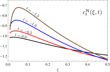
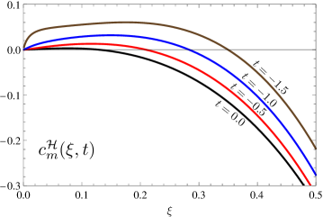
Figure 1: The coefficients $c_{t}^{\mathcal{H}}(\xi,t)$ (upper panel) and $c_{m}^{\mathcal{H}}(\xi,t)$ (lower panel) for different values of $t$ (in $\text{GeV}^{2}$).

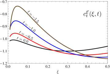
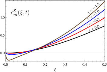
Figure 2: The coefficients $c_{t}^{\mathcal{E}}(\xi,t)$ (upper panel) and $c_{m}^{\mathcal{E}}(\xi,t)$ (lower panel) for different values of $t$ (in $\text{GeV}^{2}$).

We consider the following ratios

$$\frac{\text{Im}\mathcal{F}-\text{Im}\mathcal{F}^{LO}}{\text{Im}\mathcal{F}^{LO}}=\frac{t}{Q^{2}}c_{t}^{\mathcal{F}}(\xi,t)+\frac{m^{2}}{Q^{2}}c_{m}^{\mathcal{F}}(\xi,t)\,,$$ (18)

where $\mathcal{F}=\{\mathcal{H},\mathcal{E}\}$,

$$\text{Im}\,\mathcal{H}^{LO}= \pi\sum_{q}e^{2}_{q}\big{[}H^{q}(-\xi,\xi,t)-H^{q}(\xi,\xi,t)\big{]}\,,$$ (19)

and similar for $\text{Im}\,\mathcal{E}^{LO}$. The coefficients $c_{t}^{\mathcal{F}}(\xi,t)$ depend on $t$ because of the non-factorizable $t$-dependence of the GPDs through the Regge trajectory.

In Fig. 1 we show $c_{t}^{\mathcal{H}}(\xi,t)$ and $c_{m}^{\mathcal{H}}(\xi,t)$ as a function of $\xi$ for several $t$-values: $-t=0,0.5,1.0,1.5$ GeV². The same is shown in Fig. 2 for $c_{t}^{\mathcal{E}}(\xi,t)$ and $c_{m}^{\mathcal{E}}(\xi,t)$. One sees that the corrections to $\mathcal{E}$ are in general larger than for the $\mathcal{H}$ form factor; in particular $\mathcal{E}$ receives a relatively large proton mass correction.

Finally, note that the finite-$t$ correction depends on the definition of the skewedness parameter $\xi$, which is not unique. If one defines $\xi$ through the Bjorken $x_{B}$ parameter, $\xi_{B}=x_{B}/(2-x_{B})$, which seems to be natural from the experimental point of view (the relation of “our” $\xi$ to $\xi_{B}$ is given in Eq. ​(125) in Ref. Braun:2012bg ), $c_{t}^{\mathcal{H},\mathcal{E}}(\xi,t)$ change accordingly, but in general do not become smaller.

To summarize, in this work we have calculated, for the first time, the kinematic power corrections $\sim t/Q^{2}$ and $\sim m^{2}/Q^{2}$ to the helicity amplitudes of deeply virtual Compton scattering. These corrections are important for intermediate momentum transfers $Q^{2}\sim 1-10$ GeV² that are accessible in the existing and planned experiments, and have to be taken into account in the data analysis. In particular the finite–$t$ corrections are indispensable if one aims to study “holographic” images of the proton in the transverse plane, in which case the $t$-dependence must be measured in a broad range.

References

(1)
M. Diehl,
Phys. Rept. 388 (2003) 41.
(2)
A. V. Belitsky and A. V. Radyushkin,
Phys. Rept. 418, 1 (2005).
(3)
M. Burkardt,
Int. J. Mod. Phys. A 18 (2003) 173.
(4)
I. V. Anikin, B. Pire and O. V. Teryaev,
Phys. Rev. D 62 (2000) 071501.
(5)
J. Blumlein and D. Robaschik,
Nucl. Phys. B 581 (2000) 449.
(6)
N. Kivel, M. V. Polyakov, A. Schäfer and O. V. Teryaev,
Phys. Lett. B 497 (2001) 73.
(7)
A. V. Radyushkin and C. Weiss,
Phys. Rev. D63 (2001) 114012.
(8)
A. V. Belitsky and D. Mueller,
Nucl. Phys. B 589, 611 (2000).
(9)
A. V. Belitsky and D. Mueller,
Phys. Lett. B507 (2001) 173.
(10)
B. Geyer, D. Robaschik and J. Eilers,
Nucl. Phys. B704 (2005) 279.
(11)
J. Blumlein, B. Geyer and D. Robaschik,
Nucl. Phys. B755 (2006) 112.
(12)
J. Blumlein, D. Robaschik and B. Geyer,
Eur. Phys. J. C61 (2009) 279.
(13)
A. V. Belitsky and D. Mueller,
Phys. Rev. D82 (2010) 074010.
(14)
O. Nachtmann,
Nucl. Phys. B63 (1973) 237.
(15)
S. Ferrara, A. F. Grillo, G. Parisi and R. Gatto,
Phys. Lett. B 38, 333 (1972).
(16)
V. M. Braun and A. N. Manashov,
Phys. Rev. Lett. 107, 202001 (2011).
(17)
V. M. Braun and A. N. Manashov,
JHEP 1201, 085 (2012).
(18)
V. M. Braun, A. N. Manashov and J. Rohrwild,
Nucl. Phys. B 826, 235 (2010).
(19)
V. M. Braun, A. N. Manashov and B. Pirnay,
Phys. Rev. D 86, 014003 (2012).
(20)
The expression for the double-helicity flip amplitude in Eq. (120)
in Ref. Braun:2012bg must contain an additional factor two.
(21)
C. E. Hyde, M. Guidal and A. V. Radyushkin,
J. Phys. Conf. Ser. 299, 012006 (2011).
(22)
M. Guidal, M. V. Polyakov, A. V. Radyushkin and M. Vanderhaeghen,
Phys. Rev. D 72, 054013 (2005).
(23)
A. D. Martin, R. G. Roberts, W. J. Stirling and R. S. Thorne,
Phys. Lett. B 531, 216 (2002).