Elemental abundances of low-mass stars in nearby young associations: AB Doradus, Carina Near, and Ursa Major

Abstract

We present stellar parameters and abundances of 11 elements (Li, Na, Mg, Al, Si, Ca, Ti, Cr, Fe, Ni, and Zn) of 13 F6-K2 main-sequence stars in the young groups AB Doradus, Carina Near, and Ursa Major. The exoplanet-host star $\iota$ Horologii is also analysed.

The three young associations have lithium abundance consistent with their age. All other elements show solar abundances. The three groups are characterised by a small scatter in all abundances, with mean [Fe/H] values of 0.10 ($\sigma=0.03$), 0.08 ($\sigma=0.05$), and 0.01 ($\sigma=0.03$) dex for AB Doradus, Carina Near, and Ursa Major, respectively. The distribution of elemental abundances appears congruent with the chemical pattern of the Galactic thin disc in the solar vicinity, as found for other young groups. This means that the metallicity distribution of nearby young stars, targets of direct-imaging planet-search surveys, is different from that of old, field solar-type stars, i.e. the typical targets of radial velocity surveys.

The young planet-host star $\iota$ Horologii shows a lithium abundance lower than that found for the young association members. It is found to have a slightly super-solar iron abundance ([Fe/H]=0.16$\pm$0.09), while all [X/Fe] ratios are similar to the solar values. Its elemental abundances are close to those of the Hyades cluster derived from the literature, which seems to reinforce the idea of a possible common origin with the primordial cluster.

1 Introduction

During the last twenty years, a dozen of young ($<$500 Myr) nearby ($<$200 pc) associations (or co-moving stellar groups) have been identified (see, e.g., Montes et al. 2001, Zuckerman et al. 2004, Torres et al. 2008). Although numerous kinematical studies have confirmed their existence, their origin and evolution remain still unclear (see Liu et al. 2012, and references therein). Representing valuable laboratories to investigate the recent star formation in the solar vicinity, the measurement and study of their chemical composition are important to put constraints on their origin and evolutionary history, but also for the exo-planetary research. On one side, elemental abundances of $\alpha$-elements (but also iron-peak elements) in young associations can provide evidence of recent local enrichment; on the other side, since planets are assumed to form from circumstellar discs during the pre-main sequence phase, obvious questions arise on what the metallicity of young solar analogs and what fraction of them (if any) is metal-rich (see, e.g., Biazzo et al. 2011a, and references therein). Yet, so far, only a few studies have been focused on the determination of elemental abundances in such stellar groups (see Section 2).

Many studies have shown that giant gaseous planets are preferentially found around main-sequence solar-type stars more metal-rich than the Sun (e.g., Johnson et al. 2010, and references therein). In particular, the frequency of giant planets around stars of twice the solar metallicity is around 30%, in contrast to the $\sim 3$% for stars with solar or sub-solar iron content (e.g., Fischer & Valenti 2005; Sousa et al. 2011). Such a trend seems to have a primordial/basic origin (Gilli et al. 2006), but presents several caveats. First, giant stars hosting planets do not appear on average more metal-rich than stars without planets (Pasquini et al. 2007), and this could hint that stellar mass strongly influences the planet formation process (Santos et al. 2012). Second, the trend is no longer valid for iron abundances ranging from [Fe/H]=$-0.7$ to [Fe/H]=$-0.3$ dex (Haywood 2009). Third, the nature of such a trend in the early stages of planet formation is still unknown. Regarding the latter point, the dispersal efficiency of circumstellar (or proto-planetary) discs, the planet birthplace, is predicted to depend on metallicity (Ercolano & Clarke 2010). In a recent study, Yasui et al. (2010) have found that the disc fraction in significantly low-metallicity clusters ([O/H]$\sim-0.7$) declines much faster (in $<1$ Myr) than observed in solar-metallicity clusters (i.e. in $\sim 5-7$ Myr). They suggest that, as the shorter disc lifetime reduces the time available for planet formation, this could be one of the reasons for the strong planet-metallicity connection.

In this paper, we investigate the abundances of 11 elements (lithium, iron-peak, $\alpha$, and other odd-/even- Z elements) in 13 F6–K2 main-sequence stars belonging to the young associations AB Doradus, Carina Near, and Ursa Major. The case of $\iota$ Horologii (a young exoplanet-host star) is also investigated. Some of these associations were already studied in terms of some elemental abundances by several authors (e.g., Desidera et al. 2006b; Paulson & Yelda 2006; Viana Almeida et al. 2009; Ammler-von Eiff & Guenther 2009), but no effort has been done to widely characterise their chemical content. Recently, in a companion paper, we have reported the $s$-process element (yttrium, zirconium, lanthanum, cerium, and barium) abundance determination of the same targets in our sample (with the only exception of HIP 36414), with the aim to investigate possible over-abundances (D’Orazi et al. 2012). We have found that while Y, Zr, La, and Ce exhibit solar ratios, Ba is over-abundance by $\sim$0.2 dex; we have hence exploited effects related to the stratification in temperature of model atmospheres, NLTE corrections, and chromospheric-related effects as possible explanations for this scenario. Thus, the study of D’Orazi et al. (2012) and the present complementary work represent the first efforts done to systematically derive many elemental abundances in young associations.

A brief overview of previous investigations in the selected young associations is given in the following of this Section. Section 2 presents the selection of the stellar sample and observations. Abundance analysis techniques are described in Section 3, while the results are presented in Section 4 and discussed in Section 5. Summary and conclusions are given in Section 6.

1.1 The AB Doradus group

The AB Doradus (hereafter, AB Dor) stellar group was first postulated by Torres et al. (2003) in the SACY (Search for Associations Containing Young stars) project with the designation of AnA, and then identified by Zuckerman et al. (2004) as the co-moving youthful ($\sim 50$ Myr) group closest to Earth. They also claimed its nucleus is a clustering of a dozen F–M type members $\sim 20$ pc from Earth that includes the ultra-rapid rotator, active binary star AB Dor. Luhman et al. (2005) argued that the AB Dor association is a remnant of the large-scale star formation event that formed the Pleiades, and estimated an age of 75–150 Myr (this older age was also confirmed by Messina et al. 2010). The common origin of the AB Dor and the Pleiades associations has been later reinforced by Ortega et al. (2007). Recently, Torres et al. (2008) presented the 89 high-probable members of AB Dor, of which 29 are binaries, and derived a distance of $34\pm 26$ pc and an age of 70 Myr. More recently, Zuckerman et al. (2011) and Schlieder et al. (2012) found other likely members of the AB Dor group, which include early-type stars, an M dwarf triple system, and three very cool objects.

1.2 The Carina Near group

The Carina Near association was identified by Zuckerman et al. (2006) as a group of about 20 co-moving 200$\pm$50 Myr old stars, where all but three are plausible members of multiple stellar systems. The nucleus, at $\sim$30 pc from Earth, seems to be farther than the surrounding stream stars, and is located in the southern hemisphere and coincidentally quite close to the nucleus of the AB Dor group, notwithstanding that the two groups have different ages and Galactic space motions (Zuckerman et al. 2004, 2006).

1.3 The Ursa Major group

The Ursa Major (hereafter, UMa) association in the Big Dipper constellation is located at a distance of $\sim$25 pc. It includes $\sim 50$ most probable members placed across almost the whole northern sky that move toward a common convergent point. The age estimates range widely from 200 Myr to 600 Myr (see Ammler-von Eiff & Guenther 2009, and references therein).

1.4 The exoplanet-host star $\iota$ Horologii

The young exoplanet-host star $\iota$ Horologii (Kürster et al. 2000) has been studied by many authors during the last decade, in particular for the implications on theories of stellar and planetary formation and possible relationship with metallicity. It belongs to the Hyades stream (Vauclair et al. 2008), which is composed by field-like stars (85%) and stars evaporated from the primordial Hyades cluster (15%). Recent asteroseismic studies suggest that $\iota$ Hor was formed within the primordial $\sim 600$ Myr-old Hyades cluster and then evaporated toward its present location, 40 pc away (see Vauclair et al. 2008, and references therein). The same studies show that the metallicity, helium abundance, and age are similar to those of the Hyades cluster.

Table 1: Data from the literature.

Star	$\alpha$	$\delta$	$V$	$B-V$	SpT	$\pi$	$V_{\rm rad}$	$EW_{\rm Li}$	$v\sin i$	Note	Referencesa
	(hh:mm:ss)	($\degr$:’:”)	(mag)	(mag)		(mas)	(km s-1)	(mÅ)	(km s-1)
AB Doradus
TYC 9493-838-1	07:30:59.5	$-$84:18:27.8	9.96	0.86	G9	14.1	24.2$\pm$0.8	300	3.0$\pm$0.1		[4],[8]
HIP 114530	23:11:52.1	$-$45:08:10.6	8.80	0.72	G8	20.3$\pm$1.1	11.2$\pm$1.3	220	6.6$\pm$1.2	Binary	[2],[4],[6]
TYC 5155-1500-1	19:59:24.2	$-$04:32:06.2	9.43	0.75	G5	10.5		140	9.0$\pm$2.0		[4],[8],[10]
HIP 82688	16:54:08.1	$-$04:20:24.7	7.82	0.60	G0	21.4$\pm$0.9	$-$16.91$\pm$2.20	133	16.8$\pm$0.6		[2],[6],[7],[9]
TYC 5901-1109-1	05:06:27.7	$-$15:49:30.4	9.12	0.63	F8	12.3		140	6.0$\pm$2.0		[4],[8],[10]
Carina Near
HIP 37923	07:46:17.0	$-$59:48:34.1	8.23	0.83	K0	33.5$\pm$3.5∗	17.0$\pm$1.0	76	3.2$\pm$1.2	Wide Binary	[3],[5],[6]
HIP 37918	07:46:14.8	$-$59:48:50.7	8.14	0.78	K0	25.7$\pm$1.7∗	17.0$\pm$1.0	110	6.3$\pm$1.2	Wide Binary	[3],[5],[6]
HIP 58241∗∗∗	11:56:43.8	$-$32:16:02.7	7.81	0.67	G3	34.3$\pm$6.4∗∗	6.7$\pm$0.3	110	9.0$\pm$1.2	Wide Binary	[5],[11],[12]
HIP 58240∗∗∗	11:56:42.3	$-$32:16:05.4	7.64	0.64	G3	28.6$\pm$6.4∗∗	6.0$\pm$0.4	111	5.2$\pm$1.2	Wide Binary	[5],[11],[12]
HIP 36414	07:29:31.4	$-$38:07:21.6	7.74	0.52	F7	19.0$\pm$0.5	28.0$\pm$2.0	80		Single	[5],[6]
Ursa Major
HD 38392 ($\gamma$ Lep B)	05:44:26.5	$-$22:25:18.8	6.15	0.94	K2	112.0	$-$9.57$\pm$0.13		2.8$\pm$1.8		[1],[3],[6]
HIP 27072 ($\gamma$ Lep A)	05:44:27.8	$-$22:26:54.2	3.60	0.47	F6	112.0	$-$9.22$\pm$0.12		7.7$\pm$1.8		[1],[3],[6]
Hyades stream?
HIP 12653 ($\iota$ Hor)	02:42:33.5	$-$50:48:01.1	5.40	0.57	F8	58.3	16.7$\pm$0.2	40	6.2$\pm$1.2		[4],[6]

^a [1]: Montes et al. (2001); [2]: Zuckerman et al. (2004); [3]: Desidera et al. (2006a); [4]: Torres et al. (2006); [5]: Zuckerman et al. (2006); [6]: van Leeuwen (2007); [7]: White et al. (2007); [8]: Torres et al. (2008); [9]: Guillout et al. (2009); [10]: da Silva et al. (2009); [11]: Tokovinin (2011); [12]: Anderson et al. (2012).
^∗, ^∗∗ Hipparcos parallaxes of visual binaries have often large errors. Physical association between the components is confirmed by common proper motions and radial velocities.
^∗∗∗ HIP 58240B=HIP 58241 have a possible close companion (Tokovinin 2011) that is too faint to contribute significantly to the optical spectrum and affect our abundance analysis.

2 Sample selection, spectroscopic database, and data reduction

In this work, we determine elemental abundances of 13 confirmed members of young moving groups, distributed as follows (see Table 1):

• Five stars belong to AB Doradus. Two of them (namely, HIP 114530 and TYC 9493-838-1) were also analysed by Viana Almeida et al. (2009) within the SACY project, in terms of iron, silicon, and nickel abundances. Thus, they can be used as comparison targets.

• Five stars in the Carina Near group. Three stars (namely, HIP 36414, HIP 37198, and HD 37923), with radial velocities in the range $\sim 17-28$ km s^-1, belong to the cluster nucleus, while HIP 58240 and HIP 58241 are probable “stream” members with a radial velocity of $\sim$6 km s^-1. Recently, Desidera et al. (2006b) estimated the iron abundance of HD 37923 and HD 37918.

• Two stars in the Ursa Major group, namely $\gamma$ Lep A (HIP 27072) and $\gamma$ Lep B (HD 38392). Only their iron abundance has been recently measured by Paulson & Yelda (2006) and Ramírez et al. (2007).

• $\iota$ Horologii, for which the abundances of a few elements were derived in the recent past (see Table 4).

The sample was selected according to the following criteria:

• dwarf stars with spectral types from late-F to early-K. Later spectral types were excluded because at effective temperatures lower than $\sim$4500 K significant formation of molecules occurs and abundance determinations through line equivalent widths become unreliable;

• stars with projected rotational velocity lower than 15 km s^-1, to avoid line blending due to rotational broadening;

• no double-lined spectroscopic binary;

• no close visual binary to avoid contamination in the spectrum.

For our analysis we exploited stellar spectra obtained with FEROS (Kaufer et al. 1999) at the ESO/MPG 2.2m telescope. Five spectra were acquired as part of the program aimed at the spectroscopic characterisation of targets for the SPHERE@ESO GTO survey (Mouillet et al. 2010); the spectra of HIP 27072 ($\gamma$ Lep A) and HD 38392 ($\gamma$ Lep B) were taken from Desidera et al. (2006a), while the remaining spectra were retrieved from the ESO Science Archive.

The data reduction was performed using a modified version of the FEROS-DRS pipeline (running under the ESO-MIDAS context FEROS) through the following reduction steps: bias subtraction and bad-column masking; definition of the échelle orders on flat-field frames; subtraction of the background diffuse light; order extraction; order-by-order flat-fielding; determination of wavelength-dispersion solution by means of ThAr calibration lamp exposures; order-by-order normalisation; re-binning to a linear wavelength-scale with barycentric correction; merging of the échelle orders. In the end, the final signal-to-noise ($S/N$) ratio of the wavelength-calibrated, merged, normalised spectra is in the range 80–250.

The FEROS spectra cover the range 3600–9200 Å at the resolution $R=48\,000$. This wide spectral range allowed us to select 125+11 Fe i+Fe ii lines, as well as spectral features of $\alpha$, iron-peak, and other elements (see Sect. 3).

3 Abundance measurements

3.1 Lithium

Lithium equivalent widths (EWs) were measured by direct integration or by deblending the observed line profiles using the IRAF task splot. Then, lithium abundances, $\log n{\rm(Li)}$, were derived by interpolating the curves-of-growth of Soderblom et al. (1993) at the stellar $T_{\rm eff}$ and $\log g$ determined spectroscopically as described in Section 3.4.

3.2 Iron-peak, $\alpha$, and other elements

Elemental abundances of Na, Mg, Al, Si, Ca, Ti, Cr, Fe, Ni, and Zn were derived from the measurements of line EWs (see Section 3.3) using the 2010 version of MOOG (Sneden 1973) and assuming local thermodynamic equilibrium (LTE). Radiative and Stark broadenings are treated in a standard way in MOOG (Barklem & O’Mara 1997), while for collisional broadening we used the Unsöld (1955) approximation. Kurucz (1993) grids of plane-parallel model atmospheres were used.

3.3 Line list, solar analysis, and equivalent widths

We adopted the line list of Biazzo et al. (2011a, and references therein) integrated with lines from other lists (Clementini et al. 2000; Bensby et al. 2003; D’Orazi & Randich 2009; D’Orazi et al. 2009). We refer to those papers for details on atomic parameters and their sources. The complete line list is given in Table A1.

Our analysis was performed differentially with respect to the Sun. We analysed a solar (sky) spectrum acquired with FEROS, using our line list and the solar parameters ($T_{\rm eff}=5770$ K, $\log g=4.44$, $\xi=1.1$ km s^-1; see Randich et al. 2006; Biazzo et al. 2011a), and obtained $\log n$(Fe i)_⊙=7.50$\pm$0.05 and $\log n$(Fe ii)_⊙=7.50$\pm$0.06. With the aforementioned solar parameters, $\log n$(Fe i)_⊙ vs. EW and $\chi$ did not show any significant trends, implying that the assumed effective temperature and microturbulence represent quite well the corresponding real solar values. The results for all the elements are reported in Table 2 together with those given by Grevesse et al. (1996) and Asplund et al. (2009). The latter values were obtained using 3D models. Our determinations are in good agreement with those from the literature (Table 2).

Table 2: Comparison between solar abundances we derived using Kurucz (1993) model atmospheres and the standard values from Grevesse et al. (1996) and Asplund et al. (2009).

Element	$\log n_{\rm ATLAS}$	$\log n_{\rm G96}$	$\log n_{\rm AS09}$
Na i	6.36$\pm$0.07	6.33$\pm$0.03	6.24$\pm$0.04
Mg i	7.53$\pm$0.09	7.58$\pm$0.05	7.60$\pm$0.04
Al i	6.48$\pm$0.06	6.47$\pm$0.07	6.45$\pm$0.03
Si i	7.59$\pm$0.04	7.55$\pm$0.05	7.51$\pm$0.03
Ca i	6.35$\pm$0.08	6.36$\pm$0.02	6.34$\pm$0.04
Ti i	4.97$\pm$0.06	5.02$\pm$0.06	4.95$\pm$0.05
Ti ii	4.97$\pm$0.10
Cr i	5.63$\pm$0.04	5.67$\pm$0.03	5.64$\pm$0.04
Fe i	7.50$\pm$0.05	7.50$\pm$0.04	7.50$\pm$0.04
Fe ii	7.50$\pm$0.06
Ni i	6.26$\pm$0.07	6.25$\pm$0.01	6.22$\pm$0.04
Zn i	4.52$\pm$0.01	4.60$\pm$0.08	4.56$\pm$0.05

The line EWs of the target stars were measured using the automatic code ARES (Sousa et al. 2007). Very strong lines ($EW\raisebox{-2.15277pt}{$\>\stackrel{{\scriptstyle\textstyle>}}{{\sim}}\>$}150$ mÅ), which are heavily affected by the treatment of damping, were excluded; furthermore, a 2-$\sigma$ clipping criterion was applied to the initial Fe i line list before determining stellar parameters (Section 3.4) and iron abundance. Thus, for a given star, lines from the initial line list having a dispersion larger than a factor of two the rms were excluded. Abundances of other elements were derived using the same criteria.

3.4 Stellar parameters: effective temperature, micro-turbulence velocity, and surface gravity

Initial effective temperatures $T_{\rm eff}$ were set to the values obtained from the spectral types listed in Table 1 by applying the Kenyon & Hartmann (1995) calibrations. Then, final effective temperatures were determined by imposing the condition that the abundance from Fe i lines does not depend on the excitation potential of the lines. These temperatures are reported in Table 4 and represent the values adopted for the abundance analysis.

To infer the micro-turbulence velocity $\xi$, we first assumed 1.5 km s^-1 as initial value, and then imposed that the abundance from Fe i lines was independent on line EWs. Final values of $\xi$ are listed in Table 4. As also found by Padgett (1996) and James et al. (2006), the derived microturbulence is higher than the values for main sequence dwarfs of similar temperature. As stressed by Santos et al. (2008), the cause for this behavior is still unclear, but it may be related to chromospheric activity (Steenbock & Holweger 1981).

We estimated the surface gravity $\log g$ by imposing the Fe i/Fe ii ionisation equilibrium. The initial value was set to $\log g=4.4$ (e.g., almost the solar value). Final values of $\log g$ are listed in Table 4. For comparison, we have computed the stellar surface gravity using the following relationship: $\log g=\log g_{\odot}+\log(M/M_{\odot})+4\log(T_{\rm eff}/T_{\rm eff}^{\odot})-\log(L/L_{\odot})$, where a solar gravity of 4.44 dex, a solar effective temperature of 5770 K, a solar bolometric magnitude of 4.64 mag (Cox 2000), and a relation $L/L_{\odot}=(M/M_{\odot})^{3.5}$ between stellar luminosity and mass were adopted. We have verified that our final values (listed in Table 4, third column) are in good agreement (within 0.1 dex) with those derived through parallax measurements.

3.5 Error budget

The quality of the measured line EWs depends on the spectral resolution, the $S/N$ ratio of the spectrum, the definition of the photospheric continuum adjacent to the line, and the projected rotational velocity of the star. The high-resolution, and high $S/N$ of the spectra used in the present analysis allowed us to measure lithium EWs in a very accurate way. Uncertainties in the lithium abundance derived through curves-of-growth are assessed by varying the input parameters, i.e. the EWs, effective temperatures, and surface gravities within their error bars. Considering the typical uncertainties of $\pm 5$ mÅ in lithium EWs, of $\pm 60$ K in $T_{\rm eff}$, and of $0.1$ dex in $\log g$ (see below), the resulting total error in $\log n{\rm(Li)}$ amounts typically to less than $\sim 0.10$ dex. Morever, in three stars (namely, HIP 82688, TYC 5155-1500-1, and HIP 27072), the Li i $\lambda$6707.8 mÅ line is blended with the Fe i $\lambda$6707.4 mÅ line, leading to an overestimation of the lithium EWs. Taking advantage of the empirical correction to the lithium line reported by Soderblom et al. (1993), we estimated $0.02-0.06$ dex (i.e. $1-2$%) as the uncertainty in the lithium abundance due to the iron contribution; this contribution is negligible when compared to the other error sources.

Elemental abundances of all other elements are affected by random (internal; $i.$) and systematic (external; $ii.$) errors. $i.$ Sources of internal errors include uncertainties in atomic and stellar parameters, and measured EWs. Uncertainties in atomic parameters, such as the transition probability ($\log gf$), should cancel out, since our analysis is carried out differentially with respect to the Sun. Errors due to uncertainties in stellar parameters ($T_{\rm eff}$, $\xi$, $\log g$) were estimated first by assessing errors in stellar parameters themselves and then by varying each parameter separately, while keeping the other two unchanged. We found that variations in $T_{\rm eff}$ larger than 60 K would introduce spurious trends in $\log n{\rm(Fe)}$ versus the excitation potential ($\chi$), while variations in $\xi$ larger than 0.1 km s^-1 would result in significant trends of $\log n{\rm(Fe)}$ versus EW, and variations in $\log g$ larger than 0.1 dex would lead to differences between $\log n$(Fe i) and $\log n$(Fe ii) larger than 0.05 dex. The above values were thus assumed as uncertainties in stellar parameters. Errors in abundances (both [Fe/H] and [X/Fe]) due to uncertainties in stellar parameters are summarised in Table 3 for the coolest (HD 38392) and one of the warmest (HIP 27072) stars in our sample. As for the errors due to uncertainties in EWs, our spectra are characterised by different $S/N$ ratios. As a consequence, random errors in EW are well represented by the standard deviation around the mean abundance determined from all the lines. These errors are listed in Table 4, where uncertainties in [X/Fe] were obtained by quadratically adding the [Fe/H] error and the [X/H] error. When only one line was measured, the error in [X/H] is the standard deviation of three independent EW measurements. The number of lines employed for the abundance analysis is listed in Table 4 in parentheses. $ii.$ External or systematic errors, originated for instance by the code and/or the model atmospheres, should not influence largely our final abundance measurements (see Biazzo et al. 2011a, and references therein).

Table 3: Internal errors in abundance determination due to uncertainties in stellar parameters for the coolest star (namely, HD 38392) and for one of the warmest (namely, HIP 27072) in our sample. Numbers refer to the differences between the abundances obtained with and without the uncertainties in stellar parameters.

HD 38392	$T_{\rm eff}=5100$ K	$\log g=4.6$	$\xi=1.5$ km/s
$\Delta$	$\Delta T_{\rm eff}=-/+60$ K	$\Delta\log g=-/+0.1$	$\Delta\xi=-/+0.1$ km/s
$[$Fe i/H$]$	$-$0.02/0.01	$-$0.01/0.00	0.01/$-$0.02
$[$Fe ii/H$]$	0.06/$-$0.05	$-$0.08/0.07	0.01/$-$0.01
$[$Na/Fe$]$	$-$0.02/0.03	0.02/$-$0.01	0.00/0.01
$[$Mg/Fe$]$	0.01/0.00	0.02/$-$0.02	0.00/0.00
$[$Al/Fe$]$	$-$0.01/0.02	0.02/$-$0.01	0.00/0.01
$[$Si/Fe$]$	0.05/$-$0.03	$-$0.01/0.03	0.00/0.02
$[$Ca/Fe$]$	$-$0.04/0.04	0.04/$-$0.03	0.01/0.00
$[$Ti i/Fe$]$	$-$0.06/0.06	0.02/$-$0.01	0.02/$-$0.02
$[$Ti ii/Fe$]$	0.04/$-$0.03	$-$0.05/0.05	0.00/0.01
$[$Cr/Fe$]$	$-$0.03/0.04	0.03/$-$0.01	0.02/0.00
$[$Ni/Fe$]$	0.02/$-$0.01	$-$0.01/0.02	0.01/0.00
$[$Zn/Fe$]$	0.04/$-$0.03	$-$0.03/0.02	0.01/$-$0.01
HIP 27072	$T_{\rm eff}=6350$ K	$\log g=4.3$	$\xi=1.6$ km/s
$\Delta$	$\Delta T_{\rm eff}=-/+60$ K	$\Delta\log g=-/+0.1$	$\Delta\xi=-/+0.1$ km/s
$[$Fe i/H$]$	$-$0.04/0.04	0.00/0.00	0.01/$-$0.02
$[$Fe ii/H$]$	0.01/$-$0.01	$-$0.04/0.04	0.02/$-$0.02
$[$Na/Fe$]$	0.01/$-$0.01	0.01/0.00	0.00/0.02
$[$Mg/Fe$]$	0.01/$-$0.01	0.01/$-$0.01	0.01/0.01
$[$Al/Fe$]$	0.01/$-$0.02	0.00/0.00	$-$0.01/0.01
$[$Si/Fe$]$	0.02/$-$0.02	0.00/0.00	0.00/0.02
$[$Ca/Fe$]$	0.00/0.00	0.02/$-$0.01	0.02/0.00
$[$Ti i/Fe$]$	$-$0.01/0.01	0.00/0.00	$-$0.01/0.01
$[$Ti ii/Fe$]$	0.04/$-$0.04	$-$0.04/0.04	0.00/0.01
$[$Cr/Fe$]$	$-$0.01/0.00	0.00/0.00	0.00/0.00
$[$Ni/Fe$]$	0.00/0.00	0.00/0.00	0.01/0.01
$[$Zn/Fe$]$	0.01/$-$0.01	0.00/0.01	0.03/$-$0.01

4 Results

4.1 Lithium abundance

In Fig. 1, we show the lithium abundance versus the spectroscopic effective temperature listed in Table 4.

The members of the Ursa Major and Carina Near groups lie between the lower and upper envelopes of the Pleiades stars, as also found by Zuckerman et al. (2006), and close to the UMa upper envelope, with the exception of HD 38392 which is slightly below the UMa envelope at cooler temperatures. The similarity between our UMa and Carina Near sample in the $\log n{\rm(Li)}-T_{\rm eff}$ diagram could be an indication of similar ages among the clusters. On the other hand, the AB Dor members show mean lithium abundance of $\sim 3.2$ dex, without evidence of decreasing trend with temperature. Their position is close to the Pleiades upper envelope, confirming their younger age when compared to the other associations. Finally, $\iota$ Hor shows $\log n{\rm(Li)}=2.56$ dex, confirming the older age of the star as compared with the other clusters (see Section 1.4). Its $\log n{\rm(Li)}$ value is slightly below the Hyades upper envelope and close to the Pleiades lower envelope at its effective temperature.

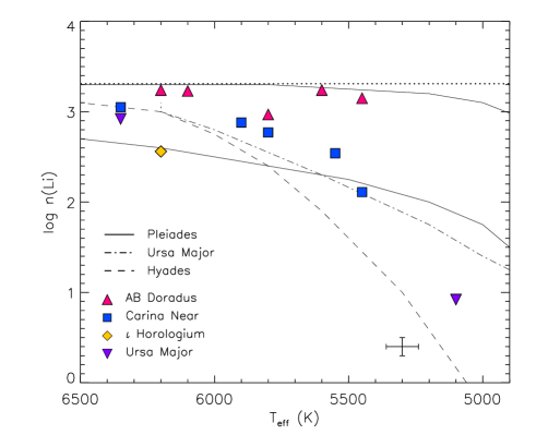
Figure 1: Lithium abundance versus effective temperature for all our sample. Typical errors in $T_{\rm eff}$ and $\log n{\rm(Li)}$ are over-plotted on the bottom-right corner of the panel. The dotted line at $\log n{\rm(Li)}=3.31$ marks the meteoritic abundance of lithium. The two solid lines represent the lower and upper limits for the Pleiades stars, while dash-dotted and dashed lines indicate the upper limits for the UMa and Hyades groups, respectively, as adopted by Zickgraf et al. (2005; see also references therein).

4.2 Abundances of iron-peak, $\alpha$-, and other elements

4.2.1 Fe

In Fig. 2 we show the iron abundance ([Fe/H]) as a function of $T_{\rm eff}$ for the three associations and for $\iota$ Hor. Since we obtain similar Fe i and Fe ii abundances for the whole sample (see Table 4 and top-left panel in Fig. 2), henceforth we will consider [Fe i/H] as iron abundance.

For the AB Dor group we derive an average iron abundance of [Fe/H]=$0.10\pm 0.03$ dex, which is well in agreement with the value of [Fe/H]=$0.04\pm 0.05$ dex reported by Viana Almeida et al. (2009). In particular, for the two stars in common with us, the differences between our values and theirs are: $\Delta T_{\rm eff}=$69 K, $\Delta\log g=$0.07 dex, $\Delta\xi=$0.27 km s^-1, $\Delta$[Fe/H]=0.06 dex (TYC 9493-838-1) and $\Delta T_{\rm eff}=$50 K, $\Delta\log g=$0.10 dex, $\Delta\xi=$0.18 km s^-1, $\Delta$[Fe/H]=$-0.02$ dex (HIP 114530). The (small) differences are within the uncertainties and they can be attributed to the different line lists and $\sigma$-clipping criteria used. In addition, the mean iron abundance we find for AB Dor (e.g., [Fe/H]=$0.10\pm 0.03$) is slightly larger than that of the Pleiades ([Fe/H]=$0.04\pm 0.03$; An et al. 2007, and references therein). However, considering possible systematic differences between abundance analysis performed in different way, this does not role out the direct link between AB Dor and Pleiades discussed by Ortega et al. (2007).

The Carina Near group shows a mean iron abundance of [Fe/H]=$0.08\pm 0.06$ dex. For the two stars in common with Desidera et al. (2006b), we find similar values both in stellar parameters and in [Fe/H].

For the UMa members, we obtain a mean iron abundance of [Fe/H]=$0.03\pm 0.02$ dex, which is close to recent results obtained through similar spectroscopic methods (see, e.g., the recent findings by Paulson & Yelda 2006). Despite the low statistics, we can cautiously highlight the small abundance scatter of the UMa group, as also claimed in a recent work (Ammler-von Eiff & Guenther 2009). We find that the (solar) iron abundance of the UMa group is very close to that of the Pleiades ([Fe/H]=$0.04\pm 0.03$; An et al. 2007, and references therein). In particular, the UMa stars in our sample were recently analysed by Paulson & Yelda (2006) and Ramírez et al. (2007) through spectroscopic methods similar to ours, and all results agree within the errors.

The planet-host star $\iota$ Hor shows [Fe/H]=$0.16\pm 0.09$ dex. The case of this star will be discussed in Section 5.3.

4.2.2 Mg, Si, Ca, and Ti

The $\alpha$-elements, such as magnesium, silicon, calcium, and titanium, are primarily produced in the aftermath of explosions of type II supernovae, with a small contribution from type Ia SNe (Woosly & Weaver 1995).

The abundances of $\alpha$-elements are listed in Table 4 and plotted in Fig. 2. The figure shows that there is no star-to-star variation for the different elements, which show solar [X/Fe] values, with the only possible exception of Ti ii, for which slight NLTE effects may be present (see D’Orazi & Randich 2009, Biazzo et al. 2011a, b, for thorough discussions on this issue). Therefore, we consider as titanium abundance the one obtained from Ti i.

The average silicon abundance we find for AB Dor is in good agreement with the results of Viana Almeida et al. (2009), who derived mean [Si/Fe]$=-0.07\pm 0.05$ dex. In particular, for the two stars in common, the mean difference is only $0.02\pm 0.04$ dex.

In $\iota$ Hor, the abundance ratios of $\alpha$-elements with respect to iron are in their solar proportions, as also found by Paulson et al. (2003) for Hyades F–K dwarfs.

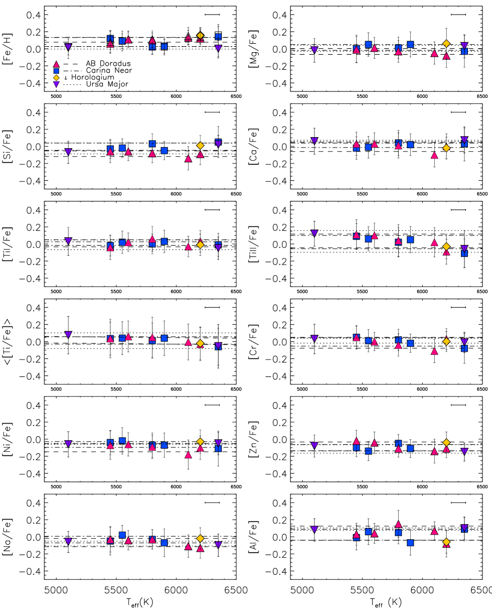
Figure 2: [Fe/H] and [X/Fe] versus $T_{\rm eff}$. In the [Fe/H] plot, filled and empty symbols refer to Fe i and Fe ii abundances, respectively. The meaning of the symbols is explained in the top-left panel. Different lines refer to regions of $\pm 1\sigma$ around the average, as indicated in the top-left panel. The horizontal error bar drawn in all plots represents the typical uncertainty in $T_{\rm eff}$.

4.2.3 Cr and Ni

Iron-peak elements are synthesised by SNIa explosions. In particular, Cr varies tighly in lockstep with iron at all [Fe/H], while Ni seems to show an upturn at [Fe/H]$>0$ (Bensby et al. 2003).

We measured the abundances of Cr and Ni as iron-peak elements; their values are plotted in Fig. 2 as a function of $T_{\rm eff}$. Also in this case, all [X/Fe] values are consistent with the solar abundances, with very small scatter (Table 4).

The average nickel abundance we derive for the AB Dor group is in good agreement with the results by Viana Almeida et al. (2009), i.e. $<$[Ni/Fe]$>=-0.06\pm 0.10$ dex. In particular, for the two stars in common with us, the mean difference is only $-0.01\pm 0.06$ dex.

4.2.4 Zn

Zinc is a volatile element which appears to behave similarly to the $\alpha$-elements.

The [Zn/Fe] ratio is slightly lower than the solar value for all associations, while for $\iota$ Hor we find solar abundance, in agreement with Paulson et al. (2003) for Hyades F–K dwarfs.

4.2.5 Na and Al

Sodium and aluminium are thought to be produced in SNe II and SNe Ib/c (Nomoto et al. 1984) as a consequence of Ne and Mg burnings in massive stars through NeNa and MgAl chains.

We plot the abundances of Na and Al relative to Fe versus $T_{\rm eff}$ in Fig. 2. The abundance ratios of Na and Al of the studied sample with respect to Fe are in their solar proportions (similar result was found by Paulson et al. 2003 for the sodium abundance of Hyades dwarfs).

5 Discussion

5.1 Elemental abundances of young associations in the Galactic disc

Each component of the Milky Way (bulge, halo, thin/thick disc) presents a characteristic elemental abundance pattern, whose differences reflect a variety of star formation histories. In our case, the small elemental abundance dispersion of the three associations studied here agrees with other recent investigations conducted both in star-forming regions (e.g., Santos et al. 2008; Biazzo et al. 2011a) and in nearby young associations (e.g., Viana Almeida et al. 2009; Ammler-von Eiff & Guenther 2009). When compared with local field stars of the thin Galactic disc (Soubiran & Girard 2005), AB Doradus, Carina Near, and Ursa Major show a similar abundance pattern. This suggests that the gas from which they formed did not undergo a peculiar enrichment, confirming the findings by Biazzo et al. (2011b; see their Fig. 10). This suggests that these nearby associations are representative of the current abundance (in all elements analysed here) of the Galactic thin disc in the solar neighbourhood.

5.2 Are nearby young associations good candidates to search for exo-planets?

The results of abundance analysis of young stars show that none of the young associations or moving groups with available metallicity determination is extremely metal-rich (see, e.g., Santos et al. 2008; Viana Almeida et al. 2009; Biazzo et al. 2011a, b; D’Orazi et al. 2011; and this work). Members of nearby young moving groups are the best targets for planet searches using direct imaging techniques. Surveys focusing on these targets were performed in the past years (e.g., Kasper et al. 2007; Chauvin et al. 2010) and next generation direct imaging instruments, like SPHERE and GPI, will also intensively observe these stars. However, it is emerging that the metallicity distribution of nearby young stars studied in direct imaging surveys is different from that of samples of radial velocity survey (e.g., Fischer & Valenti 2005). Such metallicity distribution is characterised by a significantly lower dispersion and a slightly lower mean metallicity. As suggested by Livio & Pringler (2003), metallicity may play an impotant role in the migration history of planets. Thus, the lack of nearby, young super-metal-rich stars complicates the comparison of the results of planet searches around these stars with those from radial velocity surveys. First of all, because the low metallicity dispersion of young stars makes it challenging to investigate any trend in the frequency of giant planets at wide separations with metallicity. Second, because the statistical interpretation of the results of direct imaging surveys is often done by comparing the observed frequencies or upper limits with extrapolations of the results of radial velocity surveys.

The slightly sub-solar metallicity of nearby young associations cannot be explained in terms of radial Galactocentric migration, as they are younger than $\sim 600$ Myr. In the scenario devised by Haywood (2009), giant planet formation could be favored at Galactocentric radii where the density of the molecular hydrogen, the primary constituent of planets, is higher (in particular, at the position of the molecular ring). In this case, one might expect a paucity of giant planets around young stars as compared to older stars, originating closer to the Galactic centre.

5.3 The case of $\iota$ Hor: a metal-rich planet-host star in the Hyades stream

For this target, we derive $T_{\rm eff}$=6200 K, $\log g=$4.5, [Fe i/H]=0.16$\pm$0.09 dex, [Fe ii/H]=0.15$\pm$0.09 dex, and [X/H](=[X/Fe]+[Fe/H]) higher than the Sun (see Table 4). Our values of astrophysical parameters and elemental abundances are in very good agreement with the recent literature values listed in Table 5, with the only exception of Bond et al. (2006)’s results, who found lower [Fe/H]. This agreement confirms that this star is more metal-rich than the Sun at the $\sim 2\sigma$ level. Although this is still marginally consistent with what is expected from statistical fluctuations, some discussion of this object would be merited.

As we mentioned in the Introduction, $\iota$ Hor is a young planet-host star most probably formed within the primordial Hyades star cluster and then evaporated towards the present position. Its iron abundance is very close to the value of the Hyades cluster (i.e. 0.13$\pm$0.05; Paulson et al. 2003), but also its [X/Fe] are in agreement with the mean cluster values (i.e. $<$[Na/Fe]$>$=0.01$\pm$0.09, $<$[Mg/Fe]$>$=$-$0.06$\pm$0.04, $<$[Si/Fe]$>$=0.05$\pm$0.05, $<$[Ca/Fe]$>$=0.07$\pm$0.07, $<$[Ti/Fe]$>$=0.03$\pm$0.05, $<$[Zn/Fe]$>$=$-$0.06$\pm$0.06; Paulson et al. 2003). This supports the idea that the origin of the over-metallicity and over-abundance in all other elements (i.e. [X/H]) is primordial, and not due to planet accretion, i.e. $\iota$ Hor seems to be formed together with the other Hyades stars, at the same time and in the same primordial cloud. This will have important implications both for theories of star/exoplanet formation and for cluster formation and evolution (Vauclair et al. 2008).

6 Conclusions

In this paper, we presented abundance measurements of iron-peak elements, $\alpha$-elements, and other odd-Z and even-Z elements in three young nearby associations (AB Doradus, Carina Near, and Ursa Major) and in the giant-planet host $\iota$ Horologii. To this aim, we used FEROS high-resolution spectra. Our main results can be summarised as follows:

1. Lithium abundance of all stars is consistent with their age.

2. The three associations AB Doradus, Carina Near, and Ursa Major have mean iron abundances of [Fe/H]=$0.10\pm 0.03$, $0.08\pm 0.05$, and $0.01\pm 0.01$, respectively (where the error is the standard deviation on the average). These associations are characterised by small scatter in all elemental abundances.

3. The distribution of elemental abundances of the three associations is consistent with the thin disc population of the Galaxy.

4. For $\iota$ Horologii, we find [Fe/H]=$0.16\pm 0.09$ confirming its metal-richness.

5. None of the members of the three nearby associations considered here is found to be super metal-rich (i.e. with highly super-solar metallicity). This confirms the general property of young nearby stars, i.e. that their metallicity differs from that of old, field, solar-type stars, which represent so far the most extensively planet-surveyed sample by radial velocity studies. This fact will have necessarily to be taken into account for a proper interpretation of the results of direct-imaging planet searches, whose primary targets will be young nearby stars.

Table 4: Astrophysical parameters and elemental abundances derived from our analysis.

Star

$\tiny{T_{\rm eff}}$

$\tiny{\log g}$

$\tiny{\xi}$

[Fe i/H]

[Fe ii/H]

[Na/Fe]

[Mg/Fe]

[Al/Fe]

[Si/Fe]

[Ca/Fe]

[Ti i/Fe]

[Tiii/Fe]

$<$[Ti/Fe]$>$∗

[Cr/Fe]

[Ni/Fe]

[Zn/Fe]

$EW_{\rm Li}$

$\log n{\rm(Li)}$

(K)

(km/s)

(dex)

(dex)

(dex)

(dex)

(dex)

(dex)

(dex)

(dex)

(dex)

(dex)

(dex)

(dex)

(dex)

(mÅ)

(dex)

AB Doradus

TYC 9493-838-1

5450

4.6

1.8

0.06$\pm$0.10(117)

0.08$\pm$0.13(10)

$-$0.03$\pm$0.15(3)

$-$0.01$\pm$0.15(2)

0.03$\pm$0.13(2)

$-$0.06$\pm$0.13(10)

0.03$\pm$0.14(11)

$-$0.04$\pm$0.14(13)

0.11$\pm$0.17(3)

0.04$\pm$0.23

0.05$\pm$0.13(11)

$-$0.07$\pm$0.17(35)

$-$0.02$\pm$0.12(1)

228

3.15

HIP 114530

5600

4.6

1.6

0.11$\pm$0.09(118)

0.11$\pm$0.10(10)

$-$0.04$\pm$0.11(3)

0.01$\pm$0.12(2)

0.03$\pm$0.12(2)

$-$0.06$\pm$0.11(12)

0.03$\pm$0.13(10)

0.02$\pm$0.11(12)

0.10$\pm$0.14(2)

0.06$\pm$0.18

0.00$\pm$0.11(10)

$-$0.06$\pm$0.14(38)

$-$0.04$\pm$0.12(1)

217

3.24

TYC 5155-1500-1

5800

4.6

1.9

0.10$\pm$0.09(108)

0.11$\pm$0.10(8)

$-$0.03$\pm$0.11(3)

$-$0.03$\pm$0.13(2)

0.15$\pm$0.16(2)

$-$0.08$\pm$0.11(10)

0.01$\pm$0.15(10)

0.06$\pm$0.14(12)

0.04$\pm$0.19(2)

0.05$\pm$0.24

$-$0.04$\pm$0.13(3)

$-$0.09$\pm$0.14(34)

$-$0.11$\pm$0.10(1)

143

2.97

HIP 82688

6100

4.6

1.9

0.13$\pm$0.09(54)

0.15$\pm$0.10(6)

$-$0.11$\pm$0.13(1)

$-$0.05$\pm$0.13(1)

0.07$\pm$0.11(2)

$-$0.14$\pm$0.14(7)

$-$0.10$\pm$0.14(9)

$-$0.03$\pm$0.12(7)

0.02$\pm$0.17(3)

0.00$\pm$0.21

$-$0.11$\pm$0.14(10)

$-$0.18$\pm$0.17(23)

$-$0.14$\pm$0.14(1)

142

3.23

TYC 5901-1109-1

6200

4.6

1.5

0.12$\pm$0.09(117)

0.14$\pm$0.08(10)

$-$0.13$\pm$0.12(3)

$-$0.08$\pm$0.14(2)

$-$0.08$\pm$0.16(2)

$-$0.09$\pm$0.12(11)

0.00$\pm$0.15(13)

0.03$\pm$0.13(11)

$-$0.09$\pm$0.15(2)

$-$0.03$\pm$0.19

0.03$\pm$0.12(11)

$-$0.10$\pm$0.14(34)

$-$0.11$\pm$0.11(1)

130

3.24

Average

0.10$\pm$0.03

0.12$\pm$0.03

$-$0.07$\pm$0.05

$-$0.03$\pm$0.03

0.04$\pm$0.08

$-$0.09$\pm$0.03

$-$0.01$\pm$0.05

$-$0.03$\pm$0.04

0.02$\pm$0.04

$-$0.01$\pm$0.06

$-$0.10$\pm$0.05

$-$0.08$\pm$0.05

Carina Near

HIP 37923

5450

4.6

1.5

0.12$\pm$0.09(113)

0.10$\pm$0.11(10)

$-$0.05$\pm$0.16(3)

0.00$\pm$0.16(2)

$-$0.01$\pm$0.14(2)

$-$0.03$\pm$0.11(10)

$-$0.02$\pm$0.13(10)

$-$0.02$\pm$0.12(12)

0.09$\pm$0.15(2)

0.04$\pm$0.19

0.05$\pm$0.14(10)

$-$0.04$\pm$0.14(37)

$-$0.10$\pm$0.11(1)

68

2.11

HIP 37918

5550

4.7

1.7

0.09$\pm$0.09(113)

0.09$\pm$0.12(10)

0.02$\pm$0.11(3)

0.05$\pm$0.14(2)

0.06$\pm$0.15(2)

$-$0.02$\pm$0.11(10)

$-$0.01$\pm$0.13(10)

0.02$\pm$0.13(12)

0.06$\pm$0.14(2)

0.04$\pm$0.19

0.01$\pm$0.13(10)

$-$0.02$\pm$0.16(37)

$-$0.14$\pm$0.11(1)

114

2.54

HIP 58241∗∗

5800

4.6

1.7

0.02$\pm$0.07(99)

0.03$\pm$0.07(11)

$-$0.03$\pm$0.11(3)

0.01$\pm$0.13(2)

0.05$\pm$0.13(2)

0.03$\pm$0.12(9)

0.04$\pm$0.15(11)

0.00$\pm$0.12(13)

0.02$\pm$0.17(2)

0.01$\pm$0.21

0.02$\pm$0.12(11)

$-$0.07$\pm$0.14(37)

$-$0.05$\pm$0.11(1)

113

2.77

HIP 58240

5900

4.6

1.6

0.03$\pm$0.09(114)

0.02$\pm$0.09(10)

$-$0.07$\pm$0.16(3)

0.05$\pm$0.15(2)

$-$0.07$\pm$0.14(2)

$-$0.05$\pm$0.11(10)

0.02$\pm$0.13(10)

0.03$\pm$0.13(13)

0.05$\pm$0.15(3)

0.04$\pm$0.20

$-$0.02$\pm$0.11(11)

$-$0.07$\pm$0.14(36)

$-$0.11$\pm$0.11(1)

114

2.88

HIP 36414

6350

4.5

2.4

0.14$\pm$0.12(55)

0.16$\pm$0.13(8)

$-$0.03$\pm$0.19(1)

0.09$\pm$0.14(1)

0.05$\pm$0.18(4)

0.03$\pm$0.20(6)

$-$0.01$\pm$0.14(2)

$-$0.11$\pm$0.17(2)

$-$0.06$\pm$0.22

$-$0.08$\pm$0.17(3)

$-$0.11$\pm$0.20(9)

84

3.05

Average

0.08$\pm$0.05

0.08$\pm$0.06

$-$0.03$\pm$0.04

0.02$\pm$0.03

0.02$\pm$0.06

0.00$\pm$0.04

0.01$\pm$0.03

$-$0.02$\pm$0.02

0.01$\pm$0.04

0.00$\pm$0.05

$-$0.06$\pm$0.03

$-$0.10$\pm$0.04

Ursa Major

HD 38392∗∗

5100

4.6

1.5

0.02$\pm$0.09(97)

0.01$\pm$0.13(8)

$-$0.06$\pm$0.12(1)

$-$0.02$\pm$0.14(1)

0.08$\pm$0.13(2)

$-$0.07$\pm$0.13(9)

0.06$\pm$0.15(7)

0.03$\pm$0.16(12)

0.12$\pm$0.15(1)

0.08$\pm$0.22

0.03$\pm$0.17(5)

$-$0.06$\pm$0.15(33)

$-$0.08$\pm$0.13(1)

10

0.92

HIP 27072∗∗

6350

4.3

1.6

0.00$\pm$0.09(75)

0.00$\pm$0.11(10)

$-$0.10$\pm$0.13(3)

0.03$\pm$0.14(1)

0.10$\pm$0.13(1)

0.02$\pm$0.11(8)

0.07$\pm$0.15(13)

$-$0.05$\pm$0.13(8)

$-$0.06$\pm$0.22(2)

$-$0.05$\pm$0.26

$-$0.01$\pm$0.12(10)

$-$0.05$\pm$0.13(30)

$-$0.15$\pm$0.11(1)

68

2.92

Average

0.01$\pm$0.01

0.01$\pm$0.01

$-$0.08$\pm$0.03

0.01$\pm$0.04

0.09$\pm$0.01

$-$0.03$\pm$0.06

0.07$\pm$0.01

$-$0.05$\pm$0.06

0.02$\pm$0.09

0.01$\pm$0.03

$-$0.05$\pm$0.01

$-$0.12$\pm$0.05

$\iota$ Horologii (Hyades stream)

HIP 12653

6200

4.5

1.5

0.16$\pm$0.09(111)

0.15$\pm$0.09(10)

$-$0.02$\pm$0.13(3)

0.06$\pm$0.18(1)

$-$0.06$\pm$0.13(2)

0.01$\pm$0.12(10)

$-$0.02$\pm$0.13(11)

$-$0.01$\pm$0.13(12)

$-$0.03$\pm$0.14(3)

$-$0.02$\pm$0.19

0.00$\pm$0.12(11)

$-$0.03$\pm$0.14(36)

$-$0.04$\pm$0.12(1)

38

2.56

^∗ Average of [Tii/Fe] and [Tiii/Fe].
^∗∗ The astrophysical parameters of these stars, also reported in D’Orazi et al. (2012), were revised. The results are slightly different but consistent within the errors.

Table 5: Astrophysical parameters and elemental abundances of $\iota$ Hor from the literature and from this work.

$\tiny{T_{\rm eff}}$	$\tiny{\log g}$	$\tiny{\xi}$	[Fe i/H]	[Fe ii/H]	[Na/H]	[Mg/H]	[Al/H]	[Si/H]	[Ca/H]	[Ti i/H]	[Tiii/H]	[Cr/H]	[Ni/H]	[Zn/H]	Reference
(K)		(km/s)	(dex)	(dex)	(dex)	(dex)	(dex)	(dex)	(dex)	(dex)	(dex)	(dex)	(dex)	(dex)
6150$\pm$70			0.14$\pm$0.10	0.12$\pm$0.08	0.13$\pm$0.04	0.15$\pm$0.06	0.13$\pm$0.09	0.17$\pm$0.09	0.23$\pm$0.14	0.14$\pm$0.15	0.14$\pm$0.18	0.16$\pm$0.13	0.12$\pm$0.11	0.05$\pm$0.18	Bensby et al. (2003)
6252$\pm$53	4.61$\pm$0.16	1.18$\pm$0.10	0.26$\pm$0.06												Santos et al. (2004)
					0.24$\pm$0.01	0.19$\pm$0.04	0.19$\pm$0.01								Beirão et al. (2005)
6150	4.37		0.14			0.148									Borkova & Marsakov (2005)
6097	4.34		0.11		0.08			0.10		0.07			0.07		Fischer & Valenti (2005)
6017$\pm$22	4.32$\pm$0.16	1.50$\pm$0.16	0.01$\pm$0.07		0.06$\pm$0.05		$-$0.17$\pm$0.05	0.09$\pm$0.07	0.07$\pm$0.13	$-$0.02$\pm$0.12	$-$0.03$\pm$0.06	0.03$\pm$0.04			Bond et al. (2006)
								0.19$\pm$0.05	0.17$\pm$0.11	0.26$\pm$0.07		0.16$\pm$0.07	0.19$\pm$0.06		Gilli et al. (2006)
			0.195$\pm$0.056		0.208$\pm$0.038	0.175$\pm$0.055	0.167$\pm$0.036	0.158$\pm$0.051	0.103$\pm$0.100	0.160$\pm$0.070			0.142$\pm$0.054		Gonzalez & Laws (2007)
6227$\pm$26	4.53$\pm$0.06	1.29$\pm$0.03	0.19$\pm$0.02												Sousa et al. (2008)
					0.15$\pm$0.04	0.14$\pm$0.08	0.11$\pm$0.02	0.17$\pm$0.03	0.19$\pm$0.03	0.20$\pm$0.04	0.16$\pm$0.02	0.19$\pm$0.02	0.18$\pm$0.03		Neves et al. (2009)
6080$\pm$80	4.40$\pm$0.06	0.15$\pm$0.07													Bruntt et al. (2010)
6200$\pm$60	4.5$\pm$0.1	1.5$\pm$0.1	0.16$\pm$0.09	0.15$\pm$0.09	0.14$\pm$0.09	0.21$\pm$0.16	0.10$\pm$0.10	0.17$\pm$0.08	0.14$\pm$0.09	0.15$\pm$0.09	0.13$\pm$0.12	0.16$\pm$0.08	0.13$\pm$0.11	0.12$\pm$0.09	This work

Appendix A Line list

Table 6: Wavelength, elements, excitation potential, and oscillator strength.

$\lambda$	Element	$\chi$	$\log gf$
(Å)		(eV)
5682.63	Na i	2.102	$-$0.700
6154.23	Na i	2.102	$-$1.610
6160.75	Na i	2.104	$-$1.310
7657.60	Mg i	5.110	$-$1.280
8310.30	Mg i	5.930	$-$1.090
6696.02	Al i	3.143	$-$1.499
6698.67	Al i	3.143	$-$1.950
5701.10	Si i	4.930	$-$2.050
5948.54	Si i	5.082	$-$1.230
6091.92	Si i	5.871	$-$1.400
6125.02	Si i	5.614	$-$1.570
6142.48	Si i	5.619	$-$1.480
6145.02	Si i	5.616	$-$1.440
6414.98	Si i	5.871	$-$1.100
6518.73	Si i	5.954	$-$1.500
6555.46	Si i	5.984	$-$1.000
7003.58	Si i	5.960	$-$0.870
7235.34	Si i	5.610	$-$1.510
7918.40	Si i	5.950	$-$0.610
7932.40	Si i	5.960	$-$0.470
5512.98	Ca i	2.933	$-$0.480
5581.97	Ca i	2.523	$-$0.671
5601.28	Ca i	2.526	$-$0.523
5867.56	Ca i	2.933	$-$1.610
6102.72	Ca i	1.879	$-$0.862
6122.22	Ca i	1.886	$-$0.386
6161.30	Ca i	2.523	$-$1.293
6166.44	Ca i	2.521	$-$1.156
6169.04	Ca i	2.523	$-$0.804
6169.56	Ca i	2.526	$-$0.527
6455.60	Ca i	2.523	$-$1.424
6499.65	Ca i	2.523	$-$0.818
7148.15	Ca i	2.710	0.137
7326.16	Ca i	2.930	$-$0.230
4805.42	Ti i	2.345	0.150
4820.41	Ti i	1.502	$-$0.441
4885.08	Ti i	1.887	0.358
4913.61	Ti i	1.873	0.160
5016.16	Ti i	0.848	$-$0.574
5219.70	Ti i	0.021	$-$2.292
5866.45	Ti i	1.067	$-$0.840
5953.16	Ti i	1.887	$-$0.329
5965.83	Ti i	1.879	$-$0.409
6258.10	Ti i	1.443	$-$0.431
6261.10	Ti i	1.430	$-$0.479
6743.13	Ti i	0.900	$-$1.630
7357.74	Ti i	1.440	$-$1.120
6491.56	Ti ii	2.061	$-$1.793
6606.95	Ti ii	2.061	$-$2.790
6680.13	Ti ii	3.095	$-$1.855
4936.34	Cr i	3.113	$-$0.340
5247.57	Cr i	0.961	$-$1.640
5296.69	Cr i	0.983	$-$1.400

Table 7: continued

$\lambda$	Element	$\chi$	$\log gf$
(Å)		(eV)
5300.74	Cr i	0.983	$-$2.120
5329.14	Cr i	2.914	$-$0.064
5348.31	Cr i	1.004	$-$1.290
6883.07	Cr i	3.440	$-$0.420
6925.28	Cr i	3.450	$-$0.200
6926.10	Cr i	3.450	$-$0.590
6979.80	Cr i	3.460	$-$0.220
7355.90	Cr i	2.890	$-$0.290
7400.19	Cr i	2.900	$-$0.110
4835.87	Fe i	4.103	$-$1.500
4875.88	Fe i	3.332	$-$2.020
4907.73	Fe i	3.430	$-$1.840
4999.11	Fe i	4.186	$-$1.740
5036.92	Fe i	3.017	$-$3.068
5044.21	Fe i	2.851	$-$2.059
5067.15	Fe i	4.220	$-$0.930
5141.74	Fe i	2.424	$-$2.190
5162.27	Fe i	4.178	0.020
5217.39	Fe i	3.211	$-$1.070
5228.38	Fe i	4.220	$-$1.290
5285.13	Fe i	4.434	$-$1.640
5293.96	Fe i	4.143	$-$1.870
5373.71	Fe i	4.473	$-$0.860
5386.33	Fe i	4.154	$-$1.770
5389.48	Fe i	4.415	$-$0.570
5397.62	Fe i	3.634	$-$2.480
5398.28	Fe i	4.445	$-$0.720
5472.71	Fe i	4.209	$-$1.495
5522.45	Fe i	4.209	$-$1.550
5539.28	Fe i	3.642	$-$2.660
5543.15	Fe i	3.695	$-$1.570
5543.94	Fe i	4.217	$-$1.140
5546.99	Fe i	4.217	$-$1.910
5576.09	Fe i	3.430	$-$0.894
5584.77	Fe i	3.573	$-$2.320
5636.70	Fe i	3.640	$-$2.610
5638.26	Fe i	4.220	$-$0.870
5641.43	Fe i	4.256	$-$1.063
5662.52	Fe i	4.178	$-$0.573
5691.50	Fe i	4.301	$-$1.520
5701.55	Fe i	2.559	$-$2.216
5856.09	Fe i	4.294	$-$1.570
5859.58	Fe i	4.549	$-$0.620
5862.35	Fe i	4.549	$-$0.365
5916.25	Fe i	2.453	$-$2.994
5930.18	Fe i	4.652	$-$0.251
5934.66	Fe i	3.928	$-$1.170
5956.69	Fe i	0.859	$-$4.605
5976.78	Fe i	3.943	$-$1.290
5984.81	Fe i	4.733	$-$0.280
5987.07	Fe i	4.795	$-$0.556
6003.01	Fe i	3.881	$-$1.120
6024.06	Fe i	4.548	$-$0.052
6056.01	Fe i	4.733	$-$0.460
6078.49	Fe i	4.795	$-$0.370
6137.00	Fe i	2.198	$-$2.950
6157.73	Fe i	4.076	$-$1.260
6187.99	Fe i	3.943	$-$1.720
6200.31	Fe i	2.608	$-$2.450
6315.81	Fe i	4.076	$-$1.710
6322.69	Fe i	2.588	$-$2.446
6330.85	Fe i	4.733	$-$1.158
6336.82	Fe i	3.686	$-$0.856

Table 8: continued

$\lambda$	Element	$\chi$	$\log gf$
(Å)		(eV)
6344.15	Fe i	2.433	$-$2.923
6469.19	Fe i	4.835	$-$0.770
6495.74	Fe i	4.835	$-$0.940
6498.94	Fe i	0.958	$-$4.699
6574.23	Fe i	0.990	$-$5.023
6609.11	Fe i	2.559	$-$2.692
6627.55	Fe i	4.548	$-$1.500
6703.57	Fe i	2.758	$-$3.100
6713.75	Fe i	4.790	$-$1.410
6725.36	Fe i	4.100	$-$2.210
6726.67	Fe i	4.610	$-$1.050
6733.15	Fe i	4.640	$-$1.580
6745.97	Fe i	4.070	$-$2.710
6750.16	Fe i	2.420	$-$2.655
6753.47	Fe i	4.560	$-$2.350
6786.86	Fe i	4.190	$-$1.900
6806.86	Fe i	2.730	$-$3.140
6810.27	Fe i	4.610	$-$1.000
6820.37	Fe i	4.640	$-$1.160
6839.84	Fe i	2.560	$-$3.450
6843.66	Fe i	4.550	$-$0.860
6855.72	Fe i	4.610	$-$1.710
6857.25	Fe i	4.070	$-$2.150
6858.16	Fe i	4.610	$-$0.950
6862.50	Fe i	4.560	$-$1.430
6864.31	Fe i	4.560	$-$2.290
6880.63	Fe i	4.150	$-$2.250
6898.29	Fe i	4.220	$-$2.230
6936.50	Fe i	4.610	$-$2.230
6945.20	Fe i	2.420	$-$2.460
6951.25	Fe i	4.560	$-$1.050
6960.32	Fe i	4.590	$-$1.900
6971.94	Fe i	3.020	$-$3.340
6978.86	Fe i	2.480	$-$2.490
6988.53	Fe i	2.400	$-$3.420
7000.62	Fe i	4.140	$-$2.130
7010.35	Fe i	4.590	$-$1.860
7022.96	Fe i	4.190	$-$1.110
7024.07	Fe i	4.070	$-$1.940
7038.23	Fe i	4.220	$-$1.130
7083.40	Fe i	4.910	$-$1.260
7114.56	Fe i	2.690	$-$3.930
7142.52	Fe i	4.950	$-$0.930
7219.69	Fe i	4.070	$-$1.570
7221.21	Fe i	4.560	$-$1.220
7228.70	Fe i	2.760	$-$3.270
7284.84	Fe i	4.140	$-$1.630
7306.57	Fe i	4.180	$-$1.550
7401.69	Fe i	4.190	$-$1.600
7418.67	Fe i	4.140	$-$1.440
7421.56	Fe i	4.640	$-$1.690
7447.40	Fe i	4.950	$-$0.950
7461.53	Fe i	2.560	$-$3.450
7491.66	Fe i	4.300	$-$1.010
7498.54	Fe i	4.140	$-$2.100
7507.27	Fe i	4.410	$-$1.030
7531.15	Fe i	4.370	$-$0.640
7540.44	Fe i	2.730	$-$3.750
7547.90	Fe i	5.100	$-$1.110
7551.10	Fe i	5.080	$-$1.630
7568.91	Fe i	4.280	$-$0.900
7582.12	Fe i	4.950	$-$1.600
7583.80	Fe i	3.020	$-$1.930

Table 9: continued

$\lambda$	Element	$\chi$	$\log gf$
(Å)		(eV)
7710.36	Fe i	4.220	$-$1.112
7745.52	Fe i	5.080	$-$1.140
7751.11	Fe i	4.990	$-$0.740
7807.91	Fe i	4.990	$-$0.510
7844.55	Fe i	4.830	$-$1.670
7912.87	Fe i	0.860	$-$4.850
7955.70	Fe i	5.030	$-$1.110
7959.15	Fe i	5.030	$-$1.180
5264.81	Fe ii	3.230	$-$3.120
5325.55	Fe ii	3.221	$-$3.222
5414.07	Fe ii	3.221	$-$3.750
5425.26	Fe ii	3.199	$-$3.372
5991.38	Fe ii	3.153	$-$3.560
6084.11	Fe ii	3.199	$-$3.780
6149.26	Fe ii	3.889	$-$2.800
6247.56	Fe ii	3.892	$-$2.329
6432.68	Fe ii	2.891	$-$3.685
6456.38	Fe ii	3.903	$-$2.100
6516.08	Fe ii	2.891	$-$3.450
4806.98	Ni i	3.679	$-$0.640
4852.55	Ni i	3.542	$-$1.070
4904.41	Ni i	3.542	$-$0.170
4913.97	Ni i	3.743	$-$0.630
4946.03	Ni i	3.796	$-$1.290
5003.73	Ni i	1.676	$-$3.130
5010.93	Ni i	3.635	$-$0.870
5032.72	Ni i	3.898	$-$1.270
5082.34	Ni i	3.658	$-$0.630
5155.13	Ni i	3.898	$-$0.650
5435.86	Ni i	1.986	$-$2.590
5462.49	Ni i	3.847	$-$0.930
5589.36	Ni i	3.898	$-$1.140
5593.73	Ni i	3.898	$-$0.840
5625.31	Ni i	4.089	$-$0.700
5682.20	Ni i	4.105	$-$0.499
6111.07	Ni i	4.088	$-$0.830
6175.36	Ni i	4.089	$-$0.559
6186.71	Ni i	4.105	$-$0.960
6191.17	Ni i	1.676	$-$2.353
6223.98	Ni i	4.105	$-$0.970
6378.25	Ni i	4.154	$-$0.830
6586.31	Ni i	1.951	$-$2.810
6767.78	Ni i	1.830	$-$2.060
6772.32	Ni i	3.660	$-$0.960
6842.04	Ni i	3.660	$-$1.440
7001.55	Ni i	1.930	$-$3.650
7030.02	Ni i	3.540	$-$1.700
7110.91	Ni i	1.930	$-$2.910
7381.94	Ni i	5.360	$-$0.050
7422.29	Ni i	3.630	$-$0.140
7525.12	Ni i	3.630	$-$0.670
7555.61	Ni i	3.850	$-$0.046
7574.05	Ni i	3.830	$-$0.610
7715.58	Ni i	3.700	$-$0.980
7727.62	Ni i	3.680	$-$0.300
7797.59	Ni i	3.300	$-$0.820
7826.76	Ni i	3.700	$-$1.870
4810.53	Zn i	4.078	$-$0.170

References

- Ammler-von Eiff & Guenther (2009) Ammler-von Eiff M., Guenther E. W., 2009, A&A, 508, 677
- An et al. (2007) An D., Terndrup D. M., Pinsonneault M. H., et al., 2007, ApJ, 655, 233
- Anderson et al. (2012) Anderson E., Francis Ch., 2012, AstL, 38, 331
- Asplund et al. (2009) Asplund M., Grevesse N., Sauval A. J., Scott P., 2009, ARA&A, 481, 522
- Barklem & O’Mara (1997) Barklem P. S., O’Mara B. J., 1997, MNRAS, 290, 102
- Beirão et al. (2005) Beirão P., Santos N. C., Israelian G., Mayor M., 2005, A&A, 438, 251
- Bensby et al. (2003) Bensby T., Feltzing S., Lundström I., 2003, A&A, 410, 527
- Biazzo et al. (2011a) Biazzo K., Randich S., Palla F., 2011a, A&A, 525, 35
- Biazzo et al. (2011b) Biazzo K., Randich S., Palla F., Briceño C., 2011b, A&A, 530, 19
- Bond et al. (2006) Bond J. C., Tinney C. G., Butler R. P., et al., 2006, MNRAS, 370, 163
- Borkova & Marsakov (2005) Borkova T. V., Marsakov V. A., 2005, ARep, 49, 405
- Bruntt et al. (2010) Bruntt H., Bedding T. R., Quirion P.-O., et al., 2010, MNRAS, 405, 1907
- Chauvin et al. (2010) Chauvin G., Lagrange A.-M., Bonavita M., et al., 2010, A&A, 509, 52
- Clementini et al. (2000) Clementini G., Di Tomaso S., Di Fabrizio L., et al. 2000, AJ, 120, 2054
- Cox (2000) Cox A. N., 2000, Allen’s Astrophysical Quantities, 4th edn. (New York: AIP Press and Springer-Verlag)
- D’Orazi & Randich (2009) D’Orazi V., Randich S., 2009, A&A, 501, 553
- D’Orazi et al. (2009) D’Orazi V., Randich S., Flaccomio E., et al., 2009, A&A, 501, 973
- D’Orazi et al. (2011) D’Orazi V., Biazzo K., Randich S., 2011, A&A, 526, 103
- D’Orazi et al. (2012) D’Orazi V., Biazzo K., Desidera S., Covino E., 2012, MNRAS, 423, 2789
- Desidera et al. (2006a) Desidera S., Gratton R. G., Lucatello S., et al., 2006a, A&A, 454, 553
- Desidera et al. (2006b) Desidera S., Gratton R. G., Lucatello S., Claudi R. U., 2006b, A&A, 454, 581
- Ercolano & Clarke (2010) Ercolano B., Clarke J., 2010, MNRAS, 402, 2735
- Fischer & Valenti (2005) Fischer D. A., Valenti J. 2005, ApJ, 622, 1102
- Gilli et al. (2006) Gilli G., Israelian G., Ecuvillon A., et al., 2006, 449, 723
- Gonzalez & Laws (2007) González G., Laws C., 2007, MNRAS, 378, 1141
- Gray & Corbally (2002) Gray R. O., Corbally C. J., 2002, AJ, 124, 989
- Grevesse et al. (1996) Grevesse N., Noels A., Sauval A. J.: 1996, in Cosmic Abundances, ASP Conf. Series, Vol. 99, 117
- Guillout et al. (2009) Guillout P., Klutsch A., Frasca A., et al., 2009, A&A, 504, 829
- James et al. (2006) James D. J., Melo C., Santos N. C., Bouvier J., 2006, A&A, 446, 971
- Johnson et al. (2010) Johnson J. A., Aller K. M., Howard A. W., Crepp J. R., 2010, PASP, 122, 905
- Haywood (2009) Haywood M., 2009, ApJ, 698, 1
- Kasper et al. (2007) Kasper M., Apai D., Janson M., Brandner W., 2007, A&A, 472, 321
- Kaufer et al. (1999) Kaufer A., Stahl O., Tubbesing S., et al., 1999, The Messenger, 95, 8
- Kenyon & Hartmann (1995) Kenyon S. J., Hartmann L., 1995, ApJS, 101, 117
- Kürster et al. (2000) Kürster M., Endl M., Els S., et al., 2000, A&A, 353, 33
- Kurucz (1993) Kurucz R. L.: 1993, in ATLAS9 Stellar Atmosphere Programs and 2 km s-1 grid (Kurucz CD-ROM No. 13)
- van Leeuwen (2007) van Leeuwen F., 2007, A&A, 474, 653
- Liu et al. (2012) Liu F., Chen Y. Q., Zhao G., et al., 2012, MNRAS, 422, 2969
- Livio & Pringler (2003) Livio M., Pringle J. E., 2003, MNRAS, 346, 42
- Luhman et al. (2005) Luhman K. L., Stauffer J. R., Mamajek E. E., 2005, ApJ, 628, 69
- Messina et al. (2010) Messina S., Desidera S., Turatto M., et al., 2010, A&A, 520, 15
- Montes et al. (2001) Montes D., López-Santiago J., Fernández-Figueroa M. J., Gálvez M. C., 2001, A&A, 379, 976
- Mordasini et al. (2012) Mordasini C., Alibert Y., Benz W., et al., 2012, A&A, in press
- Mouillet et al. (2010) Mouillet D., Beuzit J. L., Desidera S., et al.: 2010, in The Spirit of Lyot 2010: Direct Detection of Exoplanets and Circumstellar disks, University of Paris Diderot (France), ed. A. Boccaletti.
- Neves et al. (2009) Neves V., Santos N. C., Sousa S. G., et al., 2009, A&A, 497, 563
- Nomoto et al. (1984) Nomoto K., Thielemann F. K., Yokoi K., 1984, ApJ, 286, 644
- Ortega et al. (2007) Ortega V. G., Jilinski E., de La Reza R., Bazzanella B., 2007, MNRAS, 377, 441
- Padgett (1996) Padget D. L., 1996, ApJ, 471, 847
- Pasquini et al. (2007) Pasquini L., Bonifacio P., Randich S., et al., 2007, A&A, 464, 601
- Paulson & Yelda (2006) Paulson D. B., Yelda S., 2006, PASP, 118, 706
- Paulson et al. (2003) Paulson D. B., Sneden C., Cochran W. D., 2006, ApJ, 125, 3185
- Ramírez et al. (2007) Ramírez I., Allende Prieto C., Lambert D. L., 2007, A&A, 465, 271
- Randich et al. (2006) Randich, S., Sestito, P., Primas, F., et al., 2006, A&A, 450, 557
- Sadakane (2006) Sadakane K., 2006, PASJ, 58, 1023
- Santos et al. (2004) Santos N. C., Israelian G., Mayor M., 2004, A&A, 415, 1153
- Santos et al. (2008) Santos N. C., Melo C., James D. J., et al., 2008, A&A, 480, 889
- Santos et al. (2012) Santos N. C., Lovis C., Melendez J., et al., 2012, A&A, 538, 151
- Schlieder et al. (2012) Schlieder J. E., Lèpine S., Simon M., 2012, AJ, 143, 80
- Sneden (1973) Sneden C., 1973, ApJ, 184, 839
- da Silva et al. (2009) da Silva L., Torres C. A. O., de La Reza R., et al., 2009, A&A, 508, 833
- Soderblom et al. (1993) Soderblom D. R., Jones B. F., Balachandran S., et al., 1993, AJ, 106, 1059
- Soubiran & Girard (2005) Soubiran C., Girard P., 2005, A&A, 438, 139
- Sousa et al. (2007) Sousa S. G., Santos N. C., Israelian G., et al., 2007, A&A, 469, 783
- Sousa et al. (2008) Sousa S. G., Santos N. C., Mayor M., et al., 2008, A&A, 487, 373
- Sousa et al. (2011) Sousa S. G., Santos N. C., Israelian G., et al., 2011, A&A, 526, 99
- Steenbock & Holweger (1981) Steenbock W., Holweger H., 1981, A&A, 99, 192
- Tokovinin (2011) Tokovinin A. 2011, AJ, 141, 52
- Torres et al. (2003) Torres C. A. O., Quast G. R., de La Reza R., et al., 2003, in Galactic Star Formation Across the Stellar Mass Spectrum, ASP Conf. Series, Vol. 287, 439
- Torres et al. (2006) Torres C. A. O., Quast G. R., Da Silva L., et al., 2006, A&A, 460, 695
- Torres et al. (2008) Torres C. A. O., Quast G. R., Melo C. H. F., Sterzik M. F., 2008, in Handbook of Star Forming Regions, Vol. II, 757
- Unsöld (1955) Unsöld A.: 1955, in Physik der Sternatmosphären, Springer-Verlag, Berlin
- Vauclair et al. (2008) Vauclair S., Laymand M., Bouchy F., et al., 2008, A&A, 482, 5
- Viana Almeida et al. (2009) Viana Almeida P., Santos N. C., Melo C., et al., 2009, A&A, 501, 965
- White et al. (2007) White R. J., Gabor J. M., Hillenbrand L. A., 2007, AJ, 133, 2524
- Woosly & Weaver (1995) Woosley S. E., Weaver T. A., 1995, ApJS, 101, 181
- Yasui et al. (2010) Yasui C., Kobayashi N., Tokunaga A. T., 2010, ApJ, 723, 113
- Zickgraf et al. (2005) Zickgraf F.-J., Krautter J., Reffert S., et al., 2005, A&A, 433, 151
- Zuckerman et al. (2004) Zuckerman B., Song I., Bessell M. S., 2004, ApJ, 613, 65
- Zuckerman et al. (2006) Zuckerman B., Bessell M. S., Song I., Kim S., 2006, ApJ, 649, 115
- Zuckerman et al. (2011) Zuckerman B., Rhee J. H, Song I., Bessell M. S., 2011, ApJ, 732, 61