Ultraviolet Completions of Axigluon Models and Their Phenomenological Consequences

Abstract

The CDF and D0 collaborations have observed a forward-backward asymmetry in $t\bar{t}$ production at large invariant mass in excess of the standard model prediction. One explanation involves a heavy color octet particle with axial vector couplings to quarks (an axigluon). We describe and contrast various aspects of axigluons obtained from the breaking of a chiral $SU(3)_{L}\times SU(3)_{R}$ gauge theory both from the standpoint of a string-inspired field theory and from a quiver analysis of a local type IIa intersecting brane construction. Special attention is paid to the additional constraints and issues that arise from these classes of top-down constructions compared with the more common effective field theory approach. These include the implications of a perturbative connection to a large scale; Yukawa couplings, which must be generated from higher-dimensional operators in many constructions; anomaly cancellation, in particular the implications of the required exotics for the axigluon width, perturbativity, and the signatures from exotic decays; the possibility of family nonuniversality via mirror representations, mixing with exotics, or additional $SU(3)$ factors; the additional constraints from anomalous $U(1)$ factors in the string constructions; tadpole cancellation, which implies new uncolored matter; the prevention of string-scale masses for vector pairs; and various phenomenological issues involving FCNC, CKM constraints, and the axigluon coupling strength. It is concluded that the construction of viable axigluon models from type IIa or similar constructions is problematic and would require considerable fine tuning, but is not entirely excluded. These considerations illustrate the importance of top-down constraints on possible TeV-scale physics, independent of the ultimate explanation of the $t\bar{t}$ asymmetry.

UPR-1244-T
NSF-KITP-12-171

1 Introduction

The CDF Aaltonen:2011kc and D0 Abazov:2011rq collaborations at the Fermilab Tevatron have reported large forward-backward asymmetries in $t\bar{t}$ production. For example, CDF reports an asymmetry $A_{FB}^{t\bar{t}}=0.296\pm 0.067$ for invariant mass $M_{t\bar{t}}>450$ GeV, with an integrated luminosity of 8.7 fb^-1. This is somewhat lower than the previous value ($0.475\pm 0.114$ for 5.3 fb^-1), but is still large compared to the standard model (SM) expectation: most recent calculations, which include next-to-leading order QCD as well as electroweak corrections, are in the range $0.12-0.14$ Almeida:2008ug ; Ahrens:2011uf ; Hollik:2011ps ; Kuhn:2011ri ; Manohar:2012rs ; Bernreuther:2012sx ; Skands:2012mm ; Pagani:2012kj .

A number of possible new physics explanations have been proposed to account for the asymmetry, including the $s$-channel exchange of a heavy colored particle Ferrario:2008wm ; Martynov:2009en ; Ferrario:2009bz ; Frampton:2009rk ; Cao:2010zb ; Chivukula:2010fk ; Bai:2011ed ; Zerwekh:2011wf ; Gresham:2011pa ; Djouadi:2011aj ; Haisch:2011up ; Tavares:2011zg ; AguilarSaavedra:2011ci ; Krnjaic:2011ub ; Wang:2011hc , or the $t$ or $u$-channel exchange of a $W^{\prime}$, $Z^{\prime}$, Higgs, colored, or other particle Jung:2009jz ; Cheung:2009ch ; Shu:2009xf ; Cao:2010zb ; Cao:2011ew ; Shelton:2011hq ; Berger:2011ua ; Barger:2011ih ; Bhattacherjee:2011nr ; Grinstein:2011yv ; Grinstein:2011dz ; Patel:2011eh ; Craig:2011an ; Ligeti:2011vt ; Gresham:2011pa ; Jung:2011zv ; AguilarSaavedra:2011zy ; Fox:2011qd ; Cui:2011xy ; Duraisamy:2011pt ; Blum:2011fa ; Jung:2011id ; Ng:2011jv ; Kosnik:2011jr ; Stone:2011dn ; delaPuente:2011iu ; Wang:2011mra ; Larios:2011aa ; Hochberg:2011ru ; Ko:2012gj ; Grinstein:2012pn ; Wang:2012zv ; Duffty:2012zz ; Ayazi:2012bb ; Hagiwara:2012gy ; Allanach:2012tc ; Dupuis:2012is ; Ko:2012he with flavor changing couplings. There are stringent experimental constraints on all of these models, especially from the $t\bar{t}$ total cross section and from the LHC $t\bar{t}$ charge asymmetry $A_{C}$ (between events with the $t$ rapidity larger or smaller than that of the $\bar{t}$) Chatrchyan:2011hk ; ATLAS:2012an , both of which are consistent with the SM. Other constraints include flavor changing neutral currents (FCNC), electroweak precision tests (EWPT), dijet shapes and cross sections, and $b\bar{b}$ Bai:2011ed ; Delaunay:2012kf and lepton asymmetries Bernreuther:2012sx ; Berger:2011pu ; Berger:2012nw ; abazovD0 . The $s$-channel models are also constrained by the nonobservation of peaks in the dijet and $t\bar{t}$ cross sections Chatrchyan:2011ns ; Aad:2011fq ; Harris:2011bh ; Aad:2012wm , while the $t$ or $u$ channel models typically lead to observable effects in atomic parity violation Gresham:2012wc , associated productions such as $dG\rightarrow tW^{\prime}\rightarrow t\bar{t}d$ Chatrchyan:2012su , and $tt$ production for the (Hermitian) $Z^{\prime}$ models Cao:2011ew ; Berger:2011ua ; Aad:2012bb .

In particular, axigluon models Ferrario:2008wm ; Ferrario:2009bz ; Frampton:2009rk ; Martynov:2009en ; Chivukula:2010fk ; Cao:2010zb ; Bai:2011ed ; Tavares:2011zg ; Krnjaic:2011ub ; AguilarSaavedra:2011ci ; Wang:2011hc ; Zerwekh:2011wf ; Haisch:2011up ; Djouadi:2011aj ; Gresham:2011pa , which involve an octet of heavy colored vector bosons with axial (and possibly vector) couplings, are reasonably successful in describing the Tevatron results, though they are strongly constrained by other observations. The phenomenological aspects of such models have been extensively discussed, so here we only repeat the most essential features. The forward-backward asymmetry is mainly due to interference between the $s$-channel gluon and axigluon exchanges in $q\bar{q}\rightarrow t\bar{t}$, which is proportional to

$$A_{FB}^{t\bar{t}}(\hat{s})\propto(\hat{s}-M^{2})g_{A}^{q}g_{A}^{t},$$ (1)

where $\hat{s}$ is the CM energy-squared of the $q\bar{q}$ system, $M$ is the axigluon mass, $g_{A}^{q}$ is the axial vector coupling of the axigluon to light ($u$, $d$, $c$, $s$) quarks, and $g_{A}^{t}$ is the axial coupling to the top. Most studies have assumed a relatively heavy ($M\gtrsim(1-2)$ TeV) axigluon, so that $\hat{s}-M^{2}<0$ for the relevant kinematic region. Since $A_{FB}^{t\bar{t}}>0$ this implies opposite signs for $g_{A}^{q}$ and $g_{A}^{t}$, with relatively large magnitudes favored, e.g., $|g_{A}^{q}g_{A}^{t}|\sim(1-4)g_{s}^{2}$, where $g_{s}$ is the QCD coupling. On the other hand, the nonobservation of resonant bumps in dijet production by ATLAS Aad:2012wm and CMS Chatrchyan:2011ns suggests (e.g., Bai:2011ed ; Barcelo:2011vk ; Choudhury:2011cg ; Barcelo:2011wu ) that the axigluon should be broad, e.g., $\Gamma/M\gtrsim 20$%). This is to be compared to $\Gamma/M\sim 8-10$% expected for decays into the ordinary quarks for axial couplings $|g_{A}^{q,t,b}|=g_{s}$, vector couplings $|g_{V}^{q,t,b}|=0$, and $M\leq 2$ TeV, with the exact value depending on $M$ and $\alpha_{s}(M)$, and suggests the need for larger couplings and/or additional colored decay channels. Another possibility for enhancing the asymmetry compared to the dijet constraints is to allow family nonuniversal magnitudes, e.g., $|g_{A}^{q}|\ll|g_{A}^{t}|$ Delaunay:2011gv ; Barcelo:2011vk ; Delaunay:2012kf . Models predicting a large $A_{FB}^{t\bar{t}}$ also tend to produce a charge asymmetry $A_{C}$ larger than observed at the LHC AguilarSaavedra:2011hz ; Chatrchyan:2011hk ; ATLAS:2012an . The tension is currently less severe for the axigluons than for the $t$-channel models, but nevertheless, the correlation between $A_{FB}^{t\bar{t}}$ and $A_{C}$ could be reduced for unequal couplings to $u$ and $d$ quarks AguilarSaavedra:2012va ; Drobnak:2012cz .

One can also consider a light axigluon (e.g., $M\sim 400-450$ GeV) Tavares:2011zg , which allows a universal coupling $g_{A}^{q}=g_{A}^{t}$. In the low $M$ case, the observed asymmetry can be obtained, and the stringent limits from the modification of the $t\bar{t}$ and dijet cross sections due to axigluon exchange satisfied, provided the coupling is relatively small, e.g., $g_{A}^{q,t}\sim g_{s}/3$, and the axigluon width is large (e.g., $\Gamma/M\sim 10-20$%). A large width and weak coupling of course requires additional colored decay channels, and it was assumed that the coupling is purely axial (to avoid interference contributions to the total cross section). Very light ($M\sim 50-90$ GeV) axigluons have also been proposed Krnjaic:2011ub .

Most of the axigluon studies have been from the viewpoint of effective field theory, i.e., allowing arbitrary axigluon couplings to quarks. However, additional constraints are encountered when one considers concrete theoretical embeddings. One possibility for obtaining an axigluon is to extend the color $SU(3)$ group to chiral $SU(3)_{L}\times SU(3)_{R}$ Pati:1975ze ; Frampton:1987dn ; Frampton:1987ut ; Bagger:1987fz ; Cuypers:1990hb , which is then broken to the diagonal (vector) subgroup by the vacuum expectation value (VEV) of a scalar field transforming as $(3,3^{\ast})$. Although such an extension of the standard model or its minimal supersymmetric version (MSSM) is straightforward, it does introduce some complications in terms of anomaly cancellation and for the required properties for the gauge couplings and widths. In the family nonuniversal case there are additional challenges from Yukawa couplings and FCNC.

Further constraints arise if one attempts to obtain a chiral color extension of the MSSM from an underlying superstring construction. One important consideration, which is shared in grand unification (GUT) theories or any theory involving a perturbative connection to a large scale, is the absence of Landau poles below that scale. This strongly restricts the possibilities for the number and type of exotic fields needed for anomaly cancellation (unless the string scale is close to the TeV scale), and also for the magnitude of the axigluon coupling. We will also assume the absence of TeV-scale higher-dimensional operators except for those generated by mixing with the exotic fields.

Other considerations derive from classes of superstring constructions. We illustrate this by exploring some of the issues that arise from embedding chiral color in a type IIa quiver Cvetic:2011iq , which incorporates the local constraints of type IIa intersecting brane models (see, e.g., Blumenhagen:2005mu ; Blumenhagen:2006ci ; Cvetic:2011vz ). Perhaps the single most important new constraint is that the field content of the low energy theory is restricted to bifundamentals, adjoints, symmetric, and antisymmetric representations of non-abelian groups. Since trifundamentals are absent, tree-level quark Yukawa couplings are often forbidden. Furthermore, such constructions involve anomalous $U(1)$ factors that act like effective global symmetries at the perturbative level. These can restrict otherwise allowed couplings, and, e.g., distinguish lepton from down-Higgs supermultiplets. There are other stringy constraints from tadpole cancellation, the existence of a massless (other than the Higgs mechanism) hypercharge gauge boson, and avoiding vector pairs of fields (which typically acquire string-scale masses). These features have phenomenological consequences. This includes the need to generate the quark Yukawa couplings from higher-dimensional operators, which is especially difficult for the $t$ quark and which leads to potential difficulties with the CKM matrix, FCNC, and dilution of the axigluon axial coupling. The exotics required by anomaly cancellation and other considerations can lead to a large axigluon width, which may be desirable, but also to new constraints from the nonobservation of their decays at the LHC.

In Section 2 we will review some of these issues involving chiral color from a field theory perspective, with the additional restriction that the couplings allow a perturbative connection to a large string, compactification, or GUT scale. We mainly consider field representations that are easily obtainable from perturbative string constructions, thus eliminating trifundamental Higgs fields. Quark Yukawa couplings must then be generated by higher-dimensional operators, suggesting large ordinary-exotic mixing in the $t$ quark sector. However, for completeness we will also discuss the results of relaxing this assumption and allowing trifundamentals. The implications for the axigluon width, effective Yukawa couplings, CKM matrix, FCNC, exotic decays, and the possibilitiy of generating nonuniversal couplings through ordinary-exotic mixing are described.

In Section 3 we will extend the discussion to include the additional tadpole and massless hypercharge constraints that are required by a locally consistent type IIa intersecting brane construction, the new colorless matter suggested by those constraints, and the effective global symmetries associated with the extra anomalous $U(1)$ factors in such theories. We briefly touch on possible deformations which could prevent string scale masses for vector pairs. Our conclusion is that the construction of viable chiral color models from type IIa or similar constructions to account for the Tevatron anomaly is problematic and would require considerable fine tuning, but is not entirely excluded.

Throughout, our concern is with the general issues of constructing an axigluon model from a consistent string construction as an illustration of the importance of top-down constraints on TeV-scale physics, independent of whether the Tevatron anomaly survives. More detailed model and experimental issues are discussed in the references.

2 Field Theory Construction

We first consider the construction of a field theory model based on the gauge group $G_{\text{LR}}\equiv SU(3)_{L}\times SU(3)_{R}\times SU(2)\times U(1)_{Y}$, where $SU(3)_{L}\times SU(3)_{R}$ represents a chiral color group that will be broken to QCD, and $SU(2)\times U(1)_{Y}$ is the conventional SM electroweak group. The subscripts on the two $SU(3)$ factors indicate that the left (right)-chiral quarks of (at least) the first two families transform under $SU(3)_{L}$ ($SU(3)_{R}$), respectively. However, mirror families, exotics needed for anomaly cancellation, etc., may have different assignments. We will label scalars and left-chiral fermion fields by $(n_{L},n_{R},n_{2})_{Y}$, where $n_{L},n_{R},n_{2}$ denote respectively the $SU(3)_{L},SU(3)_{R},$ and $SU(2)$ representations, and $Y$ is the weak hypercharge. The $SU(3)_{L}\times SU(3)_{R}$ gauge interactions of quarks are

$$-\mathcal{L}=g_{L}\vec{A}^{\mu}_{L}\cdot\vec{J}_{L\mu}+g_{R}\vec{A}^{\mu}_{R}\cdot\vec{J}_{R\mu},$$ (2)

where $g_{L,R}$ are the gauge couplings, $A^{i}_{L,R}$, $i=1\cdots 8$, are the gauge bosons, and $J^{i}_{L,R}$ the currents associated with the two $SU(3)$ factors. For a single quark flavor $q$ transforming as $(3,1)+(1,3^{\ast})$ the currents are just $J^{i}_{L,R\mu}=\bar{q}L^{i}\gamma_{\mu}P_{L,R}\,q$, where $L^{i}=\lambda^{i}/2$ are the $SU(3)$ matrices and $P_{L,R}=(1\mp\gamma^{5})/2$.

The simplest assignment for a single quark family that will lead to axial vector couplings is therefore

$$Q+u^{c}+d^{c}=(3,1,2)_{1/6}+(1,3^{\ast},1)_{-2/3}+(1,3^{\ast},1)_{1/3},$$ (3)

where $Q=(u\ d)^{T}$. (We assume three canonical lepton families.) The $SU(3)_{L}\times SU(3)_{R}$ symmetry can be broken to the diagonal (vector) $SU(3)$ by introducing a Higgs field

$$\Phi=(3,3^{\ast},1)_{0},$$ (4)

which is assumed to acquire a VEV $\langle 0|\Phi|0\rangle=v_{\phi}I$, where $I$ is the $3\times 3$ identity matrix and $v_{\phi}$ can be taken real and positive. It is then straightforward to show that

$$-\mathcal{L}=g_{s}\vec{G}^{\mu}\cdot(\vec{J}_{L\mu}+\vec{J}_{R\mu})+g_{s}\vec{G}_{A}^{\mu}\cdot(\cot\delta\vec{J}_{L\mu}-\tan\delta\vec{J}_{R\mu}),$$ (5)

where $\tan\delta\equiv g_{R}/g_{L}$, $g_{s}\equiv g_{L}\sin\delta$ is the QCD coupling, $G^{i}$ are the massless QCD gluons, and $J^{i}_{L\mu}+J^{i}_{R\mu}$ is the QCD current. The $G_{A}^{i}$ are the eight axigluon fields, with mass $M_{G_{A}}\equiv M=\sqrt{g_{L}^{2}+g_{R}^{2}}\,v_{\phi}$. In general, the $G_{A}^{i}$ couple to both axial and vector currents, with the axial ($-\gamma_{\mu}\gamma^{5}$) and vector ($\gamma_{\mu}$) couplings to a $(3,1)+(1,3^{\ast})$ quark given by

$$g_{A}=\frac{1}{2}g_{s}(\cot\delta+\tan\delta)\geq g_{s}\qquad g_{V}=\frac{1}{2}g_{s}(\cot\delta-\tan\delta),$$ (6)

respectively. The special case $g_{L}=g_{R}$ yields a purely axial coupling, with $g_{A}=g_{s}$ and $M=2g_{s}v_{\phi}$.

A family universal axigluon (for the case of a light $G_{A}$) can therefore be obtained by assigning all three quark families to transform as in (3). However, we see from (6) that the required $g_{A}\sim g_{s}/3$ cannot be obtained at tree level.

A family nonuniversal axigluon model (for a heavy $G_{A}$) can be obtained by assigning the third quark family to transform as a mirror of the first two (e.g., Frampton:2009rk ),

$$t^{c}+b^{c}+Q_{3}=(3^{\ast},1,1)_{-2/3}+(3^{\ast},1,1)_{1/3}+(1,3,2)_{1/6},$$ (7)

with $Q_{3}=(t\ b)^{T}$. This leads to $g_{A}^{t}=-g_{A}^{q}$ and $g_{V}^{t}=+g_{V}^{q}$, with $g_{A}^{q}\geq g_{s}$ and $g_{V}^{q}$ given by (6).

The magnitudes of the axigluon couplings to ordinary and mirror quarks are flavor universal (e.g., $|g_{A}^{t}|=|g_{A}^{u}|=|g_{A}^{d}|$) at tree level in the two-node ($SU(3)_{L}\times SU(3)_{R}$) case. Flavor nonuniversality can be broken in extensions to $n$-node ($SU(3)^{n}$) models broken to a diagonal $SU(3)$ Chivukula:2010fk ; Zerwekh:2011wf ; Bai:2011ed or by mixing effects.

There are still serious constraints from anomalies, Yukawa couplings, exotic decays, and (for the nonuniversal case) flavor changing neutral currents (FCNC).

2.1 Anomaly Cancellation

The universal and nonuniversal versions of the model both have $SU(3)_{L}^{3}$, $SU(3)_{R}^{3}$, $SU(3)_{L}^{2}\times U(1)_{Y}$, and $SU(3)_{R}^{2}\times U(1)_{Y}$ triangle anomalies. Various massive fermion additions to cancel these anomalies have been suggested (e.g., Frampton:1987dn ) which involve additional fermions or families that are chiral under the electroweak part of the SM. One common example is to introduce a fourth family which (like the third) is a mirror of the first two with respect to $SU(3)_{L}\times SU(3)_{R}$. However, chiral exotics would have to be very heavy to have evaded direct detection, necessitating large Yukawa couplings to the Higgs and therefore Landau poles at low energy (e.g., Godbole:2009sy ). While not excluded experimentally, such Landau poles would be inconsistent with our assumption of a perturbative extension of the MSSM up to a large string scale. Chiral exotics also lead generically to unacceptably large corrections to EWPT unless delicate cancellations are present (e.g., Erler:2010sk ; Eberhardt:2012sb ).

We therefore restrict ourselves to cancelling the anomalies using quasichiral exotic fermions. These are defined as fermions that are vector under the SM gauge group, though they may be chiral under additional symmetries such as $SU(3)_{L}\times SU(3)_{R}$. Such quasichiral fermions do not require large Yukawa couplings and do not contribute at one loop to EWPT. They will typically acquire masses near the chiral (in this case $SU(3)_{L}\times SU(3)_{R}$) breaking scale. For simplicity (and to allow generation of exotic masses within our assumptions) we will only consider quasichiral exotics that are fundamental or antifundamental under the $SU(3)_{L,R}$ factors (as well as the bifundamental Higgs fields $\Phi$ and $\overline{\Phi}\equiv(3^{\ast},3,1)_{0}$). There are two very simple possibilities, which as far as we are aware have not been discussed in the literature: the anomalies for an ordinary family can be cancelled by adding a pair of exotic $SU(2)$ doublets $Q^{c}\,{}^{\prime}=(d^{c}\,{}^{\prime}\ -u^{c}\,{}^{\prime})^{T}$ and $Q^{\prime}=(u^{\prime}\ d^{\prime})^{T}$ transforming as

$$Q^{c}\,{}^{\prime}+Q^{\prime}=(3^{\ast},1,2)_{-1/6}+(1,3,2)_{1/6},$$ (8)

or by adding two pairs of $SU(2)$ singlets

$$u^{c}\,{}^{\prime}+d^{c}\,{}^{\prime}+u^{\prime}+d^{\prime}=(3^{\ast},1,1)_{-2/3}+(3^{\ast},1,1)_{1/3}+(1,3,1)_{2/3}+(1,3,1)_{-1/3}.$$ (9)

The anomalies for a mirror family could be cancelled by

$$Q_{3}^{\prime}+Q_{3}^{c}\,{}^{\prime}=(3,1,2)_{1/6}+(1,3^{\ast},2)_{-1/6}$$ (10)

or

$$t^{\prime}+b^{\prime}+t^{c}\,{}^{\prime}+b^{c}\,{}^{\prime}=(3,1,1)_{2/3}+(3,1,1)_{-1/3}+(1,3^{\ast},1)_{-2/3}+(1,3^{\ast},1)_{1/3}.$$ (11)

Of course, one can also have hybrid situations, involving some singlet and some doublet pairs. In the nonuniversal case, the anomalies of the third family cancel those of one of the light families, so it would suffice to only add one family of exotics, either (8) or (9).

There are some advantages to assuming quasichiral exotics for each family, i.e., they may allow a larger axigluon width (if the exotics are sufficiently light), and they also facilitate the generation of effective Yukawa couplings in the present framework. However, they are problematic for our assumption of perturbativity of the gauge couplings $g_{L}=g_{s}/\sin\delta$ and $g_{R}=g_{s}/\cos\delta$. Assuming three families of exotics, as well as $\Phi$ and $\overline{\Phi}$, the supersymmetric $\beta$ functions for $SU(3)_{L}$ and $SU(3)_{R}$ vanish at one-loop (see Appendix A). However, they are positive at two loops Jones:1981we ; Einhorn:1981sx , so that perturbativity up to the string scale $M_{S}$ requires a relatively low string scale and small values of $g_{L,R}$ at $M$. For $\delta=\pi/4$, one requires $M_{S}\lesssim 2\times 10^{8}M$, while smaller or larger $\delta$ (useful for phenomenological reasons as described below) require a much lower string scale, as shown in Figure 1. We will mainly consider $0.2\lesssim\delta/\pi\lesssim 0.3$, so that $M_{S}/M\gtrsim 10^{4}$.

On the other hand, for a single family of exotics in the nonuniversal case, as well as $\Phi$ and $\overline{\Phi}$, the $SU(3)_{L,R}$ couplings are asymptotically free, allowing $M_{S}$ as large as the Planck scale, provided that the initial values at $M$ are not too large. The latter restriction is satisfied for $0.1\lesssim\delta/\pi\lesssim 0.4$. We will discuss both the three and one exotic family cases below.

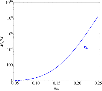
Figure 1: The maximum value of $M_{S}/M$ allowed by the assumption of perturbativity of $g_{L}$ up to the string scale $M_{S}$ as a function of $\delta=\tan^{-1}(g_{R}/g_{L})$, assuming three families of exotics plus $\Phi$ and $\overline{\Phi}$. The mixed two-loop $\beta$ function terms of $\mathcal{O}(g_{L}^{5})$ and $\mathcal{O}(g_{L}^{3}g_{R}^{2})$ are included, but the electroweak and Yukawa couplings are neglected. For $M=\mathcal{O}\,$(TeV) the maximum allowed string scale is only around $10^{11}$ GeV, and requires $\delta\sim\pi/4$ so that $g_{L}\sim g_{R}\sim\sqrt{2}g_{s}$ at $M$. The curve is symmetric around $\delta=\pi/4$, except that the roles of $g_{L}$ and $g_{R}$ are interchanged for $\delta>\pi/4$.

As will be discussed in Section 2.2, the $SU(2)$-doublet exotics are problematic for the third family, because they lead to unacceptable modifications of the CKM matrix. All of the possibilities involve some pairs that are totally vector under $G_{\text{LR}}$, such as intrafamily terms $Q+Q^{c}\,{}^{\prime}$ or $Q_{3}^{c}\,{}^{\prime}+Q_{3}$, cross family terms like $Q^{\prime}+Q_{3}^{c}\,{}^{\prime}$ or $Q_{3}^{\prime}+Q^{c}\,{}^{\prime}$, or analogous pairs involving $SU(2)$-singlet exotics. We must assume that some additional symmetries prevent such vector pairs from combining to form very heavy (e.g., string-scale) states. The role of the extra stringy conditions for these requirements will be discussed in Section 3.

2.2 Exotic Masses and Effective Yukawa Couplings

Exotic Masses

Another important complication involves the generation of masses for the ordinary and exotic quarks. Clearly, the exotic doublet pair $Q^{\prime}+Q^{c}\,{}^{\prime}$ can acquire a mass at the $SU(3)_{L}\times SU(3)_{R}\,$-breaking scale $v_{\phi}$ by a renormalizable-level Yukawa coupling $\lambda_{Q^{\prime}}\Phi\,Q^{\prime}Q^{c}\,{}^{\prime}$, while exotic singlets can acquire masses via $\lambda_{u^{\prime}}\Phi\,u^{\prime}u^{c}\,{}^{\prime}$ or $\lambda_{d^{\prime}}\Phi\,d^{\prime}d^{c}\,{}^{\prime}$. Similarly, mirror exotics can acquire masses from couplings to an additional field $\overline{\Phi}$ transforming as $(3^{\ast},3,1)_{0}$, i.e., $\lambda_{Q_{3}^{\prime}}\overline{\Phi}\,Q_{3}^{\prime}Q_{3}^{c}\,{}^{\prime}$, $\lambda_{t^{\prime}}\overline{\Phi}\,t^{\prime}t^{c}\,{}^{\prime}$, or $\lambda_{b^{\prime}}\overline{\Phi}\,b^{\prime}b^{c}\,{}^{\prime}$. In a nonsupersymmetric theory, the role of $\bar{\Phi}$ can be played by $\Phi^{\dagger}$.

Trifundamental Higgs Doublets

However, mass terms for the ordinary quarks are problematic. Renormalizable-level Yukawa couplings $H_{u}Q\,u^{c}$ or $H_{d}Q\,d^{c}$ would require Higgs doublets transforming as the trifundamental representation $(3^{\ast},3,2)_{\pm 1/2}$. As emphasized in the Introduction the trifundamental Higgs representations cannot be obtained in the types of string constructions we are considering. The assumption is generically valid in perturbative type II and type I string theory, and also in some heterotic compactifications. In F-theory it is possible to obtain trifundamental representations from three-pronged string junctions, but obtaining these representations as massless degrees of freedom is relatively difficult, since they exist at high codimension in moduli space.

However, for completeness, we briefly comment on the implications of trifundamental Higgs doublets. The main drawback is that such states would require a very complicated construction, even at the field theory level. A second set of Higgs doublets $(1,1,2)_{\pm 1/2}$ not carrying $SU(3)_{L}\times SU(3)_{R}$ charges would still be required for the Yukawa couplings of leptons, while a third set $(3,3^{\ast},2)_{\pm 1/2}$ would be required for the Yukawa couplings of a mirror generation. It would be nontrivial to arrange for all of these fields to have nonzero VEVs, though it might be possible if the different sets of doublets were connected by cubic interactions involving $\Phi$ and $\overline{\Phi}$. On the other hand, trifundamental Higgs fields would allow straightforward generation of the ordinary quark masses, with little mixing with exotic quarks required. Since such mixings tend to dilute the axial couplings, such constructions would have a better chance of describing the collider data.

$(1,1,2)_{\pm 1/2}$ Higgs Doublets

Now consider the more challenging situation in which there are no trifundamental Higgs fields. It is still possible to generate effective Yukawa interactions from higher-dimensional operators obtained by integrating out the heavy exotics (similar situations have been considered by many authors, e.g., Fox:2011qd ; Tavares:2011zg ; Shelton:2011hq ). However, there are important complications and constraints. First, it is nontrivial to obtain a large enough top quark mass. Secondly, renormalizable Yukawa interactions of $(1,1,2)_{\pm 1/2}$ Higgs doublets connecting ordinary and mirror families are allowed by the gauge symmetry. Unless they are suppressed by additional quantum numbers or other means they could lead to large CKM mixings for the third family. Finally, bare mass terms connecting normal and exotic quarks are also allowed by $G_{\text{LR}}$. Unless these are forbidden or suppressed they can lead to mixing effects that can considerably reduce the axial vector couplings of the mass-eigenstate quarks to the $G_{A}$. Large mixings of the top quark with exotics are hard to avoid within the present framework in the absence of trifundamentals, while they are model dependent for the other quarks. In addition to suppressing the axial couplings, mixing of the quark doublets $Q_{i}$ with exotic states leads to violation of CKM universality or observations, so any left-handed quark mixings must be very small. Mixing of the $Q_{i}$ with singlet exotics would also lead to off-diagonal couplings of the $Z$ and Higgs. Mixing of the antiquarks (i.e., of the right-handed quarks) with exotics is not constrained by observations of the CKM matrix, but for doublet exotics would lead to off-diagonal $Z$ and Higgs couplings and right-handed couplings of the $W$.

Three Exotic Families

We first discuss the case of three families of exotics. Consider, for example, the $u$ quark in the model with singlet exotics, as in (9). One can write renormalizable mass and mixing terms

$$-\mathcal{L}=\mathcal{M}_{s}u^{\prime}u^{c}\,{}^{\prime}+h_{s}H_{u}Qu^{c}\,{}^{\prime}+\delta_{s}u^{\prime}u^{c},$$ (12)

where $\mathcal{M}_{s}\equiv\lambda_{u^{\prime}}v_{\phi}$, $h_{s}$ is a Yukawa coupling which connects $Q$ to $u^{c}\,{}^{\prime}$, and $H_{u}$ is a Higgs doublet transforming as $(1,1,2)_{1/2}$ with VEV $v_{u}\equiv\langle H^{0}_{u}\rangle\sim 174$ GeV $\sin\beta$, where $\tan\beta\equiv v_{u}/v_{d}$. The subscripts indicate the presence of singlet exotics, and flavor indices are suppressed. The last term is an $SU(3)_{L}\times SU(3)_{R}\times SU(2)\times U(1)_{Y}$-invariant mixing. The coefficient $\delta_{s}$ could in principle be a bare mass. However, as mentioned above, it is more plausible that $\delta_{s}$ is generated by the VEV of a singlet field that breaks some additional symmetry. We will assume that $\delta_{s}$ is smaller than or of the same order as the chiral $SU(3)$ breaking. For $\mathcal{M}_{s}$ much larger than $\delta_{s}$ and $h_{s}v_{u}$ one can integrate out the exotic fields to obtain the effective Yukawa interaction $(h_{s}\delta_{s}/\mathcal{M}_{s})H_{u}Qu^{c}$, so that the $u$-quark mass is $m_{u}\sim(h_{s}\delta_{s}/\mathcal{M}_{s})v_{u}$. From the $2\times 2$ mass matrix, the left mixing $\theta_{L}$ (between $u$ and $u^{\prime}$) and right mixing $\theta_{R}$ (between $u^{c}$ and $u^{c}\,{}^{\prime}$) angles are given by

$$\theta_{L}\sim\frac{h_{s}v_{u}}{\mathcal{M}_{s}}\sim\frac{m_{u}}{\delta_{s}},\qquad\theta_{R}\sim\frac{\delta_{s}}{\mathcal{M}_{s}}.$$ (13)

In principle, $\theta_{L}$ and the analogous mixings for $d$, $s$, and $b$ lead to apparent violation of the CKM universality condition

$$|U_{ud}|^{2}+|U_{us}|^{2}+|U_{ub}|^{2}=1.$$ (14)

However, the uncertainty in the observed value $\sum_{i}|U_{ud_{i}}|^{2}=0.9999(6)$ Beringer:1900zz allows for $\theta_{L}$ as large as 0.02 (e.g., Langacker:1988ur ), with a similar limit for the $d$ quark and even weaker limits for $s$ and $b$. For $m_{u}\sim 5$ MeV this is satisfied for the very weak restriction $\delta_{s}\gtrsim 250$ MeV. The analogous constraints for the $d$, $s$ and $b$ mixing parameters are respectively 250 MeV, 1 GeV, and 5 GeV. Since $\theta_{L}$ describes mixing between a doublet and singlet it induces FCNC between the light and heavy states. However, FCNC between light states such as $u$ and $c$ is at most of second order, but can actually be negligibly small Langacker:1988ur . $\theta_{L}$ also allows for exotic decays into light quarks (Section (2.4)). $\theta_{R}$ has no effect on SM physics, but does slightly modify the axigluon couplings.

For doublet exotics, (12) is replaced by

$$-\mathcal{L}=\mathcal{M}_{d}Q^{\prime}Q^{c}\,{}^{\prime}+h_{d}H_{u}Q^{\prime}u^{c}+\delta_{d}QQ^{c}\,{}^{\prime},$$ (15)

where $\mathcal{M}_{d}=\lambda_{Q^{\prime}}v_{\phi}$ and the subscripts refer to doublet. The lightest mass eigenvalue is $m_{u}\sim h_{d}v_{u}\delta_{d}/\mathcal{M}_{d}$. This is very much like the singlet case, except that the left and right mixings are interchanged, i.e., $\theta_{L}\sim\delta_{d}/\mathcal{M}_{d}$, $\theta_{R}\sim m_{u}/\delta_{d}$, and any FCNC is in the right ($u^{c}-u^{c}\,{}^{\prime}$) sector. The CKM universality constraint on $\theta_{L}$ is satisfied for $\delta_{d}/\mathcal{M}_{d}\lesssim 0.02$ for $u$ and $d$, and $\lesssim 0.1$ for $s$.

It is therefore straightforward to generate masses for the first two quark families, as well as the $b$ quark and Cabibbo mixing, by higher-dimensional operators. The top quark, however, is more challenging. Suppose, for example, that the third family is a mirror with singlet exotics, as in (7) and (11). The relevant mass terms are

$$-\mathcal{L}=\mathcal{M}_{t}t^{\prime}t^{c}\,{}^{\prime}+h_{t}H_{u}Q_{3}t^{c}\,{}^{\prime}+\delta_{t}t^{\prime}t^{c},$$ (16)

where $\mathcal{M}_{t}=\lambda_{t^{\prime}}v_{\bar{\phi}}$. Assuming that $\mathcal{M}_{t}\gg h_{t}v_{u}$ the smaller mass eigenvalue is $m_{t}\sim h_{t}v_{u}\delta_{t}/\sqrt{\delta_{t}^{2}+\mathcal{M}_{t}^{2}}$. Unless $h_{t}v_{u}$ is quite large this requires a large value for $\delta_{t}$ and leads to significant mixing. The right-handed component of the lightest mass eigenstate is

$$t^{c}_{1}=\cos\theta_{R}t^{c}-\sin\theta_{R}t^{c}\,{}^{\prime}\sim\frac{\mathcal{M}_{t}}{\sqrt{\delta_{t}^{2}+\mathcal{M}_{t}^{2}}}t^{c}-\frac{\delta_{t}}{\sqrt{\delta_{t}^{2}+\mathcal{M}_{t}^{2}}}t^{c}\,{}^{\prime}.$$ (17)

In principle $h_{t}$ is bounded by the requirement that there are no Landau poles up to a large scale. However, as discussed in Appendix A this is difficult to quantify in this case because of the vanishing of the $\beta$ functions for $g_{L,R}$ at one loop and the rather low string scales shown in Figure 1. For the illustrative range 170 GeV $\lesssim h_{t}v_{u}\lesssim$ 450 GeV, with $m_{t}\sim 164$ GeV (the $\overline{MS}$ mass), $\cos\theta_{R}$ increases from $\sim 0.3$ to $\sim 0.9$. Note that $t_{1}^{c}$ is dominated by $t^{c}\,{}^{\prime}$ rather than $t^{c}$ for much of the range (up to $h_{t}v_{u}\sim 280$ GeV). The left-handed mixing is typically small. The axial vector coupling of the axigluon to the top quark is diluted compared to (6) by the mixing. Ignoring the left-handed mixing, the reduction factor is $\cos^{2}\theta_{R}$ (see Appendix B), reducing $A_{FB}^{t\bar{t}}$ in (1) from interference by the same amount.

We reiterate that for a mirror third family mixing terms such as $H_{u}Qt^{c},$ $H_{u}Q_{3}u^{c},$ $H_{d}Qb^{c},$ and $H_{d}Q_{3}d^{c}$ are allowed by $SU(3)_{L}\times SU(3)_{R}\times SU(2)\times U(1)_{Y}$. This is unnatural in that it is backward from observations, i.e., the CKM mixings between the third family and the first two are tiny, suggesting small mixing terms compared to the masses. Such terms would have to be strongly suppressed by new symmetries or other mechanisms such as world-sheet instanton effects to avoid large third family mixing and also the dilution of the axial axigluon couplings. Similarly, if an ordinary and mirror exotic family were both singlets or both doublets they would involve vector pairs such as $u^{\prime}+t^{c}\,{}^{\prime}$ that could acquire large masses unless they are suppressed.

One Exotic Family

Now consider the possibility of a single exotic family in the nonuniversal case. We only consider singlet exotics for the same reason as in the three family case, i.e., because doublet exotics would lead to unacceptably large left-handed top mixing. We therefore have two ordinary families $Q_{i}+u_{i}^{c}+d_{i}^{c},\,i=1,2$ of the type in (3), one mirror family $Q_{3}+u_{3}^{c}+d_{3}^{c}$, as in (7), and one exotic family $u^{c}\,{}^{\prime}+d^{c}\,{}^{\prime}+u^{\prime}+d^{\prime}$ as in (9). Note that $u_{3}^{c}$ and $u^{c}\,{}^{\prime}$ have the same quantum numbers, as do $d_{3}^{c}$ and $d^{c}\,{}^{\prime}$. We use the label $u_{3}^{c}$ rather than $t^{c}$ because the mass eigenstate antitop will actually consist mainly of $u_{2}^{c}$ and $u^{c}\,{}^{\prime}$.

The allowed mass terms in this case are

$$-\mathcal{L}=\mathcal{M}u^{\prime}u^{c}\,{}^{\prime}+h_{i}H_{u}Q_{i}u_{3}^{c}+k_{i}H_{u}Q_{i}u^{c}\,{}^{\prime}+\kappa_{i}H_{u}Q_{3}u_{i}^{c}+\delta_{i}u^{\prime}u^{c}_{i},$$ (18)

where $\mathcal{M}\equiv\lambda v_{\phi}$; the $\delta_{i}$ are bare masses or generated by singlet VEVs; and $h_{i}$, $k_{i}$, and $\kappa_{i}$, $i=1,2$, are Yukawa couplings which we assume to be perturbatively bounded. We have used the equivalence of $u_{3}^{c}$ and $u^{c}\,{}^{\prime}$ to eliminate a coupling $\mathcal{M}^{\prime}u^{\prime}u_{3}^{c}$. Consider first the limit in which $\mathcal{M},\,\delta_{2}\gg\kappa_{2}v_{u}$ and the other couplings are neglected. This is effectively the $t$-exotic system, with the lighter of the two nonzero masses $m_{t}\sim\kappa_{2}v_{u}\mathcal{M}/\sqrt{\delta_{2}^{2}+\mathcal{M}}$. The lighter eigenstate is $t_{1}\sim t\in Q_{3}$ with little left-mixing, and

$$t^{c}_{1}=\cos\theta_{R}u^{c}\,{}^{\prime}-\sin\theta_{R}\ u_{2}^{c}\sim\frac{\delta_{2}}{\sqrt{\delta_{2}^{2}+\mathcal{M}^{2}}}u^{c}\,{}^{\prime}-\frac{\mathcal{M}}{\sqrt{\delta_{2}^{2}+\mathcal{M}^{2}}}u_{2}^{c}.$$ (19)

This closely resembles (17) except that $\delta$ and $\mathcal{M}$ are interchanged. The axial coupling of the $t_{1}$ is $-g_{A}\cos^{2}\theta_{R}$. As discussed in Appendix A the absence of a Landau pole up to $M_{S}/M\sim 10^{15}$ leads to an upper bound on $\kappa_{2}v_{u}$ which increases from $\sim 170$ to $\sim 450$ GeV as $\delta/\pi$ increases from $0.1$ to $0.4$. Similar to the three exotic family case, this implies an upper bound on $\cos\theta_{R}$ which increases roughly linearly from 0.3 to 0.9 for $0.1<\delta/\pi<0.4.$

We have verified numerically that the other parameters in (18) can be adjusted to give reasonable values for the $u$ and $c$ quark masses, and that similar considerations can yield appropriate masses for the down-type quarks. The observed CKM mixing between the left-handed quarks can be reproduced (with the mixings occurring in either the up or down sector, or in a combination), with small left-mixing with $u^{\prime}$. Finally, the parameters can be chosen to maximize the axial couplings of the $u$ quark (so that its right-component is $\sim u^{c}_{1}$), while the c-quark can have nearly vector couplings (i.e., its right-component can be $\sim u^{c}_{3}$). Similar statements apply in the down sector.

2.3 Flavor Changing Neutral Currents

FCNC are a serious concern for the nonuniversal model, because any mixing between the third and light fermion families would break the GIM mechanism and generate couplings like $\bar{s}\gamma_{\mu}d$, $\bar{b}\gamma_{\mu}d$, $\bar{b}\gamma_{\mu}s$, or $\gamma_{\mu}\rightarrow\gamma_{\mu}\gamma^{5}$ to the axigluon, leading to new contributions to neutral $K$, $B_{d}$ and $B_{s}$ meson mixing. Assuming that the observed CKM mixing is mainly due to the $d,s,$ and $b$ sector, the observed $K$ and $B$ mixing eliminates most but not all of relevant the parameter space Chivukula:2010fk ; Bai:2011ed ; Haisch:2011up . This would be relaxed if the CKM mixing is dominantly due to mixing between the $u,c,$ and $t$ Bai:2011ed ; Haisch:2011up because of the weaker constraints on $D$ mixing.

Normal-exotic quark mixing can also induce FCNC between light quarks at second order, but as commented in Section 2.2 this can be negligibly small. We have not investigated FCNC mediated by the various Higgs fields in detail.

2.4 The Axigluon Width, Exotic Decays, and Universality

As mentioned in the Introduction, the various constraints from the $t\bar{t}$ and dijet cross sections are relaxed considerably if the axigluon width is large compared to the value $\Gamma/M\sim 8-10$% expected for decays into ordinary quarks only with $|g_{A}|=g_{s}$ and $g_{V}=0$. In particular, it has been emphasized that decays into an ordinary and exotic quark, $G_{A}\rightarrow qq^{c}\,{}^{\prime}+q^{c}q^{\prime}$ can increase the width if the off-diagonal couplings are sufficiently large Barcelo:2011vk ; Barcelo:2011wu . However, such couplings are proportional to mixing angles such as $\theta_{L,R}$ in (13), which we expect to be small except for the $t^{c}-t^{c}\,{}^{\prime}$ mixing. Nevertheless, a large width for decays into ordinary quarks alone can be obtained for $g_{L}\neq g_{R}$, as can be seen in Figure 2, because of the enhanced couplings in (6). Decays into exotic $q^{\prime}q^{c}\,{}^{\prime}$ pairs are not suppressed by small mixings if they are kinematically allowed, and can also significantly increase the width. E.g., $\Gamma/M\sim 15$% is obtainable for $g_{L}=g_{R}$ and a common exotic mass $m_{E}\sim M/4$ for three exotic families, and much larger widths are possible for $g_{L}\neq g_{R}$. Decays into scalar partners of the ordinary and exotic quarks, or into the states associated with $\Phi$ and $\overline{\Phi}$, could increase the width even more.

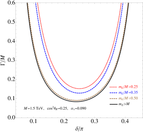
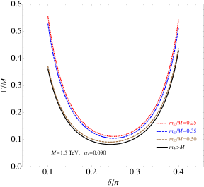
Figure 2: Left: The fractional axigluon width $\Gamma/M$ for $M=1.5$ TeV and $\alpha_{s}(M)=0.090$ as a function of $\delta=\tan^{-1}(g_{R}/g_{L})$, for decays into ordinary quarks only (solid-black line at bottom), and for decays into ordinary quarks, three families of exotic pairs, and mixing-induced $tt^{c}\,{}^{\prime}+t^{c}t^{\prime}$ pairs, which are shown for various common exotic masses $m_{E}\leq M/2$ as dotted-red, dashed-blue, and dashed-brown lines. Normal-exotic mixing is ignored except for $t^{c}-t^{c}\,{}^{\prime}$, for which we take $\cos^{2}\theta_{R}=0.25$. The $t^{c}-t^{c}\,{}^{\prime}$ mixing is most noticeable in the asymmetry between $\delta$ and $\pi/2-\delta$ for larger values of $m_{E}$. The region $0.2\lesssim\delta/\pi\lesssim 0.3$ is favored by the assumption $M_{S}/M>10^{4}$ (Figure 1). Right: $\Gamma/M$ for one family of exotic pairs. In this case, $\cos\theta_{R}$ is the largest value consistent with the absence of a Landau pole in $\kappa_{2}$ up to $M_{S}/M=10^{15}$.

A strong constraint on or possible signature of axigluon models is associated with the production and decay of the exotic quarks. These may be pair produced through ordinary QCD processes or, if they are lighter than $M/2$, through axigluon decays. They may also be produced singly in association with a light quark by axigluon decays or via a virtual $W$ or $Z$, but in these cases the rates are suppressed by (usually) small mixings. Exotic decays will often be dominated by mixing with the ordinary quarks Atre:2011ae ; Barcelo:2011wu ; Bini:2011zb , leading to $q^{\prime}\rightarrow qW$, $qZ$, or $qH$, with the $W$, $Z$, or Higgs on-shell, for which there are already significant limits Aad:2011yn ; Aad:2012en ; Aad:2012ak . In some cases there may also be cascades involving lighter exotics (especially in the doublet case) or scalar partners Kang:2007ib . These and the $\Phi$ and $\overline{\Phi}$ decays (e.g., via the couplings such as $\lambda_{u^{\prime}}u^{\prime}u^{c}\,{}^{\prime}\Phi$) have rates and characteristics strongly dependent on the various masses.

The magnitudes of the axigluon couplings are universal for ordinary or mirror quarks, i.e., for which $q_{i}$ and $q^{c}_{i}$ transform as $(3,1)+(1,3^{\ast})$ or $(3^{\ast},1)+(1,3)$: $g_{V}^{i}=g_{V}$, $g_{A}^{i}=\pm g_{A}$, where $g_{V,A}$ are given by (6). However, nonuniversal magnitudes (or off-diagonal couplings) can be induced by mixing with exotics or other quarks with different transformations, as detailed in Appendix B. Significant mixing of left-handed quarks tends to modify the CKM matrix in violation of observations, while right-handed mixings are not so constrained. We have seen that in the absence of trifundamental Higgs fields it is difficult to avoid significant top quark mixings unless Yukawas such as $h_{t}$ in (16) or $\kappa_{2}$ in (18) are quite large. We therefore restrict consideration to singlet third-family exotics so that these are in the right-handed $t^{c}-t^{c}\,{}^{\prime}$ sector. For the other quarks in the three exotic family case the mixings can be small. In particular, small $b$ quark mixing would lead to an enhanced $b\bar{b}$ asymmetry relative to $t\bar{t}$. However, it is possible to have large right-handed mixings for the lighter quarks as well, e.g., for singlet exotics if the relevant $\delta$’s in (12), (16), or their analogs for $d$, $s$, and $b$, are comparable to the $\mathcal{M}$’s. For one-exotic family some right-handed mixings must be large, but these can be restricted to the second family if desired. From (38) one sees that right-handed mixing (with $\theta_{L}$ small) has the effect of reducing the axial couplings by $\cos^{2}\theta_{R}$, while the vector couplings are increased or decreased depending on the sign of $\delta-\pi/4$. Of course, $|\cos\theta_{R}|=1$ yields a purely vector coupling $g_{s}\cot\delta\ (-g_{s}\tan\delta)$ since the left and right mass eigenstates are both associated with $SU(3)_{L}$ ($SU(3)_{R}$).

Family-nonuniversal magnitudes can also be obtained in models with one or more additional $SU(3)$ nodes (e.g., Chivukula:2010fk ; Zerwekh:2011wf ; Bai:2011ed ), which also involve additional massive colored vectors. However, additional $SU(3)$ factors would enormously complicate the constructions (and also tend to decrease the Tevatron asymmetry Chivukula:2010fk ), and will not be considered here further.

2.5 Comparison with Collider Data

Some comparison of the types of axigluon models considered here with the Tevatron and LHC data is in order. The collider and other implications of axigluon models have been extensively studied by other authors (see, e.g., Bai:2011ed ; Haisch:2011up ; Delaunay:2011gv and the other references given in the Introduction). It is not our goal to repeat those analyses. Rather, we will utilize a recent effective operator study by Delaunay et al Delaunay:2011gv of the Tevatron and LHC $t\bar{t}$ cross section and asymmetry measurements. The Tevatron data are strongly dominated by $u\bar{u}$ scattering, so the most important operators are

$$\mathcal{O}_{V}^{8}=(\bar{u}\gamma_{\mu}L^{i}u)\,(\bar{t}\gamma^{\mu}L^{i}t),\qquad\mathcal{O}_{A}^{8}=(\bar{u}\gamma_{\mu}\gamma^{5}L^{i}u)\,(\bar{t}\gamma^{\mu}\gamma^{5}L^{i}t),$$ (20)

with $\mathcal{L}=c_{V}^{8}\mathcal{O}_{V}^{8}+c_{A}^{8}\mathcal{O}_{A}^{8}$. The best fit point and allowed regions at 1 and 2$\sigma$ from the Tevatron data are reproduced in Figure 3, along with a region excluded by a recent CMS cross section measurement Chatrchyan:2012ku .

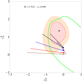
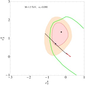
Figure 3: Left: Best fit point and allowed regions in $c_{V}^{8}$ vs. $c_{A}^{8}$ at $1\sigma$ (red) and $2\sigma$ (orange) from the Tevatron $t\bar{t}$ cross section and asymmetry measurements, and the region excluded by the CMS $t\bar{t}$ cross section (exterior of green contour), reproduced from Delaunay et al Delaunay:2011gv . The dashed contours are the predictions of the axigluon model for $M=1.5$ TeV, $\alpha_{s}(M)=0.090$, $0.1<\delta/\pi<0.4$ (with 0.4 the leftmost point on each contour), and various top mixing angles $\cos\theta_{R}$. From top to bottom, $\cos\theta_{R}=0.9$ (black), $1/\sqrt{2}$ (blue), $0.5$ (red), and $0.3$ (brown). The favored range $0.2<\delta/\pi<0.3$ are the solid parts of the contours, while $\delta/\pi=0.25$ is indicated by the filled squares. Right: Predictions of the model with one exotic family (black dashed contour) for $0.1<\delta/\pi<0.4$. For each $\delta$, $\cos\theta_{R}$ is the largest value consistent with the absence of a Landau pole in $\kappa_{2}$ up to $M_{S}/M=10^{15}$. The leftmost point is for $\delta/\pi=0.4$ and the black square corresponds to $\delta/\pi\sim 0.37$. The solid red contour also includes a $u^{c}-u^{c}_{3}$ mixing with $\cos\theta^{u}_{R}=1/\sqrt{6}$.

The coefficients $c_{V,A}^{8}$ for the heavy axigluon case correspond approximately to

$$c_{V}^{8}\sim-\frac{g_{V}^{u}\,g_{V}^{t}}{M^{2}},\qquad c_{A}^{8}\sim-\frac{g_{A}^{u}\,g_{A}^{t}}{M^{2}}$$ (21)

in our notation, where it is assumed that $\hat{s}\ll M^{2}$ and that the axigluon width can be neglected. The expected values are shown the nonuniversal case for $M=1.5$ TeV, $\alpha_{s}(M)=0.09$, $0.1<\delta/\pi<0.4$, and various fixed values for the right-handed top quark mixing $\cos\theta_{R}$ in the left-hand plot in Figure 3. It is seen that the predicted values are in good agreement for small mixings ($\cos\theta_{R}\sim 0.9$), and fall within the 2$\sigma$ contours for $\cos\theta_{R}\gtrsim 0.3$. However, the most favorable points occur for $\delta/\pi\gtrsim 0.35$ or $\lesssim 0.25$, for which either $g_{R}$ or $g_{L}$ require a rather low string scale to avoid a Landau pole for 3 exotic families (Figure 1). Restricting to the more favored range $0.2<\delta/\pi<0.3$ takes one outside of the $2\sigma$ region unless $\cos\theta_{R}$ is close to unity. The right-hand plot shows the predicted contour for the one exotic family case, assuming that the top mixing $\cos\theta_{R}$ for a given $\delta$ is the largest value consistent with $M_{S}/M=10^{15}$. Relatively large values of $\delta/\pi$ fall within the $1\sigma$ contour, both because they correspond to large $g_{R}$ and because a large $\cos\theta_{R}$ (e.g., 0.9 for $\delta/\pi\sim 0.37$) is allowed.

There are other collider constraints on axigluon models, including the $t\bar{t}$ charge asymmetry $A_{C}$, the dijet cross section, and the dijet angular distribution. These are rather model dependent, but we briefly discuss the implications of the present scenario. The current charge asymmetry measurements Chatrchyan:2011hk ; ATLAS:2012an are consistent with the standard model. These do not yet seriously constrain the axigluon model Delaunay:2011gv . However, it has been emphasized AguilarSaavedra:2012va ; Drobnak:2012cz that better agreement would be possible if one allowed unequal couplings to the $u$ and $d$ because of their different relative contributions at the Tevatron and LHC. Within the present framework $g_{A}^{d}$ could indeed be made smaller than $g_{A}^{u}$ if there were significant $d^{c}-d^{c}\,{}^{\prime}$ mixing. However, the sign could not be reversed (as favored in Drobnak:2012cz ) without invoking large left-handed mixing as well. Constraints from the dijet (or $t\bar{t}$) cross section could be reduced for a sufficiently broad axigluon (Section 2.4). However, the measured dijet angular distribution Aad:2011aj ; Chatrchyan:2012bf is a significant constraint even for a large width Haisch:2011up ; Delaunay:2011gv . One way to avoid the dijet cross section and angular distribution constraints is to assume that the axigluon couplings to the $t$ are much larger than to the $u$ Delaunay:2011gv ; Barcelo:2011vk ; Delaunay:2012kf . For example, it was argued in Delaunay:2012kf , that a ratio $g^{u}/g^{t}\sim 1/6$ would suffice, at least for axial couplings. Unfortunately, while it is straightforward to reduce $|g_{A}^{u}|$ by mixing in the present framework, there is no obvious way to significantly increase $|g_{A}^{t}|$ while keeping the gauge couplings reasonably perturbative. This is illustrated for the one exotic family case in Figure 3, where the effect of including a right-handed $u$-quark mixing $\cos\theta^{u}_{R}=1/\sqrt{6}$ (which affects both $g_{V}^{u}$ and $g_{A}^{u}$) is shown. It is seen that the effective couplings are brought close to zero, well outside the experimental region. The analogous contours in the left-hand side of Figure 3 are also brought very close to the origin, but are not shown for clarity.

2.6 Field Theory Conclusions

This Section has described some of the issues encountered in an ultraviolet-complete field theoretic description of the types of chiral $SU(3)_{L}\times SU(3)_{R}$ axigluon model that have been suggested to explain the Tevatron data. Although it is relatively easy to generate a large axigluon width, our string-inspired assumptions of no Landau poles up to a moderate or large string scale and no trifundamentals make it difficult but not impossible to generate realistic quark masses and mixings without significant reductions of the top axial coupling due to mixing. Other serious issues and constraints involve FCNC, the nonobservation of exotic decays, and the difficulty of generating family nonuniversal magnitudes of the axigluon couplings. Such constructions may still be possible, but they would require considerable tuning or extra assumptions.

In the next section we address in more detail whether such models are consistent with the stringy tadpole conditions and with the extra effective global $U(1)$ symmetries found in such constructions.

3 String Theory Construction

In Section 2 we saw that the string-motivated assumption of no trifundamental Higgs has strong implications for the structure of Yukawa couplings. In this section we consider string-motivated augmentations to the field theory constructions, which lead to additional constraints. The class of gauge theories we study are common in many regions of the string landscape, in particular weakly coupled type II orientifold compactifications. These gauge theories, often depicted by a quiver diagram, generically have (at least) three features not present in standard field theoretic constructions:

• Non-abelian unitary groups are realized as $U(N)$ rather than $SU(N)$, introducing $U(1)$’s into the theory with anomalies that are cancelled by appropriate Chern-Simons terms. One important consequence is that fields in the same representation of the non-anomalous symmetries can be quiver distinct, i.e., they can have different anomalous $U(1)$ charge, allowing one to distinguish between them and giving interesting family structure. This gives a mechanism for distinguishing between lepton and down-type Higgs doublets. Also, the anomalous $U(1)$’s impose selection rules on the superpotential which can forbid couplings in perturbation theory, though it is possible to regenerate them at suppressed scales by non-perturbative effects, such as D-instantons Blumenhagen:2006xt ; Ibanez:2006da ; Florea:2006si ; Blumenhagen:2009qh .

• The constraints on the chiral spectrum necessary for string consistency include those necessary for the absence of cubic non-abelian triangle anomalies, but also include “stringy” conditions that one would not be led to in field theory. Quivers realizing anomaly-free field theories such as the MSSM often violate these conditions. See Cvetic:2011iq for a recent discussion of these constraints and the implications for exotic matter and $Z^{\prime}$ physics.

• The string scale $M_{S}$ is the natural scale in the theory, and is typically $\mathcal{O}(M_{pl}$). Therefore, fields which form a vector pair under all symmetries of the theory typically have a very large mass and decouple from low energy physics.

We will consider the ideas of Section 2 in light of these additional ingredients and will show that they have interesting phenomenological implications.

Let us briefly describe the setup for the quivers studied in this paper. We consider four-node quivers with $U(3)_{a_{1}}\times U(3)_{a_{2}}\times U(2)_{b}\times U(1)_{c}$ gauge symmetry. Generically the (trace) $U(1)$ of $U(N)$ is anomalous, and the anomalies can be cancelled via the introduction of appropriate Chern-Simons terms. These terms appear naturally in weakly coupled type II string theory in the Wess-Zumino contribution to the D-brane effective action (the generalized Green-Schwarz mechanism). In addition, the anomalous $U(1)$ gauge bosons (and sometimes the non-anomalous ones) receive a Stuckelberg mass due to the presence of one of the Chern-Simons terms participating in anomaly cancellation. However, sometimes a non-anomalous linear combination

$$U(1)_{G}=q_{a_{1}}\,U(1)_{a_{1}}+q_{a_{2}}\,U(1)_{a_{2}}+q_{b}\,U(1)_{b}+q_{c}\,U(1)_{c}$$ (22)

remains massless. We demand that one such linear combination can be identified as weak hypercharge, so that the gauge symmetry after the Green-Schwarz mechanism lifts the anomalous $U(1)$’s is $SU(3)_{L}\times SU(3)_{R}\times SU(2)\times U(1)_{Y}$. The presence of a field $(3,3^{*},1)_{0}$ to break $SU(3)_{L}\times SU(3)_{R}$ to QCD requires $q_{a_{1}}=q_{a_{2}}$. For simplicity we study only one of the two possible hypercharge embeddings, given by $U(1)_{Y}=\frac{1}{6}U(3)_{a_{1}}+\frac{1}{6}U(3)_{a_{2}}+\frac{1}{2}U(1)_{c}$. The other is given by $U(1)_{Y}=-\frac{1}{3}U(3)_{a_{1}}-\frac{1}{3}U(3)_{a_{2}}+\frac{1}{2}U(1)_{b}$.

Two sets of constraints must be imposed. We follow the conventions of Cvetic:2011iq and refer the reader to the discussions there for more details. The first set of constraints are those necessary for tadpole cancellation, which include the cancellation of cubic non-abelian anomalies but also include some string constraints. There is a tadpole constraint for each node in the quiver, labeled by the “T-charges” $T_{a_{1}}$, $T_{a_{2}}$, $T_{b}$, and $T_{c}$. Each matter field contributes some amount to these T-charges. The tadpole conditions are that the net $T_{c}$ charge must be $0$ mod $3$ and the others must be $0$. There are also “M-charge” constraints necessary for a massless hypercharge. Matter fields contribute analogously to quantities $M_{a_{1}}$, $M_{a_{2}}$, $M_{b}$, and $M_{c}$. A massless hypercharge requires that each of the net M-charges is zero.

We take a modular approach. First we consider the possible quark and lepton/Higgs sectors for the quivers, where the former give rise to the quark sector of the MSSM upon Higgsing $SU(3)_{L}\times SU(3)_{R}$ to QCD, and the latter sector contains fields in the representations of the lepton and Higgs sector of the MSSM. Any quiver of this sort has $SU(3)_{L}^{3}$, $SU(3)_{R}^{3}$, $SU(3)_{L}^{2}\times U(1)_{Y}$ and $SU(3)_{R}^{2}\times U(1)_{Y}$ triangle anomalies. We then consider the introduction of a colored exotic sector which cancels these anomalies, as described in Section 2.1, though we rely on the presence of Chern-Simons terms to cancel the anomalies associated with the anomalous $U(1)$’s. Such a quiver is anomaly free. However, it is possible that it does not satisfy all of the conditions necessary for string consistency. We therefore add a colorless exotic sector for the purpose of satisfying these constraints and study the associated phenomenology. Such a colorless exotic sector is of course possible, though not necessary, in field theory.

We will first consider the possible standard model quark and lepton sectors, and then will introduce the possible exotic sectors which could be added for anomaly cancellation. We will then show that simple phenomenological assumptions significantly restrict the possibilities, and will study issues of effective Yukawa couplings and scales in two viable quivers. Brief comments are made on possible deformations and on matter extensions needed to satisfy the tadpole conditions.

3.1 Classification of Quiver Sectors

In this section we classify the possible standard model quark and lepton sectors, and then the possible exotic quark sectors.

3.1.1 Possible Standard Model Quark and Lepton Sectors

The possible quark and lepton sectors are independent of the choice of exotics. There are four possible realizations of an ordinary generation of quarks and four of a mirror generation, given by

label	$Q$	$u^{c}$	$d^{c}$	$T_{a_{1}}$	$T_{a_{2}}$	$T_{b}$	$T_{c}$	$M_{a_{1}}$	$M_{a_{2}}$	$M_{b}$	$M_{c}$
$G_{1}$	$(a_{1},b)$	$(\overline{a}_{2},\overline{c})$	$(\overline{a}_{2},c)$	$2$	$-2$	$3$	$0$	$0$	$0$	$-\frac{1}{2}$	$1$
$G_{2}$	$(a_{1},b)$	$(\overline{a}_{2},\overline{c})$	$\raisebox{-3.5pt}{\hbox{\rule{0.4pt}{6.5pt}\hskip-0.4pt\rule{6.5pt}{0.4pt}\hskip-6.5pt\rule[6.5pt]{6.5pt}{0.4pt}}\rule[6.5pt]{0.4pt}{0.4pt}\hskip-0.4pt\rule{0.4pt}{6.5pt}}\hskip-6.9pt\raisebox{3.0pt}{\hbox{\rule{0.4pt}{6.5pt}\hskip-0.4pt\rule{6.5pt}{0.4pt}\hskip-6.5pt\rule[6.5pt]{6.5pt}{0.4pt}}\rule[6.5pt]{0.4pt}{0.4pt}\hskip-0.4pt\rule{0.4pt}{6.5pt}}_{a_{2}}$	$2$	$-2$	$3$	$0$	$0$	$0$	$-\frac{1}{2}$	$1$
$\tilde{G}_{1}$	$(a_{1},\overline{b})$	$(\overline{a}_{2},\overline{c})$	$(\overline{a}_{2},c)$	$2$	$-2$	$-3$	$0$	$0$	$0$	$-\frac{1}{2}$	$1$
$\tilde{G}_{2}$	$(a_{1},\overline{b})$	$(\overline{a}_{2},\overline{c})$	$\raisebox{-3.5pt}{\hbox{\rule{0.4pt}{6.5pt}\hskip-0.4pt\rule{6.5pt}{0.4pt}\hskip-6.5pt\rule[6.5pt]{6.5pt}{0.4pt}}\rule[6.5pt]{0.4pt}{0.4pt}\hskip-0.4pt\rule{0.4pt}{6.5pt}}\hskip-6.9pt\raisebox{3.0pt}{\hbox{\rule{0.4pt}{6.5pt}\hskip-0.4pt\rule{6.5pt}{0.4pt}\hskip-6.5pt\rule[6.5pt]{6.5pt}{0.4pt}}\rule[6.5pt]{0.4pt}{0.4pt}\hskip-0.4pt\rule{0.4pt}{6.5pt}}_{a_{2}}$	$2$	$-2$	$-3$	$0$	$0$	$0$	$-\frac{1}{2}$	$1$

label	$Q_{3}$	$t^{c}$	$b^{c}$	$T_{a_{1}}$	$T_{a_{2}}$	$T_{b}$	$T_{c}$	$M_{a_{1}}$	$M_{a_{2}}$	$M_{b}$	$M_{c}$
$M_{1}$	$(a_{2},b)$	$(\overline{a}_{1},\overline{c})$	$(\overline{a}_{1},c)$	$-2$	$2$	$3$	$0$	$0$	$0$	$-\frac{1}{2}$	$1$
$M_{2}$	$(a_{2},b)$	$(\overline{a}_{1},\overline{c})$	$\raisebox{-3.5pt}{\hbox{\rule{0.4pt}{6.5pt}\hskip-0.4pt\rule{6.5pt}{0.4pt}\hskip-6.5pt\rule[6.5pt]{6.5pt}{0.4pt}}\rule[6.5pt]{0.4pt}{0.4pt}\hskip-0.4pt\rule{0.4pt}{6.5pt}}\hskip-6.9pt\raisebox{3.0pt}{\hbox{\rule{0.4pt}{6.5pt}\hskip-0.4pt\rule{6.5pt}{0.4pt}\hskip-6.5pt\rule[6.5pt]{6.5pt}{0.4pt}}\rule[6.5pt]{0.4pt}{0.4pt}\hskip-0.4pt\rule{0.4pt}{6.5pt}}_{a_{1}}$	$-2$	$2$	$3$	$0$	$0$	$0$	$-\frac{1}{2}$	$1$
$\tilde{M}_{1}$	$(a_{2},\overline{b})$	$(\overline{a}_{1},\overline{c})$	$(\overline{a}_{1},c)$	$-2$	$2$	$-3$	$0$	$0$	$0$	$-\frac{1}{2}$	$1$
$\tilde{M}_{2}$	$(a_{2},\overline{b})$	$(\overline{a}_{1},\overline{c})$	$\raisebox{-3.5pt}{\hbox{\rule{0.4pt}{6.5pt}\hskip-0.4pt\rule{6.5pt}{0.4pt}\hskip-6.5pt\rule[6.5pt]{6.5pt}{0.4pt}}\rule[6.5pt]{0.4pt}{0.4pt}\hskip-0.4pt\rule{0.4pt}{6.5pt}}\hskip-6.9pt\raisebox{3.0pt}{\hbox{\rule{0.4pt}{6.5pt}\hskip-0.4pt\rule{6.5pt}{0.4pt}\hskip-6.5pt\rule[6.5pt]{6.5pt}{0.4pt}}\rule[6.5pt]{0.4pt}{0.4pt}\hskip-0.4pt\rule{0.4pt}{6.5pt}}_{a_{1}}$	$-2$	$2$	$-3$	$0$	$0$	$0$	$-\frac{1}{2}$	$1$

For example, $(a_{2},b)$ is a field of representation $(1,3,2)_{Y}$ with non-zero anomalous $U(1)$ charges $Q_{a_{2}}=Q_{b}=+1$, so that (using (22)) $Y=q_{a_{2}}+q_{b}=1/6$. Of course, the 2 and $2^{\ast}$ are equivalent under $SU(2)$, so that, e.g., $(a_{2},b)$ and $(a_{2},\overline{b})$ differ only in their $Q_{b}$ charges of $+1$ or $-1$, respectively. Young tableaux are used to denote symmetric and antisymmetric representations, where the appropriate anomalous $U(1)$ charge is $\pm 2$ depending on whether or not the Young diagram has a bar.

The ordinary and mirror generations are equivalent except that $a_{1}\leftrightarrow a_{2}$. The realizations labeled with a tilde differ only by the replacement $b\rightarrow\overline{b}$. In the next section we will see that $G_{2},\tilde{G}_{2},M_{2},$ and $\tilde{M}_{2}$ introduce significant difficulties into model building, and therefore we will not consider them further.

Let us address the possible lepton/Higgs sectors. We require the presence of $L,e^{c},H_{u}$ and $H_{d}$. The differences between sectors amount to different choices for the $L$, $H_{d}$, and $H_{u}$, since $e^{c}$ can only appear as the symmetric product $\raisebox{-0.5pt}{\hbox{\rule{0.4pt}{6.5pt}\hskip-0.4pt\rule{6.5pt}{0.4pt}\hskip-6.5pt\rule[6.5pt]{6.5pt}{0.4pt}}\rule[6.5pt]{0.4pt}{0.4pt}\hskip-0.4pt\rule{0.4pt}{6.5pt}}\hskip-0.4pt\raisebox{-0.5pt}{\hbox{\rule{0.4pt}{6.5pt}\hskip-0.4pt\rule{6.5pt}{0.4pt}\hskip-6.5pt\rule[6.5pt]{6.5pt}{0.4pt}}\rule[6.5pt]{0.4pt}{0.4pt}\hskip-0.4pt\rule{0.4pt}{6.5pt}}_{c}$. The three $e^{c}$ fields together contribute $M_{c}=-4$. The up-type Higgs $(H_{u})$ representation $(1,1,2)_{\frac{1}{2}}$ can appear as $(b,c)$ or $(\overline{b},c)$, whereas the leptons $L$ and the down-type Higgs $(H_{d})$ representation $(1,1,2)_{-\frac{1}{2}}$ can appear as $(b,\overline{c})$ or $(\overline{b},\overline{c})$. We can therefore label a lepton/Higgs sector as $L_{mnop}$ where $m$, $n$, $o$, and $p$ are the number of fields transforming as $(b,c)$, $(\overline{b},c)$, $(b,\overline{c})$ and $(\overline{b},\overline{c})$, respectively. If we take $m+n=1$ and $o+p=4$, as in the MSSM, their contribution to $b$ and $c$ gives $T_{b}=m-n+o-p$, $M_{b}=\frac{3}{2}$ and $M_{c}=1$. Together with the three $e^{c}$’s, the contribution of $L_{mnop}$ is

$$T_{b}=m-n+o-p\qquad M_{b}=\frac{3}{2}\qquad M_{c}=-3.$$ (23)

It is simple to show that any given lepton/Higgs sector with the MSSM content satisfies $T_{b}^{l/H}\in\{\pm 5,\pm 3,\pm 1\}$.

There are phenomenological advantages to choosing $(m,n,o,p)=(1,0,1,3)$ or $(0,1,3,1)$, in which case, $T_{b}^{l/H}=-1$ or $+1$. These choices distinguish the three $L$ doublets from the $H_{d}$ by their $Q_{b}$ charges, at least at the perturbative level. Furthermore, $H_{u}$ and $H_{d}$ must have the same anomalous $Q_{b}$ charge to simultaneously generate the effective Yukawas described in Section 2.2 for both the charge $2/3$ and charge $-1/3$ quarks at the perturbative level (for either three or one exotic familes). Having the same $Q_{b}$ charge also prevents $H_{u}$ and $H_{d}$ from being a vector pair, thus avoiding a string-scale $\mu$ parameter. An electroweak-scale $\mu$ parameter can then be generated either by D instantons Blumenhagen:2006xt ; Ibanez:2006da or by the VEV of a standard model singlet field Cvetic:2010dz .

Upon combining any quark sector with any lepton/Higgs sector, the resulting quiver has non-zero $T_{a_{1}}$ and $T_{a_{2}}$ charge, corresponding to the presence of $SU(3)_{L,R}^{3}$ anomalies. In the subsections that follow, we will consider different colored exotic sectors that can be introduced for the purpose of anomaly cancellation.

3.1.2 Possible Exotic Quarks

The exotic quarks of Section 2 can be realized as

label	$u^{c}\,{}^{\prime}$	$d^{c}\,{}^{\prime}$	$u^{\prime}$	$d^{\prime}$	$T_{a_{1}}$	$T_{a_{2}}$	$T_{b}$	$T_{c}$	$M_{a_{1}}$	$M_{a_{2}}$	$M_{b}$	$M_{c}$
$G_{E}^{1}$	$(\overline{a}_{1},\overline{c})$	$(\overline{a}_{1},c)$	$(a_{2},c)$	$(a_{2},\overline{c})$	$-2$	$2$	$0$	$0$	$0$	$0$	$0$	$0$
$G_{E}^{2}$	$(\overline{a}_{1},\overline{c})$	$(\overline{a}_{1},c)$	$(a_{2},c)$	$\overline{\raisebox{-3.5pt}{\hbox{\rule{0.4pt}{6.5pt}\hskip-0.4pt\rule{6.5pt}{0.4pt}\hskip-6.5pt\rule[6.5pt]{6.5pt}{0.4pt}}\rule[6.5pt]{0.4pt}{0.4pt}\hskip-0.4pt\rule{0.4pt}{6.5pt}}}\hskip-6.9pt\raisebox{3.0pt}{\hbox{\rule{0.4pt}{6.5pt}\hskip-0.4pt\rule{6.5pt}{0.4pt}\hskip-6.5pt\rule[6.5pt]{6.5pt}{0.4pt}}\rule[6.5pt]{0.4pt}{0.4pt}\hskip-0.4pt\rule{0.4pt}{6.5pt}}_{a_{2}}$	$-2$	$2$	$0$	$3$	$0$	$0$	$0$	$0$
$G_{E}^{3}$	$(\overline{a}_{1},\overline{c})$	$\raisebox{-3.5pt}{\hbox{\rule{0.4pt}{6.5pt}\hskip-0.4pt\rule{6.5pt}{0.4pt}\hskip-6.5pt\rule[6.5pt]{6.5pt}{0.4pt}}\rule[6.5pt]{0.4pt}{0.4pt}\hskip-0.4pt\rule{0.4pt}{6.5pt}}\hskip-6.9pt\raisebox{3.0pt}{\hbox{\rule{0.4pt}{6.5pt}\hskip-0.4pt\rule{6.5pt}{0.4pt}\hskip-6.5pt\rule[6.5pt]{6.5pt}{0.4pt}}\rule[6.5pt]{0.4pt}{0.4pt}\hskip-0.4pt\rule{0.4pt}{6.5pt}}_{a_{1}}$	$(a_{2},c)$	$(a_{2},\overline{c})$	$-2$	$2$	$0$	$0$	$0$	$0$	$0$	$0$
$G_{E}^{4}$	$(\overline{a}_{1},\overline{c})$	$\raisebox{-3.5pt}{\hbox{\rule{0.4pt}{6.5pt}\hskip-0.4pt\rule{6.5pt}{0.4pt}\hskip-6.5pt\rule[6.5pt]{6.5pt}{0.4pt}}\rule[6.5pt]{0.4pt}{0.4pt}\hskip-0.4pt\rule{0.4pt}{6.5pt}}\hskip-6.9pt\raisebox{3.0pt}{\hbox{\rule{0.4pt}{6.5pt}\hskip-0.4pt\rule{6.5pt}{0.4pt}\hskip-6.5pt\rule[6.5pt]{6.5pt}{0.4pt}}\rule[6.5pt]{0.4pt}{0.4pt}\hskip-0.4pt\rule{0.4pt}{6.5pt}}_{a_{1}}$	$(a_{2},c)$	$\overline{\raisebox{-3.5pt}{\hbox{\rule{0.4pt}{6.5pt}\hskip-0.4pt\rule{6.5pt}{0.4pt}\hskip-6.5pt\rule[6.5pt]{6.5pt}{0.4pt}}\rule[6.5pt]{0.4pt}{0.4pt}\hskip-0.4pt\rule{0.4pt}{6.5pt}}}\hskip-6.9pt\raisebox{3.0pt}{\hbox{\rule{0.4pt}{6.5pt}\hskip-0.4pt\rule{6.5pt}{0.4pt}\hskip-6.5pt\rule[6.5pt]{6.5pt}{0.4pt}}\rule[6.5pt]{0.4pt}{0.4pt}\hskip-0.4pt\rule{0.4pt}{6.5pt}}_{a_{2}}$	$-2$	$2$	$0$	$3$	$0$	$0$	$0$	$0$

label	$t^{c}\,{}^{\prime}$	$b^{c}\,{}^{\prime}$	$t^{\prime}$	$b^{\prime}$	$T_{a_{1}}$	$T_{a_{2}}$	$T_{b}$	$T_{c}$	$M_{a_{1}}$	$M_{a_{2}}$	$M_{b}$	$M_{c}$
$M_{E}^{1}$	$(\overline{a}_{2},\overline{c})$	$(\overline{a}_{2},c)$	$(a_{1},c)$	$(a_{1},\overline{c})$	$2$	$-2$	$0$	$0$	$0$	$0$	$0$	$0$
$M_{E}^{2}$	$(\overline{a}_{2},\overline{c})$	$(\overline{a}_{2},c)$	$(a_{1},c)$	$\overline{\raisebox{-3.5pt}{\hbox{\rule{0.4pt}{6.5pt}\hskip-0.4pt\rule{6.5pt}{0.4pt}\hskip-6.5pt\rule[6.5pt]{6.5pt}{0.4pt}}\rule[6.5pt]{0.4pt}{0.4pt}\hskip-0.4pt\rule{0.4pt}{6.5pt}}}\hskip-6.9pt\raisebox{3.0pt}{\hbox{\rule{0.4pt}{6.5pt}\hskip-0.4pt\rule{6.5pt}{0.4pt}\hskip-6.5pt\rule[6.5pt]{6.5pt}{0.4pt}}\rule[6.5pt]{0.4pt}{0.4pt}\hskip-0.4pt\rule{0.4pt}{6.5pt}}_{a_{1}}$	$2$	$-2$	$0$	$3$	$0$	$0$	$0$	$0$
$M_{E}^{3}$	$(\overline{a}_{2},\overline{c})$	$\raisebox{-3.5pt}{\hbox{\rule{0.4pt}{6.5pt}\hskip-0.4pt\rule{6.5pt}{0.4pt}\hskip-6.5pt\rule[6.5pt]{6.5pt}{0.4pt}}\rule[6.5pt]{0.4pt}{0.4pt}\hskip-0.4pt\rule{0.4pt}{6.5pt}}\hskip-6.9pt\raisebox{3.0pt}{\hbox{\rule{0.4pt}{6.5pt}\hskip-0.4pt\rule{6.5pt}{0.4pt}\hskip-6.5pt\rule[6.5pt]{6.5pt}{0.4pt}}\rule[6.5pt]{0.4pt}{0.4pt}\hskip-0.4pt\rule{0.4pt}{6.5pt}}_{a_{2}}$	$(a_{1},c)$	$(a_{1},\overline{c})$	$2$	$-2$	$0$	$0$	$0$	$0$	$0$	$0$
$M_{E}^{4}$	$(\overline{a}_{2},\overline{c})$	$\raisebox{-3.5pt}{\hbox{\rule{0.4pt}{6.5pt}\hskip-0.4pt\rule{6.5pt}{0.4pt}\hskip-6.5pt\rule[6.5pt]{6.5pt}{0.4pt}}\rule[6.5pt]{0.4pt}{0.4pt}\hskip-0.4pt\rule{0.4pt}{6.5pt}}\hskip-6.9pt\raisebox{3.0pt}{\hbox{\rule{0.4pt}{6.5pt}\hskip-0.4pt\rule{6.5pt}{0.4pt}\hskip-6.5pt\rule[6.5pt]{6.5pt}{0.4pt}}\rule[6.5pt]{0.4pt}{0.4pt}\hskip-0.4pt\rule{0.4pt}{6.5pt}}_{a_{2}}$	$(a_{1},c)$	$\overline{\raisebox{-3.5pt}{\hbox{\rule{0.4pt}{6.5pt}\hskip-0.4pt\rule{6.5pt}{0.4pt}\hskip-6.5pt\rule[6.5pt]{6.5pt}{0.4pt}}\rule[6.5pt]{0.4pt}{0.4pt}\hskip-0.4pt\rule{0.4pt}{6.5pt}}}\hskip-6.9pt\raisebox{3.0pt}{\hbox{\rule{0.4pt}{6.5pt}\hskip-0.4pt\rule{6.5pt}{0.4pt}\hskip-6.5pt\rule[6.5pt]{6.5pt}{0.4pt}}\rule[6.5pt]{0.4pt}{0.4pt}\hskip-0.4pt\rule{0.4pt}{6.5pt}}_{a_{1}}$	$2$	$-2$	$0$	$3$	$0$	$0$	$0$	$0$

label	$Q^{\prime}$	$Q^{c}\,{}^{\prime}$	$T_{a_{1}}$	$T_{a_{2}}$	$T_{b}$	$T_{c}$	$M_{a_{1}}$	$M_{a_{2}}$	$M_{b}$	$M_{c}$
$G_{E}^{d}$	$(a_{2},b)$	$(\overline{a}_{1},\overline{b})$	$-2$	$2$	$0$	$0$	$0$	$0$	$0$	$0$
$\tilde{G}_{E}^{d}$	$(a_{2},\overline{b})$	$(\overline{a}_{1},b)$	$-2$	$2$	$0$	$0$	$0$	$0$	$0$	$0$
$M_{E}^{d}$	$(a_{1},b)$	$(\overline{a}_{2},\overline{b})$	$2$	$-2$	$0$	$0$	$0$	$0$	$0$	$0$
$\tilde{M}_{E}^{d}$	$(a_{1},\overline{b})$	$(\overline{a}_{2},b)$	$2$	$-2$	$0$	$0$	$0$	$0$	$0$	$0$

where $\overline{\raisebox{-3.5pt}{\hbox{\rule{0.4pt}{6.5pt}\hskip-0.4pt\rule{6.5pt}{0.4pt}\hskip-6.5pt\rule[6.5pt]{6.5pt}{0.4pt}}\rule[6.5pt]{0.4pt}{0.4pt}\hskip-0.4pt\rule{0.4pt}{6.5pt}}}\hskip-6.9pt\raisebox{3.0pt}{\hbox{\rule{0.4pt}{6.5pt}\hskip-0.4pt\rule{6.5pt}{0.4pt}\hskip-6.5pt\rule[6.5pt]{6.5pt}{0.4pt}}\rule[6.5pt]{0.4pt}{0.4pt}\hskip-0.4pt\rule{0.4pt}{6.5pt}}_{a_{2}}$ is the antisymmetric product of two $3^{\ast}$’s. The first two tables involve exotic quarks which are singlets of $SU(2)$, and the third involves $SU(2)$ doublet exotics (denoted by the superscript $d$).

3.2 Simplifying Assumptions

In this section we make a number of reasonable assumptions which significantly reduce the number of viable axigluon quivers. First consider the case of three exotic families.

1. The singlet exotic generations $G_{E}^{2,3,4}$ and $M_{E}^{2,3,4}$ contain fields which transform as antisymmetric tensors and carry charge $\pm 2$ under $U(1)_{a_{1}}$ or $U(1)_{a_{2}}$. Couplings of such exotics to $\Phi$ or $\overline{\Phi}$ are forbidden by anomalous $U(1)$’s at the perturbative level, preventing the large exotic mass terms such as $\mathcal{M}_{s}u^{\prime}u^{c}\,{}^{\prime}$ in (12). We therefore we do not consider these generations. We rename $G_{E}^{s}\equiv G_{E}^{1}$ and $M_{E}^{s}\equiv M_{E}^{1}$ for convenience, where the $s$ denotes that the exotics are singlets of $SU(2)$.

2. The generations $G_{2},\tilde{G}_{2},M_{2},\tilde{M}_{2}$ also contain $d^{c}$ or $b^{c}$ fields which transform as antisymmetric tensor representations. The anomalous $U(1)$ charge forbids perturbative couplings analogous to those in Section 2.2 for $u^{c}$ or $t^{c}$. This makes the generation of standard model quark Yukawa couplings as effective operators even more difficult, and therefore we do not consider these generations. We rename $G\equiv G_{1}$, $\tilde{G}\equiv\tilde{G}_{1}$, $M\equiv M_{1}$, and $\tilde{M}\equiv\tilde{M}_{1}$.

3. The quiver symmetries $a_{1}\leftrightarrow a_{2}$ and $b\leftrightarrow\overline{b}$ introduce redundancies when building colored sectors. For example, $GGG$ and $\tilde{G}\tilde{G}\tilde{G}$ are equivalent under $b\leftrightarrow\overline{b}$. Utilizing these symmetries, it is sufficient to consider $GGG,GG\tilde{G},GGM,G\tilde{G}M,GG\tilde{M},$ and $G\tilde{G}\tilde{M}$.

4. There are two ways to realize each of the standard model Higgs doublets: $H_{u}\sim(b,c)$, $\tilde{H}_{u}\sim(\overline{b},c)$, $H_{d}\sim(b,\overline{c})$ and $\tilde{H}_{d}\sim(\overline{b},\overline{c})$, where the tilde denotes the sign under $U(1)_{b}$. We will allow for the possibility of extensions of the MSSM spectrum involving additional Higgs pairs. However, we do not consider any models in which two distinct types of Higgs, e.g., $H_{d}$ and $\tilde{H}_{d}$, must both be present and have nonzero VEVs to generate all of the needed Yukawas. This implies that only one type of the fields needs to be present, either $H_{u,d}$ or $\tilde{H}_{u,d}$. That allows the pairs $GG_{E}^{s}$, $GG_{E}^{d}$, $\tilde{G}G_{E}^{d}$, $MM_{E}^{s}$, $MM_{E}^{d}$, and $\tilde{M}M_{E}^{d}$ if one works with $\tilde{H}_{u,d}$. Similarly, it allows $\tilde{G}G_{E}^{s}$, $G\tilde{G}_{E}^{d}$, $\tilde{G}\tilde{G}_{E}^{d}$, $\tilde{M}M_{E}^{s}$, $M\tilde{M}_{E}^{d}$, and $\tilde{M}\tilde{M}_{E}^{d}$ for $H_{u,d}$. We must consider both cases since we have already utilized the quiver symmetry $b\leftrightarrow\overline{b}$ to reduce the number of colored sectors.

5. The observed limits on the $V_{tb}$ strongly disfavor the doublet exotics $\tilde{M}_{E}^{d}$ and $M_{E}^{d}$. The only remaining generation assignments are $GG_{E}^{s}$, $GG_{E}^{d}$, $\tilde{G}G_{E}^{d}$, and $MM_{E}^{s}$ for $\tilde{H}_{u,d}$. For $H_{u,d}$ the possibilities are $\tilde{G}G_{E}^{s}$, $G\tilde{G}_{E}^{d}$, $\tilde{G}\tilde{G}_{E}^{d}$, and $\tilde{M}M_{E}^{s}$.

6. All of the remaining generations with singlet exotics, $GG_{E}^{s}$, $\tilde{G}G_{E}^{s}$, $MM_{E}^{s}$, and $\tilde{M}M_{E}^{s}$, have vector pairs such as $u^{\prime}u^{c}$ or $t^{\prime}t^{c}$. However, these could be rendered quasichiral by adding an additional $U(1)$ node, leading to $\delta_{s,t}$ terms. Similarly, the generations $GG_{E}^{d}$ and $\tilde{G}\tilde{G}_{E}^{d}$ involve vector $QQ^{c}\,{}^{\prime}$ pairs. Making these quasichiral would require an extra $U(2)$ node. That would enormously complicate the construction, so we will not consider such generations further. On the other hand, the $QQ^{c}\,{}^{\prime}$ pairs in $G\tilde{G}_{E}^{d}$ and $\tilde{G}G_{E}^{d}$ are quasichiral already, carrying a net $b$ charge or $+2$ or $-2$, respectively. They could presumably acquire mass non-perturbatively or by coupling to singlet fields $\overline{S}\equiv\overline{\raisebox{-3.5pt}{\hbox{\rule{0.4pt}{6.5pt}\hskip-0.4pt\rule{6.5pt}{0.4pt}\hskip-6.5pt\rule[6.5pt]{6.5pt}{0.4pt}}\rule[6.5pt]{0.4pt}{0.4pt}\hskip-0.4pt\rule{0.4pt}{6.5pt}}\hskip-6.9pt\raisebox{3.0pt}{\hbox{\rule{0.4pt}{6.5pt}\hskip-0.4pt\rule{6.5pt}{0.4pt}\hskip-6.5pt\rule[6.5pt]{6.5pt}{0.4pt}}\rule[6.5pt]{0.4pt}{0.4pt}\hskip-0.4pt\rule{0.4pt}{6.5pt}}}_{b}$ or $S\equiv\raisebox{-3.5pt}{\hbox{\rule{0.4pt}{6.5pt}\hskip-0.4pt\rule{6.5pt}{0.4pt}\hskip-6.5pt\rule[6.5pt]{6.5pt}{0.4pt}}\rule[6.5pt]{0.4pt}{0.4pt}\hskip-0.4pt\rule{0.4pt}{6.5pt}}\hskip-6.9pt\raisebox{3.0pt}{\hbox{\rule{0.4pt}{6.5pt}\hskip-0.4pt\rule{6.5pt}{0.4pt}\hskip-6.5pt\rule[6.5pt]{6.5pt}{0.4pt}}\rule[6.5pt]{0.4pt}{0.4pt}\hskip-0.4pt\rule{0.4pt}{6.5pt}}_{b}$, respectively, leading to the $\delta_{d}$ terms. We have not attempted to construct a potential, but it is reasonable to assume that the VEVs would be comparable to or smaller than those of $\Phi$ and $\overline{\Phi}$ (and similarly for the new VEVs in the deformed models with an extra $U(1)$ node).

7. The remaining possibilities with three exotic families are to either: (a) construct the three generations using combinations of $GG_{E}^{s}$, $\tilde{G}G_{E}^{d}$, and $MM_{E}^{s}$ with $\tilde{H}_{u,d}$; or (b) utilize the combinations of $\tilde{G}G_{E}^{s}$, $G\tilde{G}_{E}^{d}$, and $\tilde{M}M_{E}^{s}$ with $H_{u,d}$. In both cases, one is subject to the constraints in item # 3. We will focus on the cases with one mirror family, which corresponds to a heavy axigluon. The possibilities are then: (a) $(GG_{E}^{s})^{2}(MM_{E}^{s})$, $(GG_{E}^{s})(\tilde{G}G_{E}^{d})(MM_{E}^{s})$; or (b) $(G\tilde{G}_{E}^{d})^{2}(\tilde{M}M_{E}^{s})$, $(G\tilde{G}_{E}^{d})(\tilde{G}G_{E}^{s})(\tilde{M}M_{E}^{s})$. There are some phenomenological differences between the various possible combinations, especially concerning the off-diagonal quark mixing terms and possible exotic decays. However, in all of these possibilities except $(G\tilde{G}_{E}^{d})^{2}(\tilde{M}M_{E}^{s})$ the fields in $M_{E}^{s}$ and $G_{E}^{s}$ form vector pairs, and this difficulty would persist for the simplest version of the deformed model with an extra $U(1)$ node. We will therefore focus on the $(G\tilde{G}_{E}^{d})^{2}(\tilde{M}M_{E}^{s})$ example, involving two families of doublet exotics and one mirror family of singlets.

Similar simplifications apply to the model with one exotic family. The unique case involving singlet exotics and for which all of the couplings in (18) are allowed is $(GG_{E}^{s})\,GM$ with $\tilde{H}_{u,d}$. This can be viewed as the limit of the $(GG_{E}^{s})^{2}(MM_{E}^{s})$ model after integrating out the heavy vector pairs in $G_{E}^{s}M_{E}^{s}$.

3.3 Quiver with Three Families of Exotics

In this section we look in detail at the quiver with a colored and exotic sector given by $GG\tilde{M}\tilde{G}_{E}^{d}\tilde{G}_{E}^{d}M_{E}^{s}$. The Higgs sector is of the $H_{u,d}$ type. Requiring that $L$ and $H_{d}$ can be distinguished, the lepton sector is fixed up top possible extensions needed to cancel the T and M charges. The fields in the quiver transform as

Standard Model: $$2\times Q\sim(a_{1},b) 1\times Q_{3}\sim(a_{2},\overline{b})$$

$$2\times d^{c}\sim(\overline{a}_{2},c) 1\times b^{c}\sim(\overline{a}_{1},c)$$

$$2\times u^{c}\sim(\overline{a}_{2},\overline{c}) 1\times t^{c}\sim(\overline{a}_{1},\overline{c})\vspace{1cm}$$

$$H_{u}\sim(b,c) H_{d}\sim(b,\overline{c})$$

$$3\times L\sim(\overline{b},\overline{c}) 3\times e^{c}\sim\raisebox{-0.5pt}{\hbox{\rule{0.4pt}{6.5pt}\hskip-0.4pt\rule{6.5pt}{0.4pt}\hskip-6.5pt\rule[6.5pt]{6.5pt}{0.4pt}}\rule[6.5pt]{0.4pt}{0.4pt}\hskip-0.4pt\rule{0.4pt}{6.5pt}}\hskip-0.4pt\raisebox{-0.5pt}{\hbox{\rule{0.4pt}{6.5pt}\hskip-0.4pt\rule{6.5pt}{0.4pt}\hskip-6.5pt\rule[6.5pt]{6.5pt}{0.4pt}}\rule[6.5pt]{0.4pt}{0.4pt}\hskip-0.4pt\rule{0.4pt}{6.5pt}}_{c}$$

Exotics: $$2\times Q^{\prime}\sim(a_{2},\overline{b}) 2\times Q^{c}\,{}^{\prime}\sim(\overline{a}_{1},b)$$

$$1\times t^{c}\,{}^{\prime}\sim(\overline{a}_{2},\overline{c}) 1\times t^{\prime}\sim(a_{1},c)$$

$$1\times b^{c}\,{}^{\prime}\sim(\overline{a}_{2},c) 1\times b^{\prime}\sim(a_{1},\overline{c})$$

$$1\times\Phi\sim(a_{1},\overline{a}_{2}) 1\times\overline{\Phi}\sim(\overline{a}_{1},a_{2}).$$ (24)

The subscript on $Q_{3}$ denotes that it is the third generation quark doublet. We will see that the structure of anomalous $U(1)$’s affects the scales of the parameters $\mathcal{M}_{d}$, $h_{d}$, and $\delta_{d}$ appearing in (15). We will change the coupling names slightly to distinguish between up-type and down-type couplings.

The anomalous $U(1)$ symmetries and possible instanton effects can alter the Yukawa couplings. The off-diagonal standard model quark Yukawa couplings $H_{u}Qt^{c}$, $H_{d}Qb^{c}$, $H_{u}Q_{3}u^{c}$, and $H_{d}Q_{3}d^{c}$ are gauge invariant under $G_{\text{LR}}=SU(3)_{L}\times SU(3)_{R}\times SU(2)\times U(1)_{Y}$. The first two carry anomalous $U(1)_{b}$ charge and are forbidden in perturbation theory. It is possible that they are generated non-perturbatively by D-instanton effects, however, in which case they would be naturally suppressed. The latter two couplings are present in perturbation theory. Depending on moduli vacuum expectation values in a string compactification, they could become hierarchical due to worldsheet instanton effects in type IIa, for example, though they can also be $\mathcal{O}(1)$.

The standard model Yukawa couplings $H_{u}Qu^{c}$, $H_{d}Qd^{c}$, $H_{u}Q_{3}t^{c}$ and $H_{d}Q_{3}b^{c}$ are not invariant under $G_{\text{LR}}$ and must be obtained as effective operators. Following Section 2.2 and changing coupling subscripts for clarity, the first two can be obtained from the $G_{\text{LR}}$ invariant couplings

$$h_{d}\,H_{d}Q^{\prime}d^{c}\qquad h_{u}\,H_{u}Q^{\prime}u^{c}\qquad\mathcal{M}_{Q}Q^{\prime}Q^{c}\,{}^{\prime}\qquad\delta_{Q}QQ^{c}\,{}^{\prime},$$ (25)

where the first three are present in perturbation theory and the last carries anomalous $U(1)_{b}$ charge and must be generated non-perturbatively. The scale of $M_{Q}$ is set by $v_{\phi}\sim\mathcal{O}(TeV)$ and therefore these fields are present in the low energy spectrum. It is convenient that $\delta_{Q}$ is naturally suppressed, however, since otherwise it would acquire a string scale mass and decouple. The Yukawa couplings $h_{d}$ and $h_{u}$ can be $\mathcal{O}(1)$ or smaller.

The third generation standard model Yukawa couplings $H_{u}Q_{3}t^{c}$ and $H_{d}Q_{3}b^{c}$ can be obtained as effective operators from the $G_{\text{LR}}$ invariant couplings

$$h_{b}\,H_{d}Q_{3}b^{c}\,{}^{\prime}\qquad\mathcal{M}_{b}b^{\prime}b^{c}\,{}^{\prime}\qquad\delta_{b}b^{c}b^{\prime}$$

$$h_{t}\,H_{u}Q_{3}t^{c}\,{}^{\prime}\qquad\mathcal{M}_{t}t^{\prime}t^{c}\,{}^{\prime}\qquad\delta_{t}t^{c}t^{\prime}.$$ (26)

$h_{b}$ and $h_{t}$ are allowed in perturbation theory and can therefore be $\mathcal{O}(1)$. The masses $\mathcal{M}_{b}$ and $\mathcal{M}_{t}$ are set by $v_{\phi}$. However, $\delta_{b}$ and $\delta_{t}$ are present in perturbation theory (i.e., $b^{c}b^{\prime}$ and $t^{c}t^{\prime}$ are vector pairs) and therefore are generically of order the string scale, so that the associated fields decouple. This is a significant drawback, which we will attempt to remedy.

In addition, the pairs $(u^{c},t^{c}\,{}^{\prime})$, $(d^{c},b^{c}\,{}^{\prime})$, and $(Q^{\prime},Q_{3})$ have the same quantum numbers. Since the couplings $u^{c}t^{\prime}$, $d^{c}b^{\prime}$ and $Q_{3}Q^{c}\,{}^{\prime}$ are linear in the redundant fields, a field redefinition can rotate them away. This is not true of $H_{u}Q_{3}u^{c}$, $H_{d}Q_{3}d^{c}$, $H_{u}Q^{\prime}t^{c}\,{}^{\prime}$, and $H_{d}Q^{\prime}b^{c}\,{}^{\prime}$, however, and they can lead to small CKM mixing of the third family with the first two. Finally, the $\mu$-term is perturbatively forbidden and can be generated at a suppressed scale by D-instantons Blumenhagen:2006xt ; Ibanez:2006da .

The problem of the string-scale $\delta_{b,t}$ can be fixed via a simple deformation of the above quiver involving an additional $U(1)_{d}$ node with hypercharge

$$U(1)_{Y}=\frac{1}{6}U(1)_{a_{1}}+\frac{1}{6}U(1)_{a_{2}}+\frac{1}{2}U(1)_{c}+\frac{1}{2}U(1)_{d}.$$ (27)

Let the singlet quark exotics and Higgs doublets in (3.3) transform under $U(1)_{d}$ rather than $U(1)_{c}$, by replacing $c$ with $d$ and $\overline{c}$ with $\overline{d}$. The representation theory of the quiver with respect to $G_{\text{LR}}$ has not changed, but the anomalous $U(1)$ charges of the fields have changed. The couplings $h_{d}$, $h_{u}$, $\delta_{b}$, and $\delta_{t}$ are now forbidden in perturbation theory because they are protected by a symmetry, but small values such as $\delta_{t}=\mathcal{O}(v_{\phi})$ can still be generated by D-instantons. The same applies to the $G_{\text{LR}}$-invariant standard model Yukawa couplings, which now carry anomalous $U(1)$ charge. The redundancy between $Q_{3}$ and $Q^{\prime}$ is still present, but not between $u^{c}$ and $t^{c}\,{}^{\prime}$ or $d^{c}$ and $b^{c}\,{}^{\prime}$. $Q_{3}Q^{c}\,{}^{\prime}$ can still be rotated away, while $H_{u}Q^{\prime}t^{c}\,{}^{\prime}$ and $H_{d}Q^{\prime}b^{c}\,{}^{\prime}$ (and $H_{u}Q_{3}t^{c}$ or $H_{d}Q_{3}b^{c}$ if they are generated by D instantons) can still lead to small CKM mixings.

Let us discuss the field content. While this quiver is consistent as a quantum field theory (with the addition of Chern-Simons terms to cancel abelian and/or mixed anomalies) it does not satisfy the conditions necessary for tadpole cancellation. Specifically, all of the T-charge and M-charge conditions are satisfied except for $T_{b}=2$, when for consistency it must be zero. There are only two ways that matter could be added for the sake of consistency without overshooting the tadpole in the other direction. The first is to add two fields transforming as $\overline{b}$, which in this case means a quasichiral pair of fields $(\overline{b},c)$ and $(\overline{b},\overline{c})$. These additions have the quantum numbers of a pair of lepton doublets which are vector like with respect to $G_{\text{LR}}$ Cvetic:2011iq . The second possibility is to add a single field $\raisebox{-3.5pt}{\hbox{\rule{0.4pt}{6.5pt}\hskip-0.4pt\rule{6.5pt}{0.4pt}\hskip-6.5pt\rule[6.5pt]{6.5pt}{0.4pt}}\rule[6.5pt]{0.4pt}{0.4pt}\hskip-0.4pt\rule{0.4pt}{6.5pt}}\hskip-6.9pt\raisebox{3.0pt}{\hbox{\rule{0.4pt}{6.5pt}\hskip-0.4pt\rule{6.5pt}{0.4pt}\hskip-6.5pt\rule[6.5pt]{6.5pt}{0.4pt}}\rule[6.5pt]{0.4pt}{0.4pt}\hskip-0.4pt\rule{0.4pt}{6.5pt}}_{b}$. This singlet couples to $LQ_{3}d^{c}$ and $LLe_{L}^{c}$ in perturbation theory and therefore could dynamically give rise to $R$-parity violating operators.

Finally, the mass term $\Phi\overline{\Phi}$ of the axigluon Higgs fields will never become charged under an anomalous $U(1)$ symmetry, and therefore these fields naturally have a high mass. In particular, the vector pair is not lifted by the deformation we have performed, and there is no deformation which will do so while retaining the same $G_{\text{LR}}$ representations for $\Phi$ and $\overline{\Phi}$. One option would be to add additional $SU(3)$ factors to the gauge group, but this would significantly complicate the construction. The mass of $\Phi\overline{\Phi}$ is a significant drawback of these constructions.

3.4 Quiver with One Exotic Family

In this section we look in detail at the quiver with a colored and exotic sector given by $GGMG_{E}^{s}$. This quiver only has one family of exotics, as discussed in Section 2.2, and can be viewed as the limit of $(GG_{E}^{s})^{2}(MM_{E}^{s})$ after decoupling the vector pairs in $G_{E}^{s}M_{E}^{s}$. The Higgs sector is of the $\tilde{H}_{u,d}$ type, and we again require that $L$ and $H_{d}$ can be distinguished. Up to possible extensions needed to cancel the T and M charges, the fields are

Standard Model: $$2\times Q_{i}\sim(a_{1},b) 1\times Q_{3}\sim(a_{2},b)$$

$$2\times d_{i}^{c}\sim(\overline{a}_{2},c) 1\times d_{3}^{c}\sim(\overline{a}_{1},c)$$

$$2\times u_{i}^{c}\sim(\overline{a}_{2},\overline{c}) 1\times u_{3}^{c}\sim(\overline{a}_{1},\overline{c})\vspace{1cm}$$

$$H_{u}\sim(\overline{b},c) H_{d}\sim(\overline{b},\overline{c})$$

$$3\times L\sim(b,\overline{c}) 3\times e^{c}\sim\raisebox{-0.5pt}{\hbox{\rule{0.4pt}{6.5pt}\hskip-0.4pt\rule{6.5pt}{0.4pt}\hskip-6.5pt\rule[6.5pt]{6.5pt}{0.4pt}}\rule[6.5pt]{0.4pt}{0.4pt}\hskip-0.4pt\rule{0.4pt}{6.5pt}}\hskip-0.4pt\raisebox{-0.5pt}{\hbox{\rule{0.4pt}{6.5pt}\hskip-0.4pt\rule{6.5pt}{0.4pt}\hskip-6.5pt\rule[6.5pt]{6.5pt}{0.4pt}}\rule[6.5pt]{0.4pt}{0.4pt}\hskip-0.4pt\rule{0.4pt}{6.5pt}}_{c}$$

Exotics: $$1\times u^{c}\,{}^{\prime}\sim(\overline{a}_{1},\overline{c}) 1\times u^{\prime}\sim(a_{2},c)$$

$$1\times d^{c}\,{}^{\prime}\sim(\overline{a}_{1},c) 1\times d^{\prime}\sim(a_{2},\overline{c})$$

$$1\times\Phi\sim(a_{1},\overline{a}_{2}) 1\times\overline{\Phi}\sim(\overline{a}_{1},a_{2}).$$ (28)

The anomalous $U(1)$’s and possible D instantons affect the scales of the parameters $\mathcal{M}$, $h_{i}$, $k_{i}$, $\kappa_{i}$, and $\delta_{i}$ appearing in (18) and therefore the quark masses and mixing angles. From Section 2.2 the relevant mass terms are

$$\mathcal{M}_{u}u^{\prime}u^{c}\,{}^{\prime},\,\,\,\,\,h_{u_{i}}H_{u}Q_{i}u_{3}^{c},\,\,\,\,\,k_{u_{i}}H_{u}Q_{i}u^{c}\,{}^{\prime},\,\,\,\,\,\kappa_{u_{i}}H_{u}Q_{3}u_{i}^{c},\,\,\,\,\,\,\,\,\,\,\delta_{u_{i}}u^{\prime}u^{c}_{i}$$

$$\mathcal{M}_{d}d^{\prime}d^{c}\,{}^{\prime},\,\,\,\,\,h_{d_{i}}H_{d}Q_{i}d_{3}^{c},\,\,\,\,\,k_{d_{i}}H_{d}Q_{i}d^{c}\,{}^{\prime},\,\,\,\,\,\kappa_{d_{i}}H_{d}Q_{3}d_{i}^{c},\,\,\,\,\,\,\,\,\,\,\delta_{d_{i}}d^{\prime}d^{c}_{i},$$ (29)

where we have changed the subscripts slightly for clarity. All of these couplings are uncharged under the anomalous $U(1)$ and are present in perturbation theory. The couplings of $h$-type, $k$-type, and $\kappa$-type can be hierarchical due to worldsheet instanton effects in type IIa string theory, for example, though they can also be $\mathcal{O}(1)$. The scales of $\mathcal{M}_{d}$ and $\mathcal{M}_{u}$ are set by $v_{\phi}$. However, the $\delta$-type mixing terms are string scale and the associated fields can be integrated out at low energies. An analogous problem existed for some $\delta$-terms in Section 3.3. Note that the fields $u_{3}^{c}$ and $u^{c}\,{}^{\prime}$, and also $d_{3}^{c}$ and $d^{c}\,{}^{\prime}$, have identical quantum numbers. The couplings we have discussed are linear in these redundant fields, however, so it is possible define a linear combination which rotates some of the terms away. We will not discuss this in detail, since a deformation can lift the redundancy.

We can again perform a simple deformation to avoid string-scale masses by adding an additional $U(1)_{d}$ node with the hypercharge given by (27). We again choose the singlet quark exotics in (3.4) to transform under $U(1)_{d}$ rather than $U(1)_{c}$. The masses $\delta_{d_{i}}$ and $\delta_{u_{i}}$ are now forbidden in perturbation theory but can be generated by D-instantons. In this case it is phenomenologically preferable to continue to associate the Higgs doublets with $U(1)_{c}$, i.e., $H_{u}=(\overline{b},c)$, $H_{d}=(\overline{b},\overline{c})$. Then, the $\kappa_{u_{i}}$ and $\kappa_{d_{i}}$ terms are allowed perturbatively. Similar to Section 2.2, the $\mathcal{M}$, $\delta$, and $\kappa$ terms can therefore be of the magnitude required to generate the $t$ quark mass. The $h$ terms are still allowed perturbatively, while the $k$ terms are non-perturbative and suppressed. For suitable values it is possible to generate the lighter quark masses and CKM mixings.

All of the T-charge and M-charge conditions are satisfied except for $T_{b}=10$. One possibility for solving this overshooting is to add five singlets transforming as $\raisebox{-3.5pt}{\hbox{\rule{0.4pt}{6.5pt}\hskip-0.4pt\rule{6.5pt}{0.4pt}\hskip-6.5pt\rule[6.5pt]{6.5pt}{0.4pt}}\rule[6.5pt]{0.4pt}{0.4pt}\hskip-0.4pt\rule{0.4pt}{6.5pt}}\hskip-6.9pt\raisebox{3.0pt}{\hbox{\rule{0.4pt}{6.5pt}\hskip-0.4pt\rule{6.5pt}{0.4pt}\hskip-6.5pt\rule[6.5pt]{6.5pt}{0.4pt}}\rule[6.5pt]{0.4pt}{0.4pt}\hskip-0.4pt\rule{0.4pt}{6.5pt}}_{b}$. These fields couple to $H_{u}H_{d}$ in perturbation theory and therefore could give rise to a dynamical $\mu$-term Cvetic:2010dz . One could instead add five additional Higgs doublet pairs, or some combination of these with each other or with an $SU(2)$ triplet $\overline{\raisebox{-0.5pt}{\hbox{\rule{0.4pt}{6.5pt}\hskip-0.4pt\rule{6.5pt}{0.4pt}\hskip-6.5pt\rule[6.5pt]{6.5pt}{0.4pt}}\rule[6.5pt]{0.4pt}{0.4pt}\hskip-0.4pt\rule{0.4pt}{6.5pt}}}\hskip-0.4pt\raisebox{-0.5pt}{\hbox{\rule{0.4pt}{6.5pt}\hskip-0.4pt\rule{6.5pt}{0.4pt}\hskip-6.5pt\rule[6.5pt]{6.5pt}{0.4pt}}\rule[6.5pt]{0.4pt}{0.4pt}\hskip-0.4pt\rule{0.4pt}{6.5pt}}_{b}$.

The problem of the string-scale $\Phi\overline{\Phi}$ mass term is identical to that in Section 3.3.

4 Discussion

The CDF and D0 collaborations at Fermilab have reported an anomalously large forward-backward asymmetry in $t\bar{t}$ production. One possible explanation involves the extension of QCD to a chiral $SU(3)_{L}\times SU(3)_{R}$ color group, which is spontaneously broken to the diagonal subgroup. In addition to the eight massless gluons, there are an octet of massive axigluons which have axial vector (and possibly also vector) couplings to the quarks. The axigluons may be relatively light ($\mathcal{O}(100)$ GeV), with universal couplings to all three families, or may be in the TeV range, with the $SU(3)_{L}$ and $SU(3)_{R}$ couplings reversed for the (mirror) third family.

A number of studies have indicated that the Tevatron results can be accomodated in the axigluon framework, though there are considerable constraints and tension from other Tevatron and LHC results, including the $t\bar{t}$ cross section, the dijet cross section and shapes, and the LHC $t\bar{t}$ charge asymmetry. There are other constraints from flavor changing neutral currents, electroweak precision tests, etc.

Most of the existing studies have allowed arbitrary axigluon couplings, or have been in the framework of effective field theories. In this paper we have emphasized possible ultraviolet completions of the chiral color models, especially of the type motivated by classes of perturbative superstring constructions such as local type IIa intersecting brane models. We have found that such completions lead to many additional complications, constraints, difficulties, and possible experimental signals not revealed at the effective field theory level.

Much of our analysis was done at the field theory level, but including two additional string-motivated assumptions: (a) that all gauge and Yukawa interactions remain perturbative up to a string, compactfication, or GUT scale much larger than the TeV scale. (b) That all fields in the low energy theory transform as bifundamentals, singlets, adjoints, or symmetric or antisymmetric products, i.e., that they cannot be simultaneously charged under three gauge factors (trifundamentals). The latter condition is motivated by a large class of string vacua.

The extension of QCD to chiral $SU(3)_{L}\times SU(3)_{R}$ introduces $SU(3)_{L}^{3}$, $SU(3)_{R}^{3}$, $SU(3)_{L}^{2}\times U(1)_{Y}$, and $SU(3)_{R}^{2}\times U(1)_{Y}$ triangle anomalies, requiring the addition of exotic fields to cancel them. The form of these exotics is strongly restricted by our assumption that the Yukawa and gauge couplings remain perturbative up to a large scale. In particular, $SU(2)$-chiral states, such as have been considered in most earlier studies, would require large Higgs Yukawa couplings and therefore Landau poles at low scales. This suggests instead that the exotics are quasi-chiral, i.e., non-chiral with respect to the SM gauge group. The perturbativity of the gauge couplings essentially restricts the possibilities to either three or one family of heavy exotic quarks. Each family consists of two quarks, whose left and right-handed components are both $SU(2)$ singlets or are both combined in an $SU(2)$ doublet, and with mass associated with the chiral $SU(3)_{L}\times SU(3)_{R}$ breaking scale. For three exotic families the finiteness of the gauge couplings requires a relatively low string scale, no higher than $\sim 10^{11}$ GeV. For one exotic family, which is only possible for a mirror third generation, the couplings are asymptotically free, allowing a string scale as large as the Planck scale.

The absence of trifundamental Higgs fields implies that the quark Yukawa couplings must be due to higher-dimensional operators, which we assume are generated by mixing with the heavy exotic states. This is challenging for the top quark, for which the effective Yukawa coupling is of $\mathcal{O}(1)$, and suggests significant mixing of the right-handed top (for singlet exotics), or of the left-handed top (for doublets), with the latter case excluded by CKM matrix observations.

There are many implications of these features, including the possibility of a large axigluon width, the production and decays of the exotic quarks, nonuniversal magnitudes of the axigluon couplings due to mixing with exotics (which dilutes the $t\bar{t}$ asymmetry), the $b\bar{b}$ asymmetry, CKM universality and observations, and FCNC, some of which can help evade other experimental searches and some of which lead to other constraints. Our conclusion is that it is extremely difficult but not impossible to accomodate the existing data within the framework of type II string-motivated field theory.

We also considered the embedding of the field theory models in a class of string constructions such as type IIa intersecting brane theories, making use of a quiver analysis which captures the local constraints. Such theories usually involve $U(N)$ gauge factors. The extra (trace) $U(1)$’s are typically anomalous, with the associated gauge bosons acquiring string scale masses. These $U(1)$’s remain as global symmetries of the low energy theory at the perturbative level, though they may be broken by suppressed non-perturbative effects such as D instantons. There are also tadpole cancellation conditions, which include triangle anomalies but can be stronger, as well as conditions for a linear combination of $U(1)$’s to be non-anomalous and correspond to hypercharge.

Although there are many possible quivers, simple phenomenololgical considerations reduce the possibilities considerably. We examined in some detail two of these, one involving three exotic families and one with a single exotic family. It was shown that the various couplings needed to generate exotic masses, ordinary quark masses, and CKM mixings were indeed present at either the perturbative or non-perturbative level. However, each case involved some vector pairs of fields that would be expected to acquire string-scale masses. This difficulty could be remedied, however, by deforming the quiver to contain an additional $U(1)$ node. In each example, additional fields (typically SM singlets or $SU(2)$-doublet pairs corresponding to additional Higgs pairs or quasichiral leptons) were required to satisfy the stringy tadpole conditions. One serious problem with these constructions is that the chiral supermultiplets needed to break the chiral $SU(3)_{L}\times SU(3)_{R}$ and to generate ordinary and exotic quark masses occur as a vector pair which cannot be prevented from acquiring a string-scale mass by any simple deformation. As in the field theory case, we conclude that it would be quite difficult to explain the $t\bar{t}$ asymmetry and other data within this theoretical framework, but we cannot completely exclude it.

Our primary motivation in this study was to examine and illustrate the additional difficulties and implications of embedding a relatively straightforward extension of the SM or MSSM in a class of top-down string or string-motivated constructions, independent of whether the Tevatron anomaly survives as new physics.

Appendix A Renormalization Group Equations

Above the $SU(3)_{L}\times SU(3)_{R}$ symmetry breaking scale, the $g_{L}$ running is described by Jones:1981we ; Einhorn:1981sx

$$\frac{dg_{L}}{dt}=\frac{1}{16\pi^{2}}\,\left[\frac{N_{t}}{2}-9\right]\,g_{L}^{3}+\frac{1}{(16\pi^{2})^{2}}\,\left[\frac{17N_{t}}{3}-54\right]\,g_{L}^{5}+\frac{1}{(16\pi^{2})^{2}}\,\left[8N_{\Phi}\right]\,g_{L}^{3}\,g_{R}^{2},$$ (30)

where $t=\ln\,\mu$, $N_{t}=N_{f}+3N_{\Phi}$, $N_{f}$ is the number of chiral supermultiplets transforming as $(3,1)$ or $(3^{\ast},1)$, and $N_{\Phi}$ is the number transforming as $(3,3^{\ast})$ or $(3^{\ast},3)$. In the model with three (one) families of exotics as well as $\Phi$ and $\overline{\Phi}$ one has $N_{f}=12\,(8)$ and $N_{\Phi}=2$, so that the one loop coefficient is $0\,(-2)$. We have ignored the two-loop effects of the electroweak and Yukawa couplings. An analogous equation holds for $g_{R}$. The implications of a vanishing one-loop $\beta$ function are discussed in Section 2.1.

The one-loop RGE for the top-Yukawa coupling $y_{t}=m_{t}/v_{u}$ in the MSSM is (e.g. Martin:1993zk )

$$\frac{dy_{t}}{dt}=\frac{y_{t}}{16\pi^{2}}\,\left[6y_{t}^{2}-\frac{16}{3}\,g_{s}^{2}\right],$$ (31)

where the electroweak couplings and smaller Yukawas are neglected. It is well known (e.g., Dedes:2000jp ) that the absence of a Landau pole in $y_{t}$ up to a scale $M_{X}$ places an upper bound on $y_{t}(M_{Z})$ (and therefore a lower bound on $\tan\beta\equiv v_{u}/v_{d}$). This bound can be approximated by the quasi fixed point value (e.g., Lanzagorta:1995gp )

$$\left.y_{t}(M_{Z})\right|_{\text{QFP}}=g_{s}(M_{Z})\left[\frac{7/18}{1-\left(\frac{\alpha_{s}(M_{X})}{\alpha_{s}(M_{Z})}\right)^{7/9}}\right]^{1/2},$$ (32)

where $M_{X}$ is the scale at which $y_{t}\gg g_{s}$. Choosing $M_{X}\sim 2\times 10^{16}$ yields $\left.y_{t}\,(M_{Z})\right|_{\text{QFP}}\sim 1.02$, which is relaxed to $\sim 1.09$ when the electroweak couplings are included.

A similar bound applies to the coupling $\kappa_{2}$ in (18) for the case of one exotic family. The RGE is

$$\frac{d\kappa_{2}}{dt}=\frac{\kappa_{2}}{16\pi^{2}}\,\left[6\kappa_{2}^{2}-\frac{16}{3}g_{R}^{2}\right].$$ (33)

If one uses the one-loop approximation to the $g_{R}$ analog of (30), the quasi fixed point value for $\kappa_{2}$ is

$$\left.\kappa_{2}(M)\right|_{\text{QFP}}=g_{R}(M)\left[\frac{5/9}{1-\left(\frac{\alpha_{R}(M_{S})}{\alpha_{R}(M)}\right)^{5/3}}\right]^{1/2},$$ (34)

where $M$ is the axigluon mass and $M_{S}$ is the string scale. Taking $M_{S}/M\sim 10^{15}$ and $\alpha_{s}(M)\sim 0.09$, the QFP value increases from $\sim 1.0$ to 1.6 as $\delta/\pi$ increases from 0.1 to 0.4, corresponding to $\kappa_{2}v_{u}\lesssim$ 170 to 450 GeV.

As discussed in Section 2.1 the model with three exotic families is only consistent for a rather low string scale. Moreover, one cannot use the quasi fixed point approximation for $h_{t}$ in (16) because of the vanishing of the one-loop $\beta$ function. The upper limits on $h_{t}$ are therefore difficult to calculate without a full two-loop calculation, which is beyond the scope of this paper. For definiteness, we will consider the same range, 170 GeV $\lesssim h_{t}v_{u}\lesssim$ 450 GeV, as for a single exotic family.

Appendix B Exotic Mixing and Couplings

Consider an ordinary left-chiral quark $u_{L}$ transforming as $(3,1)$ under $SU(3)_{L}\times SU(3)_{R}$, and its right-handed partner $u_{R}$ transforming as $(1,3)$ (i.e, $u_{R}$ is the $CP$ conjugate of $u^{c}_{L}$), as well as an exotic mirror pair $u^{\prime}_{L}$ and $u^{\prime}_{R}$ transforming as $(1,3)$ and $(3,1)$. These contribute to the currents $J_{L,R}^{\mu}$ in (5) as

$$J_{L}^{\mu}=\bar{u}_{L}\gamma^{\mu}u_{L}+\bar{u}^{\prime}_{R}\gamma^{\mu}u^{\prime}_{R},\qquad J_{R}^{\mu}=\bar{u}_{R}\gamma^{\mu}u_{R}+\bar{u}^{\prime}_{L}\gamma^{\mu}u^{\prime}_{L},$$ (35)

where the color factors are suppressed. For a mirror family, the expressions for $J_{L}$ and $J_{R}$ are reversed. As discussed in Section 2.2, in the absence of trifundamental Higgs representations the quark masses must be generated by mixing with exotics, which in turn modifies the diagonal couplings to axigluons and induces off-diagonal ones. In the presence of mixing the original fields are related to the mass eigenstates $u_{iL}$ and $u_{iR}$, $i=1,2$, by

$$\begin{pmatrix}u_{L}\\ u^{\prime}_{L}\end{pmatrix}=\begin{pmatrix}\,c_{L}&s_{L}\\ -s_{L}&c_{L}\end{pmatrix}\begin{pmatrix}u_{1L}\\ u_{2L}\end{pmatrix},\qquad\begin{pmatrix}u_{R}\\ u^{\prime}_{R}\end{pmatrix}=\begin{pmatrix}\,c_{R}&s_{R}\\ -s_{R}&c_{R}\end{pmatrix}\begin{pmatrix}u_{1R}\\ u_{2R}\end{pmatrix},$$ (36)

where $c_{L}\equiv\cos\theta_{L}$, etc. In terms of the mass eigenstates, the axigluon current becomes

$$g_{s}\left(\cot\delta\,J_{L}^{\mu}-\tan\delta\,J_{R}^{\mu}\right)=\sum_{i,j=1,2}\bar{u}_{i}\gamma^{\mu}\left(g_{V}^{ij}-g_{A}^{ij}\gamma^{5}\right)u_{j},$$ (37)

where

$$g_{V}^{11} =g_{V}+g_{A}(s_{R}^{2}-s_{L}^{2}),\qquad g_{A}^{11} =+g_{A}(c_{L}^{2}-1+c_{R}^{2})$$

$$g_{V}^{22} =g_{V}-g_{A}(s_{R}^{2}-s_{L}^{2}),\qquad g_{A}^{22} =-g_{A}(c_{L}^{2}-1+c_{R}^{2})$$ (38)

$$g_{V}^{12} =g_{V}^{21}=g_{A}(c_{L}s_{L}-c_{R}s_{R}),\qquad g_{A}^{12} =g_{A}^{21}=g_{A}(c_{L}s_{L}+c_{R}s_{R}),$$

and $g_{V,A}$ are defined in (6). For a mirror family, $c_{L}\leftrightarrow c_{R}$, $s_{L}\leftrightarrow s_{R}$, and $g_{A}^{ij}\rightarrow-g_{A}^{ij}$.

Appendix C Table of Quiver Representations

In table 1 we present all possible field representations for the four-node quivers considered in this paper. T-charges and M-charges for quivers with an additional $U(1)_{d}$ node can be determined by mapping $c$ to $d$ and $\overline{c}$ to $\overline{d}$ for the relevant fields. The T-charges and M-charges of bifundamentals of $U(1)_{c}$ and $U(1)_{d}$ can be found in table 16 of Cvetic:2011iq .

Transformation	$T_{a_{1}}$	$T_{a_{2}}$	$T_{b}$	$T_{c}$	$M_{a_{1}}$	$M_{a_{2}}$	$M_{b}$	$M_{c}$
$(\overline{a_{1}},b)$  $(\overline{\textbf{3}},\textbf{1},\textbf{2})_{-\frac{1}{6}}$	$-2$	$0$	$3$	$0$	$0$	$0$	$\frac{1}{2}$	$0$
$(a_{1},\overline{b})$  $(\textbf{3},\textbf{1},\textbf{2})_{\frac{1}{6}}$	$2$	$0$	$-3$	$0$	$0$	$0$	$-\frac{1}{2}$	$0$
$(a_{1},b)$  $(\textbf{3},\textbf{1},\textbf{2})_{\frac{1}{6}}$	$2$	$0$	$3$	$0$	$0$	$0$	$-\frac{1}{2}$	$0$
$(\overline{a_{1}},\overline{b})$  $(\overline{\textbf{3}},\textbf{1},\textbf{2})_{-\frac{1}{6}}$	$-2$	$0$	$-3$	$0$	$0$	$0$	$\frac{1}{2}$	$0$
$(\overline{a_{2}},b)$  $(\textbf{1},\overline{\textbf{3}},\textbf{2})_{-\frac{1}{6}}$	$0$	$-2$	$3$	$0$	$0$	$0$	$\frac{1}{2}$	$0$
$(a_{2},\overline{b})$  $(\textbf{1},\textbf{3},\textbf{2})_{\frac{1}{6}}$	$0$	$2$	$-3$	$0$	$0$	$0$	$-\frac{1}{2}$	$0$
$(a_{2},b)$  $(\textbf{1},\textbf{3},\textbf{2})_{\frac{1}{6}}$	$0$	$2$	$3$	$0$	$0$	$0$	$-\frac{1}{2}$	$0$
$(\overline{a_{2}},\overline{b})$  $(\textbf{1},\overline{\textbf{3}},\textbf{2})_{-\frac{1}{6}}$	$0$	$-2$	$-3$	$0$	$0$	$0$	$\frac{1}{2}$	$0$
$(\overline{a_{1}},c)$  $(\overline{\textbf{3}},\textbf{1},\textbf{1})_{\frac{1}{3}}$	$-1$	$0$	$0$	$3$	$-\frac{1}{2}$	$0$	$0$	$0$
$(a_{1},\overline{c})$  $(\textbf{3},\textbf{1},\textbf{1})_{-\frac{1}{3}}$	$1$	$0$	$0$	$-3$	$\frac{1}{2}$	$0$	$0$	$0$
$(a_{1},c)$  $(\textbf{3},\textbf{1},\textbf{1})_{\frac{2}{3}}$	$1$	$0$	$0$	$3$	$-\frac{1}{2}$	$0$	$0$	$-1$
$(\overline{a_{1}},\overline{c})$  $(\overline{\textbf{3}},\textbf{1},\textbf{1})_{-\frac{2}{3}}$	$-1$	$0$	$0$	$-3$	$\frac{1}{2}$	$0$	$0$	$1$
$(\overline{a_{2}},c)$  $(\textbf{1},\overline{\textbf{3}},\textbf{1})_{\frac{1}{3}}$	$0$	$-1$	$0$	$3$	$0$	$-\frac{1}{2}$	$0$	$0$
$(a_{2},\overline{c})$  $(\textbf{1},\textbf{3},\textbf{1})_{-\frac{1}{3}}$	$0$	$1$	$0$	$-3$	$0$	$\frac{1}{2}$	$0$	$0$
$(a_{2},c)$  $(\textbf{1},\textbf{3},\textbf{1})_{\frac{2}{3}}$	$0$	$1$	$0$	$3$	$0$	$-\frac{1}{2}$	$0$	$-1$
$(\overline{a_{2}},\overline{c})$  $(\textbf{1},\overline{\textbf{3}},\textbf{1})_{-\frac{2}{3}}$	$0$	$-1$	$0$	$-3$	$0$	$\frac{1}{2}$	$0$	$1$
$\raisebox{-0.5pt}{\hbox{\rule{0.4pt}{6.5pt}\hskip-0.4pt\rule{6.5pt}{0.4pt}\hskip-6.5pt\rule[6.5pt]{6.5pt}{0.4pt}}\rule[6.5pt]{0.4pt}{0.4pt}\hskip-0.4pt\rule{0.4pt}{6.5pt}}\hskip-0.4pt\raisebox{-0.5pt}{\hbox{\rule{0.4pt}{6.5pt}\hskip-0.4pt\rule{6.5pt}{0.4pt}\hskip-6.5pt\rule[6.5pt]{6.5pt}{0.4pt}}\rule[6.5pt]{0.4pt}{0.4pt}\hskip-0.4pt\rule{0.4pt}{6.5pt}}_{a_{1}}$  $(\textbf{6},\textbf{1},\textbf{1})_{\frac{1}{3}}$	$7$	$0$	$0$	$0$	$-\frac{1}{2}$	$0$	$0$	$0$
$\overline{\raisebox{-0.5pt}{\hbox{\rule{0.4pt}{6.5pt}\hskip-0.4pt\rule{6.5pt}{0.4pt}\hskip-6.5pt\rule[6.5pt]{6.5pt}{0.4pt}}\rule[6.5pt]{0.4pt}{0.4pt}\hskip-0.4pt\rule{0.4pt}{6.5pt}}}\hskip-0.4pt\raisebox{-0.5pt}{\hbox{\rule{0.4pt}{6.5pt}\hskip-0.4pt\rule{6.5pt}{0.4pt}\hskip-6.5pt\rule[6.5pt]{6.5pt}{0.4pt}}\rule[6.5pt]{0.4pt}{0.4pt}\hskip-0.4pt\rule{0.4pt}{6.5pt}}_{a_{1}}$  $(\overline{\textbf{6}},\textbf{1},\textbf{1})_{-\frac{1}{3}}$	$-7$	$0$	$0$	$0$	$\frac{1}{2}$	$0$	$0$	$0$
$\raisebox{-3.5pt}{\hbox{\rule{0.4pt}{6.5pt}\hskip-0.4pt\rule{6.5pt}{0.4pt}\hskip-6.5pt\rule[6.5pt]{6.5pt}{0.4pt}}\rule[6.5pt]{0.4pt}{0.4pt}\hskip-0.4pt\rule{0.4pt}{6.5pt}}\hskip-6.9pt\raisebox{3.0pt}{\hbox{\rule{0.4pt}{6.5pt}\hskip-0.4pt\rule{6.5pt}{0.4pt}\hskip-6.5pt\rule[6.5pt]{6.5pt}{0.4pt}}\rule[6.5pt]{0.4pt}{0.4pt}\hskip-0.4pt\rule{0.4pt}{6.5pt}}_{a_{1}}$  $(\overline{\textbf{3}},\textbf{1},\textbf{1})_{\frac{1}{3}}$	$-1$	$0$	$0$	$0$	$-\frac{1}{2}$	$0$	$0$	$0$
$\overline{\raisebox{-3.5pt}{\hbox{\rule{0.4pt}{6.5pt}\hskip-0.4pt\rule{6.5pt}{0.4pt}\hskip-6.5pt\rule[6.5pt]{6.5pt}{0.4pt}}\rule[6.5pt]{0.4pt}{0.4pt}\hskip-0.4pt\rule{0.4pt}{6.5pt}}}\hskip-6.9pt\raisebox{3.0pt}{\hbox{\rule{0.4pt}{6.5pt}\hskip-0.4pt\rule{6.5pt}{0.4pt}\hskip-6.5pt\rule[6.5pt]{6.5pt}{0.4pt}}\rule[6.5pt]{0.4pt}{0.4pt}\hskip-0.4pt\rule{0.4pt}{6.5pt}}_{a_{1}}$  $(\textbf{3},\textbf{1},\textbf{1})_{-\frac{1}{3}}$	$1$	$0$	$0$	$0$	$\frac{1}{2}$	$0$	$0$	$0$
$\raisebox{-0.5pt}{\hbox{\rule{0.4pt}{6.5pt}\hskip-0.4pt\rule{6.5pt}{0.4pt}\hskip-6.5pt\rule[6.5pt]{6.5pt}{0.4pt}}\rule[6.5pt]{0.4pt}{0.4pt}\hskip-0.4pt\rule{0.4pt}{6.5pt}}\hskip-0.4pt\raisebox{-0.5pt}{\hbox{\rule{0.4pt}{6.5pt}\hskip-0.4pt\rule{6.5pt}{0.4pt}\hskip-6.5pt\rule[6.5pt]{6.5pt}{0.4pt}}\rule[6.5pt]{0.4pt}{0.4pt}\hskip-0.4pt\rule{0.4pt}{6.5pt}}_{a_{2}}$  $(\textbf{1},\textbf{6},\textbf{1})_{\frac{1}{3}}$	$0$	$7$	$0$	$0$	$0$	$-\frac{1}{2}$	$0$	$0$
$\overline{\raisebox{-0.5pt}{\hbox{\rule{0.4pt}{6.5pt}\hskip-0.4pt\rule{6.5pt}{0.4pt}\hskip-6.5pt\rule[6.5pt]{6.5pt}{0.4pt}}\rule[6.5pt]{0.4pt}{0.4pt}\hskip-0.4pt\rule{0.4pt}{6.5pt}}}\hskip-0.4pt\raisebox{-0.5pt}{\hbox{\rule{0.4pt}{6.5pt}\hskip-0.4pt\rule{6.5pt}{0.4pt}\hskip-6.5pt\rule[6.5pt]{6.5pt}{0.4pt}}\rule[6.5pt]{0.4pt}{0.4pt}\hskip-0.4pt\rule{0.4pt}{6.5pt}}_{a_{2}}$  $(\textbf{1},\overline{\textbf{6}},\textbf{1})_{-\frac{1}{3}}$	$0$	$-7$	$0$	$0$	$0$	$\frac{1}{2}$	$0$	$0$
$\raisebox{-3.5pt}{\hbox{\rule{0.4pt}{6.5pt}\hskip-0.4pt\rule{6.5pt}{0.4pt}\hskip-6.5pt\rule[6.5pt]{6.5pt}{0.4pt}}\rule[6.5pt]{0.4pt}{0.4pt}\hskip-0.4pt\rule{0.4pt}{6.5pt}}\hskip-6.9pt\raisebox{3.0pt}{\hbox{\rule{0.4pt}{6.5pt}\hskip-0.4pt\rule{6.5pt}{0.4pt}\hskip-6.5pt\rule[6.5pt]{6.5pt}{0.4pt}}\rule[6.5pt]{0.4pt}{0.4pt}\hskip-0.4pt\rule{0.4pt}{6.5pt}}_{a_{2}}$  $(\textbf{1},\overline{\textbf{3}},\textbf{1})_{\frac{1}{3}}$	$0$	$-1$	$0$	$0$	$0$	$-\frac{1}{2}$	$0$	$0$
$\overline{\raisebox{-3.5pt}{\hbox{\rule{0.4pt}{6.5pt}\hskip-0.4pt\rule{6.5pt}{0.4pt}\hskip-6.5pt\rule[6.5pt]{6.5pt}{0.4pt}}\rule[6.5pt]{0.4pt}{0.4pt}\hskip-0.4pt\rule{0.4pt}{6.5pt}}}\hskip-6.9pt\raisebox{3.0pt}{\hbox{\rule{0.4pt}{6.5pt}\hskip-0.4pt\rule{6.5pt}{0.4pt}\hskip-6.5pt\rule[6.5pt]{6.5pt}{0.4pt}}\rule[6.5pt]{0.4pt}{0.4pt}\hskip-0.4pt\rule{0.4pt}{6.5pt}}_{a_{2}}$  $(\textbf{1},\textbf{3},\textbf{1})_{-\frac{1}{3}}$	$0$	$1$	$0$	$0$	$0$	$\frac{1}{2}$	$0$	$0$
$(\overline{a_{1}},a_{2})$  $(\overline{\textbf{3}},\textbf{3},\textbf{1})_{0}$	$-3$	$3$	$0$	$0$	$-\frac{1}{2}$	$\frac{1}{2}$	$0$	$0$
$(a_{1},\overline{a_{2}})$  $(\textbf{3},\overline{\textbf{3}},\textbf{1})_{0}$	$3$	$-3$	$0$	$0$	$\frac{1}{2}$	$-\frac{1}{2}$	$0$	$0$
$(a_{1},a_{2})$  $(\textbf{3},\textbf{3},\textbf{1})_{\frac{1}{3}}$	$3$	$3$	$0$	$0$	$-\frac{1}{2}$	$-\frac{1}{2}$	$0$	$0$
$(\overline{a_{1}},\overline{a_{2}})$  $(\overline{\textbf{3}},\overline{\textbf{3}},\textbf{1})_{-\frac{1}{3}}$	$-3$	$-3$	$0$	$0$	$\frac{1}{2}$	$\frac{1}{2}$	$0$	$0$
$(\overline{b},c)$  $(\textbf{1},\textbf{1},\textbf{2})_{\frac{1}{2}}$	$0$	$0$	$-1$	$2$	$0$	$0$	$-\frac{1}{2}$	$-\frac{1}{3}$
$(b,\overline{c})$  $(\textbf{1},\textbf{1},\textbf{2})_{-\frac{1}{2}}$	$0$	$0$	$1$	$-2$	$0$	$0$	$\frac{1}{2}$	$\frac{1}{3}$
$(b,c)$  $(\textbf{1},\textbf{1},\textbf{2})_{\frac{1}{2}}$	$0$	$0$	$1$	$2$	$0$	$0$	$-\frac{1}{2}$	$-\frac{1}{3}$
$(\overline{b},\overline{c})$  $(\textbf{1},\textbf{1},\textbf{2})_{-\frac{1}{2}}$	$0$	$0$	$-1$	$-2$	$0$	$0$	$\frac{1}{2}$	$\frac{1}{3}$
$\raisebox{-0.5pt}{\hbox{\rule{0.4pt}{6.5pt}\hskip-0.4pt\rule{6.5pt}{0.4pt}\hskip-6.5pt\rule[6.5pt]{6.5pt}{0.4pt}}\rule[6.5pt]{0.4pt}{0.4pt}\hskip-0.4pt\rule{0.4pt}{6.5pt}}\hskip-0.4pt\raisebox{-0.5pt}{\hbox{\rule{0.4pt}{6.5pt}\hskip-0.4pt\rule{6.5pt}{0.4pt}\hskip-6.5pt\rule[6.5pt]{6.5pt}{0.4pt}}\rule[6.5pt]{0.4pt}{0.4pt}\hskip-0.4pt\rule{0.4pt}{6.5pt}}_{b}$  $(\textbf{1},\textbf{1},\textbf{3})_{0}$	$0$	$0$	$6$	$0$	$0$	$0$	$0$	$0$
$\overline{\raisebox{-0.5pt}{\hbox{\rule{0.4pt}{6.5pt}\hskip-0.4pt\rule{6.5pt}{0.4pt}\hskip-6.5pt\rule[6.5pt]{6.5pt}{0.4pt}}\rule[6.5pt]{0.4pt}{0.4pt}\hskip-0.4pt\rule{0.4pt}{6.5pt}}}\hskip-0.4pt\raisebox{-0.5pt}{\hbox{\rule{0.4pt}{6.5pt}\hskip-0.4pt\rule{6.5pt}{0.4pt}\hskip-6.5pt\rule[6.5pt]{6.5pt}{0.4pt}}\rule[6.5pt]{0.4pt}{0.4pt}\hskip-0.4pt\rule{0.4pt}{6.5pt}}_{b}$  $(\textbf{1},\textbf{1},\textbf{3})_{0}$	$0$	$0$	$-6$	$0$	$0$	$0$	$0$	$0$
$\raisebox{-3.5pt}{\hbox{\rule{0.4pt}{6.5pt}\hskip-0.4pt\rule{6.5pt}{0.4pt}\hskip-6.5pt\rule[6.5pt]{6.5pt}{0.4pt}}\rule[6.5pt]{0.4pt}{0.4pt}\hskip-0.4pt\rule{0.4pt}{6.5pt}}\hskip-6.9pt\raisebox{3.0pt}{\hbox{\rule{0.4pt}{6.5pt}\hskip-0.4pt\rule{6.5pt}{0.4pt}\hskip-6.5pt\rule[6.5pt]{6.5pt}{0.4pt}}\rule[6.5pt]{0.4pt}{0.4pt}\hskip-0.4pt\rule{0.4pt}{6.5pt}}_{b}$  $(\textbf{1},\textbf{1},\textbf{1})_{0}$	$0$	$0$	$-2$	$0$	$0$	$0$	$0$	$0$
$\overline{\raisebox{-3.5pt}{\hbox{\rule{0.4pt}{6.5pt}\hskip-0.4pt\rule{6.5pt}{0.4pt}\hskip-6.5pt\rule[6.5pt]{6.5pt}{0.4pt}}\rule[6.5pt]{0.4pt}{0.4pt}\hskip-0.4pt\rule{0.4pt}{6.5pt}}}\hskip-6.9pt\raisebox{3.0pt}{\hbox{\rule{0.4pt}{6.5pt}\hskip-0.4pt\rule{6.5pt}{0.4pt}\hskip-6.5pt\rule[6.5pt]{6.5pt}{0.4pt}}\rule[6.5pt]{0.4pt}{0.4pt}\hskip-0.4pt\rule{0.4pt}{6.5pt}}_{b}$  $(\textbf{1},\textbf{1},\textbf{1})_{0}$	$0$	$0$	$2$	$0$	$0$	$0$	$0$	$0$
$\raisebox{-0.5pt}{\hbox{\rule{0.4pt}{6.5pt}\hskip-0.4pt\rule{6.5pt}{0.4pt}\hskip-6.5pt\rule[6.5pt]{6.5pt}{0.4pt}}\rule[6.5pt]{0.4pt}{0.4pt}\hskip-0.4pt\rule{0.4pt}{6.5pt}}\hskip-0.4pt\raisebox{-0.5pt}{\hbox{\rule{0.4pt}{6.5pt}\hskip-0.4pt\rule{6.5pt}{0.4pt}\hskip-6.5pt\rule[6.5pt]{6.5pt}{0.4pt}}\rule[6.5pt]{0.4pt}{0.4pt}\hskip-0.4pt\rule{0.4pt}{6.5pt}}_{c}$  $(\textbf{1},\textbf{1},\textbf{1})_{1}$	$0$	$0$	$0$	$5$	$0$	$0$	$0$	$-\frac{4}{3}$
$\overline{\raisebox{-0.5pt}{\hbox{\rule{0.4pt}{6.5pt}\hskip-0.4pt\rule{6.5pt}{0.4pt}\hskip-6.5pt\rule[6.5pt]{6.5pt}{0.4pt}}\rule[6.5pt]{0.4pt}{0.4pt}\hskip-0.4pt\rule{0.4pt}{6.5pt}}}\hskip-0.4pt\raisebox{-0.5pt}{\hbox{\rule{0.4pt}{6.5pt}\hskip-0.4pt\rule{6.5pt}{0.4pt}\hskip-6.5pt\rule[6.5pt]{6.5pt}{0.4pt}}\rule[6.5pt]{0.4pt}{0.4pt}\hskip-0.4pt\rule{0.4pt}{6.5pt}}_{c}$  $(\textbf{1},\textbf{1},\textbf{1})_{-1}$	$0$	$0$	$0$	$-5$	$0$	$0$	$0$	$\frac{4}{3}$

Table 1: All possible fields for four-node axigluon quivers with $U(1)_{Y}=\frac{1}{6}U(1)_{a_{1}}+\frac{1}{6}U(1)_{a_{2}}+\frac{1}{6}U(1)_{c}$. The first column gives the representation of the field in the quiver spectrum and also under $G_{\text{LR}}\equiv SU(3)_{L}\times SU(3)_{R}\times SU(2)_{L}\times U(1)_{Y}$. The other columns give the T-charges and M-charges of that field.

References

- (1) CDF Collaboration, T. Aaltonen et. al., Evidence for a Mass Dependent Forward-Backward Asymmetry in Top Quark Pair Production, Phys.Rev. D83 (2011) 112003, [arXiv:1101.0034]. CDF note 10807.
- (2) D0 Collaboration, V. M. Abazov et. al., Forward-backward asymmetry in top quark-antiquark production, Phys.Rev. D84 (2011) 112005, [arXiv:1107.4995].
- (3) S. J. Brodsky and X.-G. Wu, Application of the Principle of Maximum Conformality to the Top-Quark Forward-Backward Asymmetry at the Tevatron, Phys.Rev. D85 (2012) 114040, [arXiv:1205.1232].
- (4) L. G. Almeida, G. F. Sterman, and W. Vogelsang, Threshold Resummation for the Top Quark Charge Asymmetry, Phys.Rev. D78 (2008) 014008, [arXiv:0805.1885].
- (5) V. Ahrens, A. Ferroglia, M. Neubert, B. D. Pecjak, and L. L. Yang, The top-pair forward-backward asymmetry beyond NLO, Phys.Rev. D84 (2011) 074004, [arXiv:1106.6051].
- (6) W. Hollik and D. Pagani, The electroweak contribution to the top quark forward-backward asymmetry at the Tevatron, Phys.Rev. D84 (2011) 093003, [arXiv:1107.2606].
- (7) J. H. Kuhn and G. Rodrigo, Charge asymmetries of top quarks at hadron colliders revisited, JHEP 1201 (2012) 063, [arXiv:1109.6830].
- (8) A. V. Manohar and M. Trott, Electroweak Sudakov Corrections and the Top Quark Forward-Backward Asymmetry, Phys.Lett. B711 (2012) 313–316, [arXiv:1201.3926].
- (9) W. Bernreuther and Z.-G. Si, Top quark and leptonic charge asymmetries for the Tevatron and LHC, arXiv:1205.6580.
- (10) P. Z. Skands, B. R. Webber, and J. Winter, QCD Coherence and the Top Quark Asymmetry, JHEP 1207 (2012) 151, [arXiv:1205.1466].
- (11) D. Pagani, Top quark forward-backward asymmetry at the Tevatron: the electroweak contribution, arXiv:1205.6182.
- (12) P. Ferrario and G. Rodrigo, Massive color-octet bosons and the charge asymmetries of top quarks at hadron colliders, Phys.Rev. D78 (2008) 094018, [arXiv:0809.3354].
- (13) M. Martynov and A. Smirnov, Chiral color symmetry and possible -boson effects at the Tevatron and LHC, Mod.Phys.Lett. A24 (2009) 1897–1905, [arXiv:0906.4525].
- (14) P. Ferrario and G. Rodrigo, Constraining heavy colored resonances from quark events, Phys.Rev. D80 (2009) 051701, [arXiv:0906.5541].
- (15) P. H. Frampton, J. Shu, and K. Wang, Axigluon as Possible Explanation for Forward-Backward Asymmetry, Phys.Lett. B683 (2010) 294–297, [arXiv:0911.2955].
- (16) Q.-H. Cao, D. McKeen, J. L. Rosner, G. Shaughnessy, and C. E. Wagner, Forward-Backward Asymmetry of Top Quark Pair Production, Phys.Rev. D81 (2010) 114004, [arXiv:1003.3461].
- (17) R. Chivukula, E. H. Simmons, and C.-P. Yuan, Axigluons cannot explain the observed top quark forward-backward asymmetry, Phys.Rev. D82 (2010) 094009, [arXiv:1007.0260].
- (18) Y. Bai, J. L. Hewett, J. Kaplan, and T. G. Rizzo, LHC Predictions from a Tevatron Anomaly in the Top Quark Forward-Backward Asymmetry, JHEP 1103 (2011) 003, [arXiv:1101.5203].
- (19) A. R. Zerwekh, The Axigluon, a Four-Site Model and the Top Quark Forward-Backward Asymmetry at the Tevatron, Phys.Lett. B704 (2011) 62–65, [arXiv:1103.0956].
- (20) M. I. Gresham, I.-W. Kim, and K. M. Zurek, On Models of New Physics for the Tevatron Top , Phys.Rev. D83 (2011) 114027, [arXiv:1103.3501].
- (21) A. Djouadi, G. Moreau, and F. Richard, Forward-backward asymmetries of the bottom and top quarks in warped extra-dimensional models: LHC predictions from the LEP and Tevatron anomalies, Phys.Lett. B701 (2011) 458–464, [arXiv:1105.3158].
- (22) U. Haisch and S. Westhoff, Massive Color-Octet Bosons: Bounds on Effects in Top-Quark Pair Production, JHEP 1108 (2011) 088, [arXiv:1106.0529].
- (23) G. M. Tavares and M. Schmaltz, Explaining the t-tbar asymmetry with a light axigluon, Phys.Rev. D84 (2011) 054008, [arXiv:1107.0978].
- (24) J. Aguilar-Saavedra and M. Perez-Victoria, Shaping the top asymmetry, Phys.Lett. B705 (2011) 228–234, [arXiv:1107.2120].
- (25) G. Z. Krnjaic, Very Light Axigluons and the Top Asymmetry, Phys.Rev. D85 (2012) 014030, [arXiv:1109.0648].
- (26) H. Wang, Y.-k. Wang, B. Xiao, and S.-h. Zhu, New color-octet axial vector boson revisited, Phys.Rev. D84 (2011) 094019, [arXiv:1107.5769].
- (27) S. Jung, H. Murayama, A. Pierce, and J. D. Wells, Top quark forward-backward asymmetry from new t-channel physics, Phys.Rev. D81 (2010) 015004, [arXiv:0907.4112].
- (28) K. Cheung, W.-Y. Keung, and T.-C. Yuan, Top Quark Forward-Backward Asymmetry, Phys.Lett. B682 (2009) 287–290, [arXiv:0908.2589].
- (29) J. Shu, T. M. Tait, and K. Wang, Explorations of the Top Quark Forward-Backward Asymmetry at the Tevatron, Phys.Rev. D81 (2010) 034012, [arXiv:0911.3237].
- (30) J. Cao, L. Wang, L. Wu, and J. M. Yang, Top quark forward-backward asymmetry, FCNC decays and like-sign pair production as a joint probe of new physics, Phys.Rev. D84 (2011) 074001, [arXiv:1101.4456].
- (31) J. Shelton and K. M. Zurek, Maximal flavor violation from new right-handed gauge bosons, Phys.Rev. D83 (2011) 091701, [arXiv:1101.5392].
- (32) E. L. Berger, Q.-H. Cao, C.-R. Chen, C. S. Li, and H. Zhang, Top Quark Forward-Backward Asymmetry and Same-Sign Top Quark Pairs, Phys.Rev.Lett. 106 (2011) 201801, [arXiv:1101.5625].
- (33) V. Barger, W.-Y. Keung, and C.-T. Yu, Tevatron Asymmetry of Tops in a W’,Z’ Model, Phys.Lett. B698 (2011) 243–250, [arXiv:1102.0279].
- (34) B. Bhattacherjee, S. S. Biswal, and D. Ghosh, Top quark forward-backward asymmetry at Tevatron and its implications at the LHC, Phys.Rev. D83 (2011) 091501, [arXiv:1102.0545].
- (35) B. Grinstein, A. L. Kagan, M. Trott, and J. Zupan, Forward-backward asymmetry in production from flavour symmetries, Phys.Rev.Lett. 107 (2011) 012002, [arXiv:1102.3374].
- (36) B. Grinstein, A. L. Kagan, M. Trott, and J. Zupan, Flavor Symmetric Sectors and Collider Physics, JHEP 1110 (2011) 072, [arXiv:1108.4027].
- (37) K. M. Patel and P. Sharma, Forward-backward asymmetry in top quark production from light colored scalars in SO(10) model, JHEP 1104 (2011) 085, [arXiv:1102.4736].
- (38) N. Craig, C. Kilic, and M. J. Strassler, LHC Charge Asymmetry as Constraint on Models for the Tevatron Top Anomaly, Phys.Rev. D84 (2011) 035012, [arXiv:1103.2127].
- (39) Z. Ligeti, G. M. Tavares, and M. Schmaltz, Explaining the t tbar forward-backward asymmetry without dijet or flavor anomalies, JHEP 1106 (2011) 109, [arXiv:1103.2757].
- (40) S. Jung, A. Pierce, and J. D. Wells, Top quark asymmetry from a non-Abelian horizontal symmetry, Phys.Rev. D83 (2011) 114039, [arXiv:1103.4835].
- (41) J. Aguilar-Saavedra and M. Perez-Victoria, No like-sign tops at Tevatron: Constraints on extended models and implications for the t tbar asymmetry, Phys.Lett. B701 (2011) 93–100, [arXiv:1104.1385].
- (42) P. J. Fox, J. Liu, D. Tucker-Smith, and N. Weiner, An Effective Z’, Phys.Rev. D84 (2011) 115006, [arXiv:1104.4127].
- (43) Y. Cui, Z. Han, and M. D. Schwartz, Top condensation as a motivated explanation of the top forward-backward asymmetry, JHEP 1107 (2011) 127, [arXiv:1106.3086].
- (44) M. Duraisamy, A. Rashed, and A. Datta, The Top Forward Backward Asymmetry with general Z’ couplings, Phys.Rev. D84 (2011) 054018, [arXiv:1106.5982].
- (45) K. Blum, Y. Hochberg, and Y. Nir, Scalar-mediated forward-backward asymmetry, JHEP 1110 (2011) 124, [arXiv:1107.4350].
- (46) S. Jung, A. Pierce, and J. D. Wells, Top asymmetry and the search for a light hadronic resonance in association with single top, Phys.Rev. D84 (2011) 091502, [arXiv:1108.1802].
- (47) J. N. Ng and P. T. Winslow, Top Quark Forward-Backward Asymmetry and Anomalous Right-Handed Charge Currents, JHEP 1202 (2012) 140, [arXiv:1110.5630].
- (48) N. Kosnik, I. Dorsner, J. Drobnak, S. Fajfer, and J. F. Kamenik, Scalar diquark in production and constraints on Yukawa sector of grand unified theories, PoS EPS-HEP2011 (2011) 380, [arXiv:1111.0477].
- (49) D. C. Stone and P. Uttayarat, Explaining the ttbar Forward-Backward Asymmetry from a GUT-Inspired Model, JHEP 1201 (2012) 096, [arXiv:1111.2050].
- (50) A. de la Puente, The Forward-Backward Top Asymmetry in a Singlet Extension of The MSSM, JHEP 1202 (2012) 016, [arXiv:1111.4488].
- (51) L. Wang, L. Wu, and J. M. Yang, Top quark forward-backward asymmetry and charge asymmetry in left-right twin Higgs model, Phys.Rev. D85 (2012) 075017, [arXiv:1111.4771].
- (52) F. Larios and M. Perez, New Physics effects on hadronic decay asymmetries of the Top quark, Phys.Rev. D85 (2012) 017503, [arXiv:1112.1685].
- (53) Y. Hochberg and Y. Nir, Relating direct CP violation in D decays and the forward-backward asymmetry in production, arXiv:1112.5268.
- (54) P. Ko, Y. Omura, and C. Yu, Top forward-backward asymmetry in chiral U(1)’ models, Nuovo Cim. C035N3 (2012) 245–248, [arXiv:1201.1352].
- (55) B. Grinstein, C. W. Murphy, D. Pirtskhalava, and P. Uttayarat, Massive Spin-2 States as the Origin of the Top Quark Forward-Backward Asymmetry, JHEP 1208 (2012) 073, [arXiv:1203.2183].
- (56) L. Wang and X.-F. Han, LHC diphoton Higgs signal and top quark forward-backward asymmetry in quasi-inert Higgs doublet model, JHEP 1205 (2012) 088, [arXiv:1203.4477].
- (57) D. Duffty, Z. Sullivan, and H. Zhang, Top quark forward-backward asymmetry and W’ bosons, Phys.Rev. D85 (2012) 094027, [arXiv:1203.4489].
- (58) S. Y. Ayazi, S. Khatibi, and M. Mohammadi Najafabadi, Top Quark Forward-Backward Asymmetry and -Boson with General Couplings, arXiv:1205.3311.
- (59) K. Hagiwara and J. Nakamura, Diquark contributions to Top quark charge asymmetry at the Tevatron and LHC, arXiv:1205.5005.
- (60) B. Allanach and Sridhar, A Supersymmetric Explanation for High Via R-Parity Violation, arXiv:1205.5170.
- (61) G. Dupuis and J. M. Cline, Top quark forward-backward asymmetry in R-parity violating supersymmetry, arXiv:1206.1845.
- (62) P. Ko, Y. Omura, and C. Yu, Top and charge asymmetry in flavor-dependent chiral model, arXiv:1208.4675.
- (63) M. I. Gresham, I.-W. Kim, and K. M. Zurek, Searching for Top Flavor Violating Resonances, Phys.Rev. D84 (2011) 034025, [arXiv:1102.0018].
- (64) G. Isidori and J. F. Kamenik, Forward-Backward t tbar Asymmetry from Anomalous Stop Pair Production, Phys.Lett. B700 (2011) 145–149, [arXiv:1103.0016].
- (65) R. Foot, Top quark forward-backward asymmetry from SU() color, Phys.Rev. D83 (2011) 114013, [arXiv:1103.1940].
- (66) H. Davoudiasl, T. McElmurry, and A. Soni, Top Pair Forward-Backward Asymmetry from Loops of New Strongly Coupled Quarks, Phys.Rev. D85 (2012) 054001, [arXiv:1108.1173].
- (67) E. Gabrielli, M. Raidal, and A. Racioppi, Implications of the effective axial-vector coupling of gluon on top-quark charge asymmetry at the LHC, Phys.Rev. D85 (2012) 074021, [arXiv:1112.5885].
- (68) S. Berge, D. Wackeroth, and M. Wiebusch, MSSM corrections to the top-antitop quark forward-backward asymmetry at the Tevatron, arXiv:1202.4762.
- (69) K. Blum, C. Delaunay, O. Gedalia, Y. Hochberg, S. J. Lee, et. al., Implications of the CDF Forward-Backward Asymmetry for Boosted Top Physics, Phys.Lett. B702 (2011) 364–369, [arXiv:1102.3133].
- (70) C. Delaunay, O. Gedalia, Y. Hochberg, G. Perez, and Y. Soreq, Implications of the CDF Forward-Backward Asymmetry for Hard Top Physics, JHEP 1108 (2011) 031, [arXiv:1103.2297].
- (71) D.-W. Jung, P. Ko, and J. S. Lee, Mass dependent top forward backward asymmetry in the effective Lagrangian approach: Addendum to ‘Model independent analysis of the forward-backward asymmetry of top quark production at the Tevatron’, Phys.Lett. B708 (2012) 157–161, [arXiv:1111.3180].
- (72) S. S. Biswal, S. Mitra, R. Santos, P. Sharma, R. K. Singh, et. al., New physics contributions to the forward-backward asymmetry at the Tevatron, Phys.Rev. D86 (2012) 014016, [arXiv:1201.3668].
- (73) C. Delaunay, O. Gedalia, Y. Hochberg, and Y. Soreq, Predictions from Heavy New Physics Interpretation of the Top Forward-Backward Asymmetry, arXiv:1207.0740.
- (74) J. L. Hewett, J. Shelton, M. Spannowsky, T. M. Tait, and M. Takeuchi, Meets LHC, Phys.Rev. D84 (2011) 054005, [arXiv:1103.4618].
- (75) J. Shu, K. Wang, and G. Zhu, A Revisit to Top Quark Forward-Backward Asymmetry, Phys.Rev. D85 (2012) 034008, [arXiv:1104.0083].
- (76) J. Aguilar-Saavedra and M. Perez-Victoria, Simple models for the top asymmetry: Constraints and predictions, JHEP 1109 (2011) 097, [arXiv:1107.0841].
- (77) M. I. Gresham, I.-W. Kim, and K. M. Zurek, Tevatron Top Versus LHC Top Physics, Phys.Rev. D85 (2012) 014022, [arXiv:1107.4364].
- (78) J. F. Kamenik, J. Shu, and J. Zupan, Review of new physics effects in production, arXiv:1107.5257.
- (79) S. Westhoff, Top-Quark Asymmetry – A New Physics Overview, PoS EPS-HEP2011 (2011) 377, [arXiv:1108.3341].
- (80) J. Aguilar-Saavedra, Overview of models for the t tbar asymmetry, arXiv:1202.2382.
- (81) G. Rodrigo, The asymmetry in the Standard Model and beyond, arXiv:1207.0331.
- (82) T. Han, I. Lewis, and Z. Liu, Colored Resonant Signals at the LHC: Largest Rate and Simplest Topology, JHEP 1012 (2010) 085, [arXiv:1010.4309].
- (83) R. M. Godbole, K. Rao, S. D. Rindani, and R. K. Singh, On measurement of top polarization as a probe of production mechanisms at the LHC, JHEP 1011 (2010) 144, [arXiv:1010.1458].
- (84) J. Aguilar-Saavedra and M. Perez-Victoria, Probing the Tevatron t tbar asymmetry at LHC, JHEP 1105 (2011) 034, [arXiv:1103.2765].
- (85) D. Krohn, T. Liu, J. Shelton, and L.-T. Wang, A Polarized View of the Top Asymmetry, Phys.Rev. D84 (2011) 074034, [arXiv:1105.3743].
- (86) J. Aguilar-Saavedra and M. Perez-Victoria, Asymmetries in t production: LHC versus Tevatron, Phys.Rev. D84 (2011) 115013, [arXiv:1105.4606].
- (87) J. Cao, K. Hikasa, L. Wang, L. Wu, and J. M. Yang, Testing new physics models by top charge asymmetry and polarization at the LHC, Phys.Rev. D85 (2012) 014025, [arXiv:1109.6543].
- (88) M. Endo and S. Iwamoto, LHC Dijet Signals in New Physics Models for Top Forward-Backward Asymmetry, arXiv:1110.0014.
- (89) S. Knapen, Y. Zhao, and M. J. Strassler, Diagnosing the Top-Quark Angular Asymmetry using LHC Intrinsic charge Asymmetries, Phys.Rev. D86 (2012) 014013, [arXiv:1111.5857].
- (90) S. Fajfer, J. F. Kamenik, and B. Melic, Discerning New Physics in Top-Antitop Production using Top Spin Observables at Hadron Colliders, arXiv:1205.0264.
- (91) P. Ko, Y. Omura, and C. Yu, Top at the Tevatron vs. charge asymmetry at the LHC in chiral U(1) flavor models with flavored Higgs doublets, arXiv:1205.0407.
- (92) A. Atre, R. S. Chivukula, P. Ittisamai, E. H. Simmons, and J.-H. Yu, Probing Color Octet Couplings at the Large Hadron Collider, arXiv:1206.1661.
- (93) E. Alvarez, Enhancing the sensitivity to New Physics in the top-antitop invariant mass distribution, arXiv:1205.5267.
- (94) S. Berge and S. Westhoff, Top-Quark Charge Asymmetry with a Jet Handle, arXiv:1208.4104.
- (95) CMS Collaboration, S. Chatrchyan et. al., Measurement of the charge asymmetry in top-quark pair production in proton-proton collisions at sqrt(s) = 7 TeV, Phys.Lett. B709 (2012) 28–49, [arXiv:1112.5100].
- (96) ATLAS Collaboration, G. Aad et. al., Measurement of the charge asymmetry in top quark pair production in pp collisions at sqrt(s) = 7 TeV using the ATLAS detector, Eur.Phys.J. C72 (2012) 2039, [arXiv:1203.4211].
- (97) E. L. Berger, Q.-H. Cao, C.-R. Chen, J.-H. Yu, and H. Zhang, Dynamical Origin of the Correlation between the Asymmetries and , arXiv:1111.3641.
- (98) E. L. Berger, Q.-H. Cao, C.-R. Chen, J.-H. Yu, and H. Zhang, The Top Quark Production Asymmetries and , Phys.Rev.Lett. 108 (2012) 072002, [arXiv:1201.1790].
- (99) D0 Collaboration, V. M. Abazov et. al., Measurement of Leptonic Asymmetries and Top Quark Polarization in ttbar Production, arXiv:1207.0364.
- (100) CMS Collaboration, S. Chatrchyan et. al., Search for Resonances in the Dijet Mass Spectrum from 7 TeV pp Collisions at CMS, Phys.Lett. B704 (2011) 123–142, [arXiv:1107.4771].
- (101) ATLAS Collaboration, G. Aad et. al., Search for New Physics in the Dijet Mass Distribution using 1 fb of pp Collision Data at sqrt(s) = 7 TeV collected by the ATLAS Detector, Phys.Lett. B708 (2012) 37–54, [arXiv:1108.6311].
- (102) R. M. Harris and K. Kousouris, Searches for Dijet Resonances at Hadron Colliders, Int.J.Mod.Phys. A26 (2011) 5005–5055, [arXiv:1110.5302].
- (103) ATLAS Collaboration, G. Aad et. al., A search for ttbar resonances with the ATLAS detector in 2.05 fb-1 of proton-proton collisions at 7 TeV, Eur.Phys.J. C72 (2012) 2083, [arXiv:1205.5371].
- (104) M. I. Gresham, I.-W. Kim, S. Tulin, and K. M. Zurek, Confronting Top with Parity Violation Constraints, arXiv:1203.1320.
- (105) CMS Collaboration, S. Chatrchyan et. al., Search for charge-asymmetric production of bosons in top pair + jet events from pp collisions at TeV, arXiv:1206.3921.
- (106) ATLAS Collaboration, G. Aad et. al., Search for same-sign top-quark production and fourth-generation down-type quarks in pp collisions at sqrt(s) = 7 TeV with the ATLAS detector, JHEP 1204 (2012) 069, [arXiv:1202.5520].
- (107) R. Barcelo, A. Carmona, M. Masip, and J. Santiago, Stealth gluons at hadron colliders, Phys.Lett. B707 (2012) 88–91, [arXiv:1106.4054].
- (108) D. Choudhury, R. M. Godbole, and P. Saha, Dijet resonances, widths and all that, JHEP 1201 (2012) 155, [arXiv:1111.1054].
- (109) R. Barcelo, A. Carmona, M. Chala, M. Masip, and J. Santiago, Single Vectorlike Quark Production at the LHC, Nucl.Phys. B857 (2012) 172–184, [arXiv:1110.5914].
- (110) J. Aguilar-Saavedra and A. Juste, Collider-independent t tbar forward-backward asymmetries, arXiv:1205.1898.
- (111) J. Drobnak, J. F. Kamenik, and J. Zupan, Flipping t tbar asymmetries at the Tevatron and the LHC, arXiv:1205.4721.
- (112) J. C. Pati and A. Salam, Mirror Fermions, Particles, Kolar Mine Events and Neutrino Anomaly, Phys.Lett. B58 (1975) 333–337.
- (113) P. H. Frampton and S. L. Glashow, Chiral Color: An Alternative to the Standard Model, Phys.Lett. B190 (1987) 157.
- (114) P. H. Frampton and S. L. Glashow, Unifiable Chiral Color with Natural GIM Mechanism, Phys.Rev.Lett. 58 (1987) 2168.
- (115) J. Bagger, C. Schmidt, and S. King, Axigluon Production In Hadronic Collisions, Phys.Rev. D37 (1988) 1188.
- (116) F. Cuypers, Asymmetric Chiral Color, Z.Phys. C48 (1990) 639–646.
- (117) M. Cvetič, J. Halverson, and P. Langacker, Implications of String Constraints for Exotic Matter and Z’ s Beyond the Standard Model, JHEP 1111 (2011) 058, [arXiv:1108.5187].
- (118) R. Blumenhagen, M. Cvetič, P. Langacker, and G. Shiu, Toward realistic intersecting D-brane models, Ann.Rev.Nucl.Part.Sci. 55 (2005) 71–139, [hep-th/0502005].
- (119) R. Blumenhagen, B. Kors, D. Lüst, and S. Stieberger, Four-Dimensional String Compactifications with D-Branes, Orientifolds and Fluxes, Phys. Rept. 445 (2007) 1–193, [hep-th/0610327].
- (120) M. Cvetič and J. Halverson, TASI Lectures: Particle Physics from Perturbative and Non-perturbative Effects in D-braneworlds, arXiv:1101.2907.
- (121) R. M. Godbole, S. K. Vempati, and A. Wingerter, Four Generations: SUSY and SUSY Breaking, JHEP 1003 (2010) 023, [arXiv:0911.1882].
- (122) J. Erler and P. Langacker, Precision Constraints on Extra Fermion Generations, Phys.Rev.Lett. 105 (2010) 031801, [arXiv:1003.3211].
- (123) O. Eberhardt, G. Herbert, H. Lacker, A. Lenz, A. Menzel, et. al., Joint analysis of Higgs decays and electroweak precision observables in the Standard Model with a sequential fourth generation, arXiv:1204.3872.
- (124) Particle Data Group Collaboration, J. Beringer et. al., Review of Particle Physics (RPP), Phys.Rev. D86 (2012) 010001.
- (125) D. Jones, The Two Loop beta Function for a G(1) x G(2) Gauge Theory, Phys.Rev. D25 (1982) 581.
- (126) M. Einhorn and D. Jones, The Weak Mixing Angle and Unification Mass in Supersymmetric , Nucl.Phys. B196 (1982) 475.
- (127) V. Balasubramanian, P. Berglund, J. P. Conlon, and F. Quevedo, Systematics of Moduli Stabilisation in Calabi-Yau Flux Compactifications, JHEP 0503 (2005) 007, [hep-th/0502058].
- (128) P. Langacker and D. London, Mixing Between Ordinary and Exotic Fermions, Phys.Rev. D38 (1988) 886.
- (129) A. Atre, G. Azuelos, M. Carena, T. Han, E. Ozcan, et. al., Model-Independent Searches for New Quarks at the LHC, JHEP 1108 (2011) 080, [arXiv:1102.1987].
- (130) C. Bini, R. Contino, and N. Vignaroli, Heavy-light decay topologies as a new strategy to discover a heavy gluon, JHEP 1201 (2012) 157, [arXiv:1110.6058].
- (131) ATLAS Collaboration, G. Aad et. al., Search for heavy vector-like quarks coupling to light quarks in proton-proton collisions at sqrt(s) = 7 TeV with the ATLAS detector, Phys.Lett. B712 (2012) 22–39, [arXiv:1112.5755].
- (132) ATLAS Collaboration, G. Aad et. al., Study of jets produced in association with a W boson in pp collisions at sqrt(s) = 7 TeV with the ATLAS detector, Phys.Rev. D85 (2012) 092002, [arXiv:1201.1276].
- (133) ATLAS Collaboration, G. Aad et. al., Search for pair production of a new quark that decays to a Z boson and a bottom quark with the ATLAS detector, Phys.Rev.Lett. (2012) [arXiv:1204.1265].
- (134) J. Kang, P. Langacker, and B. D. Nelson, Theory and Phenomenology of Exotic Isosinglet Quarks and Squarks, Phys.Rev. D77 (2008) 035003, [arXiv:0708.2701].
- (135) CMS Collaboration, S. Chatrchyan et. al., Search for anomalous production in the highly-boosted all-hadronic final state, arXiv:1204.2488.
- (136) ATLAS Collaboration, G. Aad et. al., Search for New Physics in Dijet Mass and Angular Distributions in pp Collisions at TeV Measured with the ATLAS Detector, New J.Phys. 13 (2011) 053044, [arXiv:1103.3864].
- (137) CMS Collaboration, S. Chatrchyan et. al., Search for quark compositeness in dijet angular distributions from pp collisions at = 7 TeV, JHEP 1205 (2012) 055, [arXiv:1202.5535].
- (138) R. Blumenhagen, M. Cvetič, and T. Weigand, Spacetime Instanton Corrections in 4D String Vacua - the Seesaw Mechanism for D-Brane Models, Nucl. Phys. B771 (2007) 113–142, [hep-th/0609191].
- (139) L. E. Ibanez and A. M. Uranga, Neutrino Majorana masses from string theory instanton effects, JHEP 03 (2007) 052, [hep-th/0609213].
- (140) B. Florea, S. Kachru, J. McGreevy, and N. Saulina, Stringy Instantons and Quiver Gauge Theories, JHEP 05 (2007) 024, [hep-th/0610003].
- (141) R. Blumenhagen, M. Cvetic, S. Kachru, and T. Weigand, D-Brane Instantons in Type II Orientifolds, Ann. Rev. Nucl. Part. Sci. 59 (2009) 269–296, [arXiv:0902.3251].
- (142) G. Aldazabal, L. E. Ibanez, F. Quevedo, and A. M. Uranga, D-Branes at Singularities: a Bottom-Up Approach to the String Embedding of the Standard Model, JHEP 08 (2000) 002, [hep-th/0005067].
- (143) P. Anastasopoulos, T. P. T. Dijkstra, E. Kiritsis, and A. N. Schellekens, Orientifolds, Hypercharge Embeddings and the Standard Model, Nucl. Phys. B759 (2006) 83–146, [hep-th/0605226].
- (144) D. Berenstein and S. Pinansky, The Minimal Quiver Standard Model, Phys. Rev. D75 (2007) 095009, [hep-th/0610104].
- (145) D. Berenstein, R. Martínez, F. Ochoa, and S. Pinansky, Z-Prime Boson Detection in the Minimal Quiver Standard Model, Phys. Rev. D79 (2009) 095005, [arXiv:0807.1126].
- (146) M. Cvetič, J. Halverson, and R. Richter, Realistic Yukawa Structures from Orientifold Compactifications, JHEP 12 (2009) 063, [arXiv:0905.3379].
- (147) M. Cvetič, J. Halverson, and R. Richter, Mass Hierarchies from MSSM Orientifold Compactifications, JHEP 07 (2010) 005, [arXiv:0909.4292].
- (148) P. Anastasopoulos, E. Kiritsis, and A. Lionetto, On Mass Hierarchies in Orientifold Vacua, JHEP 08 (2009) 026, [arXiv:0905.3044].
- (149) M. Cvetič, J. Halverson, and R. Richter, Mass Hierarchies Vs. Proton Decay in MSSM Orientifold Compactifications, arXiv:0910.2239.
- (150) M. Cvetic, J. Halverson, P. Langacker, and R. Richter, The Weinberg Operator and a Lower String Scale in Orientifold Compactifications, JHEP 1010 (2010) 094, [arXiv:1001.3148].
- (151) F. Fucito, A. Lionetto, J. Morales, and R. Richter, Dynamical Supersymmetry Breaking in Intersecting Brane Models, JHEP 1011 (2010) 024, [arXiv:1007.5449].
- (152) M. Cvetic, J. Halverson, and P. Langacker, Singlet Extensions of the MSSM in the Quiver Landscape, JHEP 1009 (2010) 076, [arXiv:1006.3341].
- (153) L. A. Anchordoqui, H. Goldberg, S. Nawata, and T. R. Taylor, Direct Photons as Probes of Low Mass Strings at the Cern Lhc, Phys.Rev. D78 (2008) 016005, [arXiv:0804.2013].
- (154) L. A. Anchordoqui et. al., Dijet Signals for Low Mass Strings at the Lhc, Phys. Rev. Lett. 101 (2008) 241803, [arXiv:0808.0497].
- (155) L. A. Anchordoqui et. al., Lhc Phenomenology for String Hunters, Nucl. Phys. B821 (2009) 181–196, [arXiv:0904.3547].
- (156) L. A. Anchordoqui, H. Goldberg, D. Lüst, S. Stieberger, and T. R. Taylor, String Phenomenology at the Lhc, Mod. Phys. Lett. A24 (2009) 2481–2490, [arXiv:0909.2216].
- (157) L. A. Anchordoqui, H. Goldberg, X. Huang, D. Lüst, and T. R. Taylor, Stringy Origin of Tevatron Wjj Anomaly, Phys. Lett. B701 (2011) 224–228, [arXiv:1104.2302].
- (158) L. A. Anchordoqui, , Adv.High Energy Phys. 2012 (2012) 129879, [arXiv:1108.5694].
- (159) M. Cvetic and P. Langacker, D-Instanton Generated Dirac Neutrino Masses, Phys.Rev. D78 (2008) 066012, [arXiv:0803.2876].
- (160) P. Langacker, Neutrino Masses from the Top Down, arXiv:1112.5992.
- (161) D. Berenstein and E. Perkins, Open string axions and the flavor problem, arXiv:1202.2073.
- (162) S. Hsu and F. Sannino, New solutions to the strong CP problem, Phys.Lett. B605 (2005) 369–375, [hep-ph/0408319].
- (163) S. P. Martin and M. T. Vaughn, Two loop renormalization group equations for soft supersymmetry breaking couplings, Phys.Rev. D50 (1994) 2282, [hep-ph/9311340].
- (164) A. Dedes, C. Hugonie, S. Moretti, and K. Tamvakis, Phenomenology of a new minimal supersymmetric extension of the standard model, Phys.Rev. D63 (2001) 055009, [hep-ph/0009125].
- (165) M. Lanzagorta and G. G. Ross, Infrared fixed points revisited, Phys.Lett. B349 (1995) 319–328, [hep-ph/9501394].